A relation between screening masses and real-time rates

JHEP05(2014)117

Published for SISSA by Springer Received: April 15, 2014 Accepted: April 25, 2014 Published:May 23, 2014

A relation between screening masses and real-time rates

B.B. Brandt,^a A. Francis,^b M. Laine^c and H.B. Meyer^b

aInstitute for Theoretical Physics, University of Regensburg, 93040 Regensburg, Germany

bPRISMA Cluster of Excellence, Institute for Nuclear Physics, Helmholtz Institute Mainz, Johannes Gutenberg University Mainz, 55099 Mainz, Germany

cInstitute for Theoretical Physics, Albert Einstein Center, University of Bern, Sidlerstrasse 5, 3012 Bern, Switzerland

E-mail: bastian.brandt@physik.uni-regensburg.de,

francis@kph.uni-mainz.de,laine@itp.unibe.ch,meyerh@kph.uni-mainz.de

Abstract: Thermal screening masses related to the conserved vector current are deter- mined for the case that the current carries a non-zero Matsubara frequency, both in a weak- coupling approach and through lattice QCD. We point out that such screening masses are sensitive to the same infrared physics as light-cone real-time rates. In particular, on the per- turbative side, the inhomogeneous Schr¨odinger equation determining screening correlators is shown to have the same general form as the equation implementing LPM resummation for the soft-dilepton and photon production rates from a hot QCD plasma. The static po- tential appearing in the equation is identical to that whose soft part has been determined up to NLO and on the lattice in the context of jet quenching. Numerical results based on this potential suggest that screening masses overshoot the free results (multiples of 2πT) more strongly than at zero Matsubara frequency. Four-dimensional lattice simulations in two-flavour QCD at temperatures of 250 and 340 MeV confirm the non-static screening masses at the 10% level. Overall our results lend support to studies of jet quenching based on the same potential atT &250 MeV.

Keywords: Thermal Field Theory, Quark-Gluon Plasma, Resummation, Lattice QCD ArXiv ePrint: 1404.2404

JHEP05(2014)117

Contents

1 Introduction 1

2 Basic definitions 3

3 Leading-order computation in full QCD 4

4 Effective description 6

5 Mass and vertex corrections 8

6 Schr¨odinger equation 10

6.1 Charge density correlator (G₀₀) 11

6.2 Transverse current correlator (G_T) 13

6.3 Static sector 14

7 Non-perturbative potential and numerical predictions 15

8 Lattice simulations 18

8.1 Basic setup 18

8.2 Fitting strategy 20

8.3 Results and comparisons with perturbative predictions 21

9 Conclusions 23

A Higher modes (|n|>1) 25

B Technical details related to lattice simulations 26

1 Introduction

Even though an asymptotically free gauge theory at a temperature (T) much higher than the confinement scale is sometimes called weakly coupled, its dynamics is non-trivial. De- noting the gauge coupling byg=√

4πα_s, such a theory possesses three parametrically dif- ferent momentum scales [1]: πT,gT, and g²T /π, with by assumptionπT ≫gT ≫g²T /π.

The structure of any physical observable can be viewed in various ways:

(i) In a strict weak-coupling expansion, observables are computed in a power series ing.

It is a consequence of the momentum scales as mentioned above that odd powers and logarithms ofgappear [2,3] and that some of the coefficients are non-perturbative [4].

It is also commonly believed that the series converges slowly unless g is extremely small, a problem often associated with the dynamics of the intermediate scale gT.

JHEP05(2014)117

(ii) In an effective theory approach [5, 6], only the “hardest” scale is treated perturba- tively. It is “integrated out” in order to derive an effective low-energy description for the “soft” scalesgT andg²T /π. The dynamics of the low-energy modes is solved non- perturbatively, often with the help of “dimensionally reduced” lattice simulations.

(iii) In principle the most precise level is a fully non-perturbative solution of a given problem, with methods of four-dimensional lattice QCD. A major practical limita- tion of this approach is that the simulations are carried out in the imaginary-time formalism. If real-time observables are to be considered, an analytic continuation is required, which in practice is ill-controlled (for a review, see ref. [7]).

There are many phenomenologically interesting observables in thermal QCD, notably screening masses and real-time rates such as the photon and dilepton production rates from the plasma, or the rate of “jet quenching” of energetic probes passing through the plasma, which are dominantly determined by the soft scale gT. Given the systematic uncertainties of the third approach, it is suggestive to also follow the second approach for the study of these observables. For screening masses related to flavour-singlet (gluonic) states, this approach leads to a good description of thermal QCD down to temperatures of a few hundred MeV [8]. Recently it has been proposed to apply the same approach to jet quenching [9], and indeed first simulation results exist already [10].

Nevertheless, it may be questioned with every observable how accurate the effective theory approach really is; certainly it breaks down at temperatures very close to the con- finement scale, which it does not capture. The purpose of this paper is to elaborate on a non-trivial if indirect crosscheck: we point out that there is a class of Euclidean observables, namely flavour non-singlet (mesonic) screening masses at non-zero Matsubara frequency, which are sensitive to the same infrared physics as is relevant for jet quenching or photon and dilepton production. By measuring these observables on a 4-dimensional lattice and comparing with results based on the effective theory approach, we can lend credibility to the latter.

The screening masses related to mesonic operators are at leading order multiples of 2πT, because of the boundary conditions imposed on quarks across the time direction.

Corrections originate from a “potential” V(r) ∼ (g²T /π)φ(gT r, g²T r/π). The potential balances against a kinetic energy∼(1/πT)∂_r², so that the typical momentum scale probed is 1/r∼p

g²T²∼gT. Therefore it would be helpful to determine the functionφwithout recourse to any expansion, and this is what can be achieved with the second approach.

The plan of this paper is the following. After defining the correlators in section 2, we compute them in non-interacting QCD in section 3. In section 4 we show that the QCD results can be reproduced through an effective theory. The parameters of the effective the- ory are determined through matching computations in section5, and in section6we recall how the solution of the problem within the effective theory reduces to a 2-dimensional Schr¨odinger equation. Numerical estimates following from this equation are displayed in section 7. A lattice calculation in two-flavor QCD is presented in section 8, where we also compare with the predictions following from the effective Schr¨odinger equation. An outlook and conclusions are offered in section 9.

JHEP05(2014)117

2 Basic definitions

Lettingγ_µdenote Euclidean Dirac matrices, with{γ_µ, γ_ν}= 2δ_µν andγ_µ^† =γ_µ, we consider the quark-connected (or flavour non-singlet) vector current correlator

G^(k_µνⁿ⁾(z)≡ Z 1/T

0

dτ e^iknτ Z

x

D

( ¯ψγµψ)(τ,x, z)( ¯ψγνψ)(0)E

c, (2.1)

wherek_n≡2πnT is a bosonic Matsubara frequency,T is the temperature, andx≡(x₁, x₂) denotes a 2-dimensional vector in a “transverse” plane. A corresponding Fourier transform is formally defined as

G^(k_µνⁿ⁾(k₃)≡ Z ∞

−∞

dz e^ik3zG^(k_µνⁿ⁾(z). (2.2) It is also convenient to define a “spectral function” as

ρ^(k_µνⁿ⁾(ω)≡ImG^(k_µνⁿ⁾(k₃ → −i[ω+i0⁺]). (2.3) Forµ=ν,G^(k_µνⁿ⁾(z) is symmetric inz→ −z, so thatG^(k_µνⁿ⁾(k₃) is even andρ^(k_µνⁿ⁾(ω) is odd in its argument. ThenG^(kµνⁿ⁾(z) can be represented as a Laplace transform:

G^(k_µνⁿ⁾(z) ^µ=ν= Z ∞

0

dω

π e^−ω|z|ρ^(k_µνⁿ⁾(ω). (2.4) The low-lying spectrum of ρ^(k_µνⁿ⁾(ω) is discrete; the corresponding energies, leading to an exponential falloff of G^(kµνⁿ⁾(z), are called screening masses.

Not all of the components of G^(k_µνⁿ⁾are independent. Ward identities related to current conservation,k_nG^(k₀₀ⁿ⁾+k₃G^(k₃₀ⁿ⁾= 0 andk_nG^(k₀₃ⁿ⁾+k₃G^(k₃₃ⁿ⁾= 0, as well as the definition of a “longitudinal” correlatorG^(k_Lⁿ⁾≡G^(k₀₀ⁿ⁾+G^(k₃₃ⁿ⁾which plays a role in dilepton production, lead to

G^(k_Lⁿ⁾(k₃) = k_n² +k₃²

k²₃ G^(k₀₀ⁿ⁾(k₃). (2.5) It is therefore sufficient to computeG^(k₀₀ⁿ⁾, whose analysis turns out to be simpler than that of G^(k₃₃ⁿ⁾ (cf. ref. [11]). Apart fromG^(k₀₀ⁿ⁾, we also consider the transverse part

G^(k_Tⁿ⁾(k₃)≡

2

X

i=1

G^(k_iiⁿ⁾(k₃), (2.6)

which is not constrained by Ward identities.

Given that we have chosen a particular direction (z) in which to measure the corre- lators, it is convenient to choose a representation of the Dirac matrices which is commen- surate with this choice. Starting with the standard (Euclidean) representation, this can be achieved through a transformation γ_µ → U γ_µU⁻¹, with a matrix U given in ref. [12].

After this transformation, the matrices γ₀γ_µ relevant for the “non-relativistic” effective description (cf. e.g. eq. (5.11)) read

γ₀= 0 1

1 0

, γ₀²= 1 0

0 1

, γ₀γ_i =ǫ_ij

0 −σ_j σ_j 0

, γ₀γ₃ =

i 0 0 −i

, (2.7)

JHEP05(2014)117

where the blocks are 2×2-matrices, σj are Pauli matrices, and ǫ12 = 1. Unless stated otherwise, latin indices take values labelling the transverse directions,i, j ∈ {1,2}.

In a previous study [12], the screening masses of G^(k_Tⁿ⁾ at k_n = 0, as well as similar results for scalar and pseudoscalar densities and the axial current, were determined up to next-to-leading order (NLO). All of the screening masses are equal in this approximation:

m= 2πT+cg²N_cT /(2π), wherecis a small positive coefficient whose value depends on the number of dynamical fermions. Numerical measurements (cf. refs. [13–15] and references therein) have detected discrepancies with respect to this prediction, particularly for the scalar and pseudoscalar channels where the results are clearly below 2πT. Here we extend the study to k_n 6= 0, whereby the coefficient c and the quality of the comparison both change.

3 Leading-order computation in full QCD

Before considering NLO corrections, we work out the leading-order (LO) predictions. It turns out that analytic results can be given for the case that no average over the transverse directions is taken in eq. (2.1). Let us denote such correlators by

G^(k_µνⁿ⁾(r)≡ Z 1/T

0

dτ e^iknτD

( ¯ψγµψ)(τ,r)( ¯ψγνψ)(0)E

c, r≡(x, z). (3.1) The correlators can be computed with the mixed coordinate space-momentum space tech- niques introduced in ref. [16]. In coordinate space, spatial propagators have the form

Z d³p (2π)³

e^ip·r

p²_n+p² = e^−|pn|r

4πr , r ≡ |r|. (3.2)

Subsequently one is faced with sums of the type X

{pn}

e^{−|pn|r−|pn−kn|r}Pα(|pn|), (3.3) where {p_n} denotes a fermionic Matsubara frequency and P_α is a polynomial of degree α∈ {0,1,2}. The sums can be carried out in analytic form, cf. e.g. ref. [17]. Denoting

¯

r≡2πT r , k_n

2πT = n , (3.4)

we obtain (here i, j∈ {1,2,3})

− r²G^(k₀₀ⁿ⁾(r)

N_cT³e^−|kn|r = |n| 6 +|n|³

3 +|n|²

¯

r +|n|

¯

r² + |n|

¯

rsinh ¯r + cosh ¯r

¯

rsinh²r¯+ 1

¯

r²sinh ¯r , (3.5) r²G^(k_ijⁿ⁾(r)

NcT³e^−|kn|r = rirj

r² |n|

6 +|n|³ 3 +|n|²

¯

r +|n|

¯

r² + |n|

¯

rsinh ¯r + cosh ¯r

¯

rsinh²r¯+ 1

¯ r²sinh ¯r

−

δ_ij −r_ir_j r²

|n|²

¯

r +|n|

¯

r² + |n|

¯

rsinh ¯r + cosh ¯r

¯

rsinh²r¯+ 1

¯ r²sinh ¯r +|n|cosh ¯r

sinh²r¯ + 1

2 sinh ¯r + 1 sinh³r¯

. (3.6)

JHEP05(2014)117

Structures with sinh ¯r in the denominator are exponentially suppressed at ¯r ≫1; however they are relevant for n= 0 in which case the other terms disappear. (Forn= 0 a similar expression for the pseudoscalar correlator was given in ref. [18]. NLO corrections could be worked out with the techniques introduced in ref. [19].)

Let us now take the transverse averagesR

x. The powerlike terms can be integrated in terms of the exponential integral

E₁(z)≡ Z ∞

z

dte^−t t

z≫1≈ e^−z z

1−1

z+ 2 z² +. . .

, (3.7)

yielding (¯z≡2πT z)

−G^(k₀₀ⁿ⁾(z)

2πN_cT³ = e^−|n¯z| n² 2|z¯|

1 + 1

|n¯z|

+E₁(|n¯z|)|n|(1−n²)

6 +O

e^{−(|n|+1)|¯z|}

, (3.8) G^(k_Tⁿ⁾(z)

2πN_cT³ = e^−|n¯z|

|n|(n²−1)(1− |n¯z|)

12 − n²

2|z¯|

1 + 1

|n¯z|

+E₁(|n¯z|)

|z¯²n³|(n²−1) 12 + |n|

6 +|n³| 3

+O

e^{−(|n|+1)|¯z|}

. (3.9)

The equations simplify greatly for |n|= 1 (we also assume z >0 here):

G^(±k₀₀ ¹⁾(z) = −N_cT²e^−¯z 2z

1 +1

¯ z

+O(e^−2¯z), (3.10)

G^(±k_T ¹⁾(z) = −N_cT² e^−¯z

2z

1 +1

¯ z

−πT E₁(¯z)

+O(e^−2¯z)≈ −N_cT e^−¯z

2πz² . (3.11) In order to gain an intuitive understanding, eqs. (3.10), (3.11) can be represented by spec- tral functions like in eq. (2.3). We obtain, for ω >0,

ρ^(k₀₀¹⁾(ω) = −N_cT θ(ω−k₁)ω

4 +O(θ(ω−k₂)), (3.12) ρ^(k_T¹⁾(ω) = −N_cT θ(ω−k₁)ω²−k₁²

4ω +O(θ(ω−k₂)). (3.13) These results are reproduced below from a “low-energy description”, valid for the regime

|ω−k₁| ≪k₁, but it is already clear that the physics corresponds to a 2-particle threshold, with a discontinuous (ρ^(k₀₀¹⁾) or continuous (ρ^(k_T¹⁾) spectral function.

We note that the asymptotic behaviours of eqs. (3.10), (3.11) contain a power-law in addition to an exponential decay. Physically, this corresponds to an approximation in which two free heavy particles are generated with a continuous spectrum; the extra suppression in eq. (3.11) compared with eq. (3.10) is due to the fact that the latter is a P-channel correlator. After interactions are taken into account, the particles are bound together, and the spectrum is discrete,ρ(ω)∼P

nc_nδ(ω−ω_n); therefore we expect that in the full theory there is no power correction to the exponential decay.

In the “static” sector, kn = 0, the roles of the two channels are interchanged. The spatially averaged correlators become

G⁽⁰⁾₀₀(z) = −N_cT² e^−¯z

z

1 +1

¯ z

−2πT E₁(¯z)

+O(e^−3¯z)≈ −N_cT e^−¯z

πz² , (3.14)

JHEP05(2014)117

G⁽⁰⁾_T (z) = −N_cT² e^−¯z

z

1 +1

¯ z

+ 2πT E₁(¯z)

+O(e^−3¯z)≈ −2N_cT²e^−¯z

z , (3.15)

and the corresponding spectral functions read

ρ⁽⁰⁾₀₀(ω) = −N_cT θ(ω−k₁)ω²−k₁²

2ω +O(θ(ω−k₃)), (3.16) ρ⁽⁰⁾_T (ω) = −N_cT θ(ω−k₁)ω²+k₁²

2ω +O(θ(ω−k₃)). (3.17) 4 Effective description

We now build an effective theory which allows us to describe the physics of the correlators considered around the threshold ω ∼ max(k₁, k_n) (we restrict to k_n ≥ 0 without loss of generality). We start with a tree-level construction, and promote it to loop level in section5.

The correlator of eq. (2.1) can be re-written as G^(k_µνⁿ⁾(z) =T

Z

x

D

V_µ^(kn)(x, z)V_ν^(−kn)(0)E

c, (4.1)

where after substituting ¯ψ(τ) =TP

{pn}e^−ipnτψ¯_pn,ψ(τ) =TP

{pn}e^ipnτψ_pn, V_µ^(kn)(x, z) =T X

{pn}

ψ¯pn(x, z)γµψ_pn−kn(x, z). (4.2)

In order to represent these operators within an effective theory, it is convenient to introduce an abelian source fieldB_µwhich couples to eq. (4.2). This can be achieved by addingS_B≡ R1/T

0 dτR

x,zψ γ¯ _µB_µψto the original QCD action, withB_µexpressed in Matsubara modes as B_µ(τ,x, z)≡X

kn

B_µ^(kn)(x, z)e^iknτ . (4.3) The full action isS ≡SQCD+SB, whereSQCD is the part withoutBµ. The vector currents and their correlators can then be derived from the identity

V_µ^(kn)(x, z) = δS_B

δBµ^(kn)(x, z) . (4.4)

The idea of the effective approach is dimensional reduction, i.e. keeping only the Mat- subara zero modes of the SU(3) gauge fields in the covariant derivatives D_µ =∂_µ−igA_µ (cf. ref. [20]). At tree-level, this means that we replace the original action through

S_QCD →S₀ ≡ Z _1/T

0

dτ Z

x,z

ψ γ¯ _µD⁽ⁿ⁼⁰⁾_µ ψ . (4.5)

Making use of the representation of Dirac matrices in eq. (2.7) and denoting ψ= 1

√T χ φ

!

, (4.6)

JHEP05(2014)117

we thereby get S₀ = X

{pn}

Z

x,z

hiχ^†_pn(p_n−gA₀+D₃)χ_pn+iφ^†_pn(p_n−gA₀−D₃)φ_pn +ǫ_ij

χ^†_pnσ_iD_jφ_pn−φ^†_pnσ_iD_jχ_pni

, (4.7)

S_B = X

{pn},kn

Z

x,z

h B₀^(kn)

χ^†_pnχ_pn−kn+φ^†_pnφ_pn−kn

+iB₃^(kn)

χ^†_pnχ_pn−kn−φ^†_pnφ_pn−kn +B_i^(kn)ǫ_ij

φ^†_pnσ_jχ_pn−kn−χ^†_pnσ_jφ_pn−kni

. (4.8)

FromS₀ it is observed that free propagators, hχ_pn(z1)χ^†_pn(z2)i≃

Z

p3

e^ip3(z1−z2) −i

p_n+ip₃ , hφ_pn(z1)φ^†_pn(z2)i≃

Z

p3

e^ip3(z1−z2) −i

p_n−ip₃, (4.9) are proportional toθ(z₁−z₂) forχ_pn>0andφ_pn<0; and toθ(z₂−z₁) forχ_pn<0andφ_pn>0. For any pn one of the fields is thus “non-propagating” or “short-range” and can be integrated out. Given that fermionic fields appear quadratically, the integration out can equivalently be achieved by solving equations of motion. This yields the simplified representation

S₀ = X

{pn}

Z

x,z

iχ^†_pn

pn−gA0+D3−D_iD_i+iσ₃ǫ_ijD_iD_j 2p_n

χpn

+iφ^†_pn

pn−gA0−D3−D_iD_i+iσ₃ǫ_ijD_iD_j 2p_n

φpn+O 1

p²_n

. (4.10) Given that χ_pn<0, φ_pn>0 are non-propagating (we consider z1 > z2), forward- propagating mesons are of the types φ^†_pnχ_p′

n and φ^†_pnφ_−p′

n with p_n, p^′_n>0. It is seen from eq. (4.8) thatB₀^(kn) andB₃^(kn) couple to operators of this type for 0< p_n< k_n. The trans- verse source B_i^(kn) couples to ǫij φ^†pnσjχ_pn−kn −χ^†pnσjφ_pn−kn

which is non-propagating for 0< p_n< k_n.¹ However, by making use of equations of motion for the non-propagating modes χ_p

n−kn and χ^†_pn, there is still a 1/p_n or 1/(k_n −p_n)-suppressed projection to a forward-propagating mode:

V_i^(kn;pn)=ǫ_ij φ^†_pnσ_jχ_pn−kn−χ^†_pnσ_jφ_pn−kn

(4.11)

= φ^†_pn 1

p_n − 1 k_n−p_n

←D→_i 4i −

1

p_n + 1 k_n−p_n

σ₃ǫ_ij←D→_j 4

φ_pn−kn+O 1

p_n, 1 k_n−p_n

2

,

where←D→_j ≡−→∂_j −←∂−_j−2igA_j, and total derivatives were omitted. Therefore, the correlator G^(k_Tⁿ⁾ is also non-zero; it is simply power-suppressed with respect to G^(k₀₀ⁿ⁾.

Whereas the operators are of the type φ^†pnφ_−p′

n in the non-static sector, they are of the type φ^†pnχ_pn in the static sector (i.e. for k_n= 0). For V_i⁽⁰⁾ this is immediately visible

1The mode propagates for pn > kn, but then the coefficient of the exponential decay is pn+p^′n = 2pn−kn> kn, i.e. the contribution is exponentially suppressed at large distances.

JHEP05(2014)117

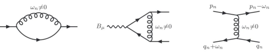
ωn6=0

ωn6=0

Bµ ωn6=0

pn

qn+ωn

pn−ωn

qn

Figure 1. The graphs for determining the effective mass parameter (left), the effective coupling of the vector current to the low-energy modes (middle), as well as 4-quark operators (right).

from eq. (4.8), whereas for V₀⁽⁰⁾ the elimination of non-propagating modes (separately for pn>0 andpn<0) yields

V₀^(0;pn)=χ^†_pnχ_pn+φ^†_pnφ_pn = ǫ_ij 2ip_n

φ^†_pnσ_i←D→_jχ_pn−χ^†_pnσ_i←D→_jφ_pn

+O 1

p²_n

. (4.12) This is clearly a P-channel operator.

5 Mass and vertex corrections

In the discussion of the previous section, only Matsubara zero modes of gauge fields ap- peared. In full QCD, there are obviously also non-zero Matsubara modes. The description of eqs. (4.8), (4.10) should be viewed as a low-energy effective theory from which the non- zero Matsubara modes have been integrated out. The effect of the integration out is to mod- ify the parameters of the low-energy description, and this is the topic of the present section.

Before proceeding, let us discuss the kinematic regime relevant for the problem. As became clear in section3, fork_n6= 0 the long-distance screening concerns a distance scale z ∼ 1/kn and is therefore determined by the kinematic regime K² = k_n² +k₃² ∼ 0. As was discussed in section 4 (cf. e.g. eq. (4.9)), the quark Matsubara modes are close to on-shell, with P² = p²_n+p²₃ ∼ 0. In a typical case (as discussed in more detail below) the two “constituents” have the Matsubara modes pn = kn/2. Therefore, even though we are considering a Euclidean problem, the kinematics is formally similar to that of collinear splitting, in which a nearly on-shell photon with Minkowskian four-momentum K = (k⁰,k) splits into two fermions with four-momenta P =K/2. This formal similarity suggests a relationship of the current problem to that of photon (K² = 0) or soft-dilepton (K² ∼g²T²) production from a QCD plasma.

The similarity turns out to extend into practical computations, notably the de- termination of effects from non-zero Matsubara modes. Indeed, the mass and vertex corrections induced by the non-zero modes can be extracted from computations which are essentially equivalent to the derivation of the Hard Thermal Loop (HTL) effective action [21, 22]. The reason is that the assumptions needed in the computations are K² ≪ (πT)², P² ≪ (πT)²,(K−P)² ≪ (πT)², which as we have argued are true in our situation as well. The graphs to be considered are shown in figure 1, in which a 4-quark operator has been included as well (cf. ref. [20]).

JHEP05(2014)117

After computing the graphs and expanding to leading order in K²/(πT)², P²/(πT)²,(K − P)²/(πT)², the results can be expressed as corrections to the actions in eqs. (4.8), (4.10). Using for the moment the original fermion fields, the free part of S0 becomes²

S₀ =P Z

{P}

iψ(P¯ )

/

P +m²_∞ 2

Z

v

iγ₀+v·γ ip_n+v·p

ψ(P), (5.1)

whereP = (p_n,p), P/ ≡γ_µP_µ,v·γ≡v_iγ_i, and R

v is the integral over directions of a unit vector (|v|= 1), normalized as R

v1 = 1. The “asymptotic mass” parameter reads m²_∞≡ g²T²CF

4 . (5.2)

The coupling to the vector current is S_B =P

Z

{P,R},K

ψ(P¯ )

/

B(K)−m²_∞ 2

Z

v

(iγ₀+v·γ)(iB0+v·B)(K) (ip_n+v·p)(ir_n+v·r)

ψ(R) ¯δ(K−P+R). (5.3) It might be expected that the correction here is suppressed by O(m²_∞/p²_n) ∼ O(α_s), but this is not the case, because parts of the velocity integral give terms ofO(m²_∞/P²)∼ O(1).

Let us define an “on-shell” spinoru satisfying

/

P +m²_∞ 2

Z

v

iγ₀+v·γ ip_n+v·p

u(P) = 0. (5.4)

Consider the dispersion relation following from eq. (5.4). It is known that in Minkowskian space-time the dispersion relation of the “particle branch” readsp⁰ =p+m²_∞/(2p) +. . ., where p = |p| [23]. Continuing the frequency to imaginary time, this corresponds to p²_n+p²₃+p²_⊥ =−m²_∞. Solving for p₃ with a fixedp_nyields

±ip₃ =p_n+ m²_∞ 2p_n + p²_⊥

2p_n +. . . . (5.5)

From here a “rest mass” can be identified and subsequently used as a matching coefficient, M_n≡p_n+ m²_∞

2p_n +O(α²_sT). (5.6)

This agrees with the effective mass derived from an explicit matching computation in ref. [12]; a derivation through HTL expressions like above was previously presented in ref. [24].

The computation of the vertex correction is more cumbersome; however, the task can be simplified by carrying out the matching with the special kinematics³ R =−P =−K/2, in an “on-shell” configuration. Consider the matrix element

Γ(B) ≡ u(P)¯

/

B(K) +m²_∞ 2

Z

v

(iγ₀+v·γ)(iB0+v·B)(K) (ip_n+v·p)²

u(−P), K= 2P . (5.7)

2In this section spatial vectors are three-dimensional and latin indices run from 1 to 3.

3This trick can only be used ifkn/2 is an odd multiple ofπT, however we assume the result to be general.

JHEP05(2014)117

The velocity integrals appearing here are all doable. In particular, it can be shown that the transverse part of the current, i.e. the part coupling to B_T with p_⊥·B_T = 0, has a coefficientO(m²_∞/p²₃)∼ O(α_s); this correction will be neglected in the following.

As far as the longitudinal parts are concerned, we focus on the component coupling to B₀ like before (cf. eq. (2.5)). An explicit computation yields

B₀ Z

v

iγ₀+v·γ

(ip_n+v·p)² =−B₀ P²

iγ₀− ip_np·γ p²

+O 1 p²

. (5.8)

Inserting P²=−m²_∞ and |p_⊥| ≪ |p3| ∼ |pn| we get a correction ofO(1), so that eq. (5.7) becomes

Γ(B₀) =B₀u(P¯ ) 1

2

γ₀+p_n p3

γ₃

u(−P) +O(α_s). (5.9) Rewriting this with 2-component spinors like in eq. (4.8), the HTL-corrected vertex for the operator to whichB₀ couples reads

S_B0 ^pn=k→^n/2 Z

x,z

B₀^(kn)

p₃+ip_n

2p₃ χ^†_pnχ_−pn+p₃−ip_n

2p₃ φ^†_pnφ_−pn

+O(α_s). (5.10) However, for the on-shell configuration ofφ^†pn,p₃ =−ip_n+O(α_s) (cf. eq. (4.7)). Similarly, for on-shell χ^†_pn,p₃ =ip_n+O(α_s). Therefore the prefactors of the operators in eq. (5.10) equal unity. Thus the end result is that for the zero component of the current, we can simply use naive vertices as read off from eq. (4.8).⁴

The non-zero Matsubara modes also induce higher-dimensional operators. In particu- lar, as pointed out in ref. [20], they generate 4-quark operators which can be represented as

δS₀=g²T 2

X

{pn,qn},ωn6=0

1 ω_n²

Z

x,z

χ^†_pnφ^†_pn

γ₀γ_µT^a

χ_pn−ωn φ_pn−ωn

χ^†_qnφ^†_qn

γ₀γ_µT^a

χ_qn+ωn φ_qn+ωn

.

(5.11) Here the matricesγ₀γ_µare as given in eq. (2.7), andT^aare Hermitean generators of SU(3), normalized as Tr [T^aT^b] =δ_ab/2. The role of these operators is that they cause mixings;

for instance, a state ∼φ^†_pn−ωnφ_qn can be transferred to ∼φ^†_pnφ_qn+ωn, both of which have the same screening mass p_n−q_n−ω_n at tree level, but a different “decomposition”. This implies that all decompositions decay with the same screening mass whenδS₀ is included.

6 Schr¨odinger equation

In this section we recall how the computation of the spatial correlators within the effective theory of sections4,5reduces to the solution of a two-dimensional Schr¨odinger equation. In particular, we show that in the free limit eqs. (3.12), (3.13), (3.16), (3.17) can be reproduced this way; and that, going to NLO, the equation to be solved is closely related to that for soft-dilepton and photon production in ref. [11]. The theory is the same as in eq. (4.10), with the modification p_n→M_nas discussed around eq. (5.6).

4It can be shown that in the static sector, kn = 0, all vertex corrections are suppressed byO(αs), so that naive vertices again suffice.

JHEP05(2014)117

6.1 Charge density correlator (G₀₀)

The charge density can be expressed in terms of low-energy fields as (cf. eqs. (4.4), (4.8)) V₀^(kn)= X

0<pn<kn

χ^†_pnχ_pn−kn+φ^†_pnφ_pn−kn

. (6.1)

The fieldsφ^†pn andφ_pn−kn =φ_−|k

n−pn|are forward-propagating and contribute in eq. (4.1) ifz >0. We now rewrite eq. (4.1) with an auxiliary point-splitting in the operator:

G^(k₀₀ⁿ⁾(z) = lim

y,y^′→0T Z

x

D

V₀^(kn)(x, z;y)V₀^(−kn)(0;−y^′)E

c, (6.2)

where (for z >0)

V₀^(kn)(x, z;y) ≡ X

0<pn<kn

φ^†_pn

x+ y 2, z

W_y,zφ_pn−kn

x−y 2 , z

, (6.3)

andW_y,zis a transverse Wilson line. Computing the correlator to leading order in the weak- coupling expansion and taking already the limit y^′ →0, a straightforward analysis yields

G^(k₀₀ⁿ⁾(z) =− X

0<pn<kn

2NcT lim

y→0wLO(z,y) +O(αs), (6.4) where

wLO(z,y)≡ Z

q

e^{−iq·y−(Mcm+ q}

2 2Mr)|z|

. (6.5)

Here

M_cm≡k_n+ m²_∞ 2Mr

, M_r≡ 1

p_n + 1 k_n−p_n

−1

. (6.6)

Two things can be learned from eq. (6.5). First, wLO can equivalently be represented as a solution of a first order differential equation with a particular boundary condition,

∂z+Mcm− ∇² 2Mr

wLO(z,y) = 0, z >0, (6.7) wLO(0,y) = δ⁽²⁾(y). (6.8) Second, the point-split spectral function corresponding to eq. (6.5) can be determined,

ρLO(ω,y) = Z

q

e^−iq·yπδ

ω−M_cm− q² 2Mr

, ω >0. (6.9) The original spectral function thereby becomes, combining eqs. (6.4) and (6.9),

ρ^(k₀₀ⁿ⁾(ω) = − X

0<pn<kn

2N_cT lim

y→0ρLO(ω,y) = − X

0<pn<kn

N_cT M_rθ ω−M_cm

. (6.10) Setting n = 1 and considering the leading order (i.e. m²_∞ → 0), we have M_cm =k₁ and M_r=k₁/4. Then eq. (6.10) agrees with eq. (3.12) when the latter is expanded to leading non-trivial order inω−k1 (the case of generalkn is discussed in appendix A).

JHEP05(2014)117

Consider now NLO corrections to eq. (6.2). Keepingy,y^′ 6=0, the computation can be carried out by omitting the transverse motion suppressed by 1/(2M_r), whereby the quark propagators are straight Wilson lines. Sending z→ ∞and suppressing y^′, we obtain

∂_z+M_cm

wNLO(z,y) ^z→∞= −V_LO⁺(y)wLO(z,y), (6.11) V_LO⁺(y) ≡ g²_ECF

Z

q

1−e^iq·y 1

q² − 1 q²+m²_E

= g_E²CF

2π

lnmEy 2

+γE+K₀(mEy)

, (6.12)

whereC_F = (N_c²−1)/(2N_c);g²_E=g²T is the gauge coupling of the dimensionally reduced theory;m²_E = (^N₃^c+^N₆^f)g²T²is the Debye mass parameter appearing in the static propagator of A0; and K0 is a modified Bessel function.

We finally combine eqs. (6.7), (6.11). If we setwLO ∼ O(1), than according to eq. (6.11), wNLO ∼ O(α_s). Moreover, in the kinematic regime∇ ∼gT of relevance to us, −∇²/M_r∼ O(αs). It follows that, up to a perturbative error of ∼ O(α²_s), we can write

(∂_z+ ˆH⁺)w(z,y) = 0, z >0, (6.13) wherew=wLO+wNLO+. . .and we have denoted

Hˆ⁺ ≡M_cm− ∇² 2Mr

+V⁺. (6.14)

The initial condition remains that same as in eq. (6.8), up to corrections ofO(α_s).

The Schr¨odinger equation and the initial condition can be combined into a single equation by taking a Fourier transform. The system

∂_zw(z,y) =−sign(z) ˆH⁺w(z,y), w(0,y) =δ⁽²⁾(y) (6.15) can formally be solved as w(z,y) = e^−Hˆ+|z|w(0,y). Its Fourier transform (cf. eq. (2.2)) reads

w(k₃,y) =

[ik₃+ ˆH⁺]⁻¹−[ik₃−Hˆ⁺]⁻¹

δ⁽²⁾(y). (6.16) The spectral function follows from the cut. Defining an auxiliary function g(ω,y) as the solution of az-independent inhomogeneous equation

Hˆ⁺−ω−i0⁺

g⁺(ω,y) =δ⁽²⁾(y), (6.17) we obtain (forω >0 and assuming a positive spectrum)

ρ^(k₀₀ⁿ⁾(ω) =− X

0<pn<kn

2NcT lim

y→0Img⁺(ω,y). (6.18) It may be noted that eqs. (6.17), (6.18) bear a close resemblance to the corresponding equations appearing in the LPM resummation of longitudinal modes for dilepton produc- tion, cf. eqs. (22), (24) of ref. [11]. The overall normalizations of g⁺, as determined by the coefficient of the inhomogeneous term, as well as of the parameters appearing do differ, but

JHEP05(2014)117

this is a matter of conventions. In addition some imaginary parts appear differently,⁵ but this is related to the Minkowskian versus Euclidean nature of the observable considered.

The functional form of the potential appearing in ˆH⁺ is identical, as well as the fact that we are looking for a scalar (S-wave) solution, as determined by the inhomogeneous term.

6.2 Transverse current correlator (G_T)

Let us repeat the analysis for the transverse components of the current, cf. eq. (2.6). We again introduce an auxiliary point-splitting into the currents:

G^(k_Tⁿ⁾(z) = lim

y,y^′→0T

2

X

i=1

Z

x

DV_i^(kn)(x, z;y)V_i^(−kn)(0;−y^′)E

c, (6.19)

where, following eq. (4.11), V_i^(kn)(x, z;y)≡ X

0<pn<kn

(6.20)

φ^†_pn

x+y 2 , z

1

p_n− 1 k_n−p_n

←D→_i 4i −

1

p_n+ 1 k_n−p_n

σ₃ǫ_ij←D→_j 4

φ_pn−kn

x−y

2 , z

,

with the notation ←→

Dj ≡W_y,z−→ Dj −←−

DjW_y,z. At leading order, G^(k_Tⁿ⁾(z) =− X

0<pn<kn

N_cT 1

p²_n + 1 (k_n−p_n)²

y→0lim∇ ·vLO(z,y) +O(α_s), (6.21) where we already tooky^′→0 and defined

vLO(z,y)≡ Z

q

iqe^{−iq·y−(Mcm+ q}

2

2Mr)|z|. (6.22)

Like with the charge density, the LO solution can be represented as a differential equation,

∂_z+M_cm− ∇² 2Mr

vLO(z,y) = 0, z >0, (6.23) vLO(0,y) = −∇δ⁽²⁾(y). (6.24) Also, a point-split spectral function corresponding to eq. (6.22) can be determined,

ρLO(ω,y) = Z

q

iqe^−iq·yπδ

ω−M_cm− q² 2Mr

, ω >0. (6.25) The original spectral function thereby becomes (cf. eq. (6.21))

ρ^(k_T,ⁿ_LO⁾(ω) = − X

0<pn<kn

NcT 1

p²_n + 1 (k_n−p_n)²

y→0lim∇ ·ρ_LO(ω,y)

=− X

0<pn<kn

N_cT 1

p²_n + 1 (kn−pn)²

M_r² ω−M_cm

θ ω−M_cm

. (6.26)

5In particular, in LPM resummation the potential plays the role of a “width”.