Research Collection
Doctoral Thesis
High-dimensional Stochastic Approximation: Algorithms and Convergence Rates
Author(s):
Welti, Timo Publication Date:
2020
Permanent Link:
https://doi.org/10.3929/ethz-b-000457220
Rights / License:
In Copyright - Non-Commercial Use Permitted
This page was generated automatically upon download from the ETH Zurich Research Collection. For more information please consult the Terms of use.
High-dimensional Stochastic Approximation: Algorithms
and Convergence Rates
A thesis submitted to attain the degree of DOCTOR OF SCIENCES of ETH ZÜRICH
(Dr. sc. ETH Zürich)
presented by TIMO WELTI
MSc ETH Mathematics, ETH Zürich born on October 1, 1993
citizen of Küsnacht ZH
accepted on the recommendation of
Prof. Dr. Arnulf Jentzen, University of Münster, examiner Prof. Dr. Philipp Grohs, University of Vienna, co-examiner Prof. Dr. Peter Kloeden, Goethe University Frankfurt, co-examiner
Prof. Dr. Siddhartha Mishra, ETH Zürich, co-examiner
2020
Prof. Dr. Philipp Grohs, University of Vienna, co-examiner
Prof. Dr. Peter Kloeden, Goethe University Frankfurt, co-examiner Prof. Dr. Siddhartha Mishra, ETH Zürich, co-examiner
Timo Welti: High-dimensional Stochastic Approximation:
Algorithms and Convergence Rates, ©2020 ETH Diss. No. 26805
Funding: ETH Research Grant ETH-47 15-2
Swiss National Science Foundation Project No. 184220
In virtually any scenario where there is a desire to make quantitative or qualitative pre- dictions, mathematical models are of crucial importance for predicting quantities of in- terest. Unfortunately, many models are based on mathematical objects that cannot be calculated exactly. As a consequence, numerical approximation algorithms that approx- imate such objects are indispensable in practice. These algorithms are often stochastic in nature, which means that there is some form of randomness involved when running them. In this thesis we consider four possibly high-dimensional approximation problems and corresponding stochastic numerical approximation algorithms. More specifically, we prove essentially sharp rates of convergence in the probabilistically weak sense for spatial spectral Galerkin approximations of semi-linear stochastic wave equations driven by mul- tiplicative noise. In addition, we develop an abstract framework that allows us to view full-history recursive multilevel Picard approximation methods from a new perspective and to work out more clearly how these stochastic methods beat the curse of dimen- sionality in the numerical approximation of semi-linear heat equations. Furthermore, we tackle high-dimensional optimal stopping problems by proposing a stochastic numerical approximation algorithm that is based on deep learning. And finally, we study conver- gence in the probabilistically strong sense of the overall error arising in deep learning based empirical risk minimisation, one of the main pillars of supervised learning.
In geradezu jeder Situation, in der quantitative oder qualitative Prognosen gefragt sind, sind mathematische Modelle von enormer Wichtigkeit, um relevante Grössen vorauszu- berechnen. Unglücklicherweise beruhen viele Modelle auf mathematischen Objekten, die nicht exakt berechenbar sind. Folglich sind numerische Näherungsverfahren, die solche Objekte approximieren, in der Praxis unabdingbar. Oft sind diese Verfahren stochasti- scher Natur, was bedeutet, dass eine Art von Zufälligkeit bei ihrer Ausführung involviert ist. In vorliegender Dissertation betrachten wir vier möglicherweise hochdimensionale Nä- herungsprobleme und zugehörige stochastische numerische Näherungsverfahren. Genauer gesagt beweisen wir Raten der Konvergenz im probabilistisch schwachen Sinne, die im We- sentlichen scharf sind, für räumliche spektrale Galerkinapproximationen von semilinearen stochastischen Wellengleichungen, die von multiplikativem Rauschen angetrieben werden.
Ausserdem entwickeln wir einen abstrakten Formalismus, der uns erlaubt, vollhistorisch rekursive Multilevel-Picard-Approximationsverfahren aus einem neuen Blickwinkel zu be- trachten und klarer herauszuarbeiten, wie diese stochastischen Verfahren den Fluch der Dimensionalität in der numerischen Approximation von semilinearen Wärmeleitungsglei- chungen überwinden. Des Weiteren gehen wir hochdimensionale optimale Stoppprobleme an, indem wir ein stochastisches numerisches Näherungsverfahren einführen, das auf Deep Learning beruht. Und schliesslich untersuchen wir Konvergenz im probabilistisch starken Sinne des Gesamtfehlers, der bei Deep-Learning-basierter empirischer Risikominimierung entsteht, einem der zentralen Standbeine des überwachten Lernens.
The present thesis is a cumulative dissertation. More precisely, Section1.1combined with Chapter 2 is a slightly modified version of the preprint Jacobe de Naurois, Jentzen, &
Welti [185], Section 1.2 combined with Chapter 3 is a slightly modified version of the preprint Giles, Jentzen, & Welti [134], Section 1.3 combined with Chapter 4 is a slightly modified version of the preprint Becker, Cheridito, Jentzen, & Welti [30], and parts of two paragraphs in the beginning of Chapter 1 combined with Section 1.4 and Chapter 5 are a slightly modified version of the preprint Jentzen & Welti [196].
In the case of each of the preprints [134, 185, 196] I have made major contributions in all aspects of the creation of the work, that is, in the development of the ideas in the work, in the development of the proofs in the work, and in the writing of the work. In the case of the preprint [30] I have made major contributions in the development of the proofs in the work, in the development of the computational examples in the work, in the development of the Matlab source codes in the work, and in the writing of the work.
First and foremost I express my deep gratitude to my doctoral advisor Arnulf Jentzen for offering me the chance to do this PhD, for teaching me invaluable lessons about the nature of mathematics, for having countless exciting and inspiring research discussions with me, and for being a constant source of great encouragement and support. I consider myself extremely lucky to have had both the freedom to work independently whenever I wanted to and an advisor who would spare time for me as soon as I had any item to discuss.
I also owe very special thanks to Philipp Grohs, who welcomed me for a research stay at the University of Vienna, and to Mike Giles, who welcomed me for a research stay at the University of Oxford. I thank them for very enriching research discussions and for creating such a friendly atmosphere that allowed me to enjoy my research stays to the fullest. In addition, many thanks are due to my other co-authors Diyora Salimova, Sebastian Becker, Patrick Cheridito, Sonja Cox, Martin Hutzenthaler, Jan van Neerven, Adam Andersson, Ryan Kurniawan, and Ladislas Jacobe de Naurois for very pleasant and productive collaborations. In addition, I am indebted to my co-examiners Philipp Grohs, Peter Kloeden, and Siddhartha Mishra for their readiness to review this thesis and their valuable support.
Financial support through the ETH Research Grant ETH-47 15-2 Mild stochastic cal- culus and numerical approximations for nonlinear stochastic evolution equations with Lévy noise, through the project Deep artificial neural network approximations for stochastic partial differential equations: Algorithms and convergence proofs (project number 184220) funded by the Swiss National Science Foundation, and through the project Construction of New Smoothness Spaces on Domains (project number I 3403) funded by the Austrian Science Fund is gratefully acknowledged. Moreover, I gratefully acknowledge financial support from the Zurich Graduate School in Mathematics.
My time at the SAM has been a truly enjoyable one, for which I thank all current and former SAMmies very much. I especially thank Adrian Ruf, Alice Vanel, Bryn Davies, Carlo Marcati, Carlos Parés Pulido, Diyora Salimova, Fabian Müller, Gina Magnussen, Jakob Zech, Kjetil Olsen Lye, Larisa Yaroslavtseva, Luc Grosheintz Laval, Lukas Herr- mann, Maxim Rakhuba, Michaela Szölgyenyi, Pancho Romero, Philippe von Wurstem- berger, Pratyuksh Bansal, Primož Pušnik, Soumil Gurjar, and Tandri Gauksson for all the laughs, discussions, lunches, and good memories. In addition, I am grateful to David Rottensteiner, Dennis Elbrächter, Julius Berner, Martin Rathmair, Pavol Harár, Rafael Reisenhofer, Sarah Koppensteiner, and Thomas Peter for so kindly welcoming me as one of their peers at the University of Vienna. I am also indebted to Alberto Paganini, Carolina Urzúa Torres, Jaroslav Fowkes, Priya Subramanian, and Yuji Nakatsukasa for making my working environment at the University of Oxford such a pleasant one.
Suter, and Seraina Hügli for their constant support and for these great conversations. I thank my long-distance friends Philipp Dufter, Cynthia Ho, and Leo Wossnig for being close and for letting also the physical distance occasionally be short. I thank Sophie Beck, Jelena Hess, Mauro Hermann, Onur Sazpinar, Carmen Weber, Dominique Eichenberger, Elena Steinrisser, Jakob Herzog, Maria Engel, Rafael Hug, Jana Huisman, Nicole Speck, Beda Büchel, Lukas Ryffel, Philippe Degen, and Robert Knell for making me laugh, for lending an ear, for giving words of advice, and for keeping in touch. I thank Frederik Benzing and Alexis Podolak for being fantastic flatmates. I thank Christopher Gordon and Ludwig Hruza for playing with me in the string trio des amis. I thank Franzi Schiegl, Freede Metje, Anna Siegert, Cinzia Zanovello, Laura Kömürcü, Marlene Baumgartner, and Sebastian Maurer for making my time in Vienna unforgettable. I thank Anja Bitter- wolf, Constanze Cavalier, Maike Ludley, Mario Hörbe, and Sara Schöchli for making me feel at home in Oxford.
I would not have been able to achieve anything without the life-long support from my parents Renate Salzgeber and Martin Welti and my sister Nora Welti. I thank them for everything, for their counsel, for cutting me some slack.
Finally, with all my heart I thank Andrea Gollner for her love, for always being there for me, for being awesome. You are the best thing that has ever happened to me.
Timo Welti Zürich, April 2020
Abstract iii
Zusammenfassung v
Preface vii
Acknowledgements ix
1 Introduction 1
1.1 Stochastic wave equations . . . 3
1.2 Generalised multilevel Picard approximations . . . 6
1.3 Optimal stopping problems . . . 10
1.4 Empirical risk minimisation . . . 12
2 Stochastic wave equations 17 2.1 Preliminary results . . . 17
2.1.1 Notation . . . 18
2.1.2 Well-posedness and regularity of stochastic evolution equations . . . 19
2.1.3 Setting . . . 22
2.1.4 Basic properties of deterministic linear wave equations . . . 23
2.2 Upper bounds for weak errors . . . 25
2.2.1 Setting . . . 26
2.2.2 Weak convergence rates for Galerkin approximations . . . 26
2.2.3 Semi-linear stochastic wave equations . . . 36
3 Generalised multilevel Picard approximations 45 3.1 Generalised full-history recursive multilevel Picard (MLP) approximations 46 3.1.1 Measurability involving the strong σ-algebra . . . 47
3.1.2 Identities involving bias and variance in Hilbert spaces . . . 48
3.1.2.1 Bias–variance decomposition . . . 48
3.1.2.2 Generalised bias–variance decomposition . . . 48
3.1.2.3 Variance identity . . . 49
3.1.2.4 Generalised variance identity . . . 50
3.1.3 Properties of generalised MLP approximations . . . 51
3.1.4 Error analysis . . . 53
3.1.5 Cost analysis . . . 59
3.1.6 Complexity analysis . . . 61
3.2 MLP for semi-linear heat equations . . . 66
3.2.1.2 Sufficient conditions for strictly slower growth . . . 70
3.2.1.3 Growth estimate for compositions . . . 71
3.2.2 Verification of the assumed properties . . . 72
3.2.2.1 Setting . . . 72
3.2.2.2 Measurability . . . 73
3.2.2.3 Recursive formulation . . . 78
3.2.2.4 Integrability . . . 79
3.2.2.5 Estimates . . . 82
3.2.3 Complexity analysis . . . 88
3.2.3.1 MLP approximations in fixed space dimensions . . . 88
3.2.3.2 MLP approximations in variable space dimensions . . . 91
4 Optimal stopping problems 95 4.1 Main ideas of the proposed algorithm . . . 96
4.1.1 The American option pricing problem . . . 96
4.1.2 Temporal discretisation . . . 97
4.1.3 Factorisation lemma for stopping times . . . 98
4.1.4 Neural network architectures for stopping times . . . 100
4.1.5 Formulation of the objective function . . . 102
4.1.6 Stochastic gradient ascent optimisation algorithms . . . 103
4.1.7 Price and optimal exercise time for American-style options . . . 103
4.2 Details of the proposed algorithm . . . 104
4.2.1 Formulation of the proposed algorithm in a special case . . . 104
4.2.2 Formulation of the proposed algorithm in the general case . . . 106
4.2.3 Comments on the proposed algorithm . . . 107
4.3 Numerical examples of pricing American-style derivatives . . . 108
4.3.1 Theoretical considerations . . . 109
4.3.2 Setting . . . 112
4.3.3 Examples with known one-dimensional representation . . . 114
4.3.3.1 Optimal stopping of a Brownian motion . . . 114
4.3.3.2 Geometric average-type options . . . 115
4.3.4 Examples without known one-dimensional representation . . . 120
4.3.4.1 Max-call options . . . 120
4.3.4.2 A strangle spread basket option . . . 125
4.3.4.3 A put basket option in Dupire’s local volatility model . . . 126
4.3.4.4 A path-dependent financial derivative . . . 128
5 Empirical risk minimisation 131 5.1 Basics on deep neural networks (DNNs) . . . 132
5.1.1 Vectorised description of DNNs . . . 132
5.1.2 Activation functions . . . 132
5.1.3 Rectified DNNs . . . 133
5.2 Analysis of the approximation error . . . 133
5.2.1 A covering number estimate . . . 134
5.2.2 Convergence rates for the approximation error . . . 135
5.3.2 Uniform strong error estimates for random fields . . . 140
5.3.3 Strong convergence rates for the generalisation error . . . 144
5.4 Analysis of the optimisation error . . . 149
5.4.1 Properties of the gamma and the beta function . . . 150
5.4.2 Strong convergence rates for the optimisation error . . . 153
5.5 Analysis of the overall error . . . 158
5.5.1 Overall error decomposition . . . 159
5.5.2 Overall strong error analysis for the training of DNNs . . . 160
5.5.3 Stochastic gradient descent with random initialisation . . . 168
6 Conclusion and Outlook 171 6.1 Stochastic wave equations . . . 171
6.2 Generalised multilevel Picard approximations . . . 172
6.3 Optimal stopping problems . . . 173
6.4 Empirical risk minimisation . . . 174
References 177
Curriculum vitae
Chapter 1
Introduction
Mathematical modelling is ubiquitous. In virtually any scenario where there is a desire to make quantitative or qualitative predictions, theoretical insights and gathered data are used to derive mathematical models with the aim to predict values of quantities of interest. To name but a few examples, mathematical models for randomness allow us to make predictions based on statistics, mathematical models for the lift force enable us to construct wings that carry a modern airplane, mathematical models from quantum mechanics pave the way for the design and study of quantum computers, mathematical models that find a majority in parliament and the electorate tell us how much taxes we are obligated to pay, and mathematical models for infectious diseases provide us with possible scenarios for the evolution of a pandemic. In many cases reaching an actual prediction from the derived mathematical model requires solving equations or computing numbers that are not given in an explicit way. Unfortunately, this cannot be done exactly for the vast majority of mathematical models of practical relevance. For this reason, numerical approximation algorithms which are capable of approximatively solving certain equations or approximatively computing certain numbers are required.
Often such numerical approximation algorithms are stochastic in nature, which means that there is some form of randomness involved when running them. On the one hand, this randomness may stem directly from the mathematical model, which may incorporate randomness itself in order to achieve more realistic predictions. This is, for example, the case when numerically approximating solutions of stochastic partial differential equations (SPDEs), when numerically solving optimal stopping problems, and when using machine learning algorithms in order to approximatively solve supervised learning problems. On the other hand, randomness in numerical approximation algorithms may be beneficial even though the mathematical model under consideration is purely deterministic. Ex- amples for this situation include Monte Carlo methods for approximatively computing high-dimensional deterministic integrals or stochastic numerical approximation methods for solving deterministic partial differential equations (deterministic PDEs). In this the- sis we consider four possibly high-dimensional approximation problems and corresponding stochastic numerical approximation algorithms.
We first analyse spatial spectral Galerkin approximations of a certain class of semi- linear stochastic wave equations (cf. Section 1.1 and Chapter2). In order to develop our analysis for the approximation error and to prove essentially sharp convergence rates, we interpret solutions of the considered stochastic wave equations as solutions of suitable
infinite-dimensional stochastic evolution equations. In this sense the problem of numeri- cally approximating semi-linear stochastic wave equations is extremely high-dimensional.
Thereafter, we examine full-history recursive multilevel Picard (MLP) approximation methods (cf. E et al. [111] and Hutzenthaler et al. [181]), which are stochastic numer- ical approximation methods capable of solving high-dimensional PDEs (cf. Section 1.2 and Chapter 3). We establish an abstract framework for suitably generalised MLP ap- proximation methods which take values in possibly infinite-dimensional Banach spaces and use this framework to prove a computational complexity result for suitable MLP approximation methods for semi-linear heat equations. This computational complexity result illustrates, in particular, how the overall computational cost grows with the space dimension of the approximated semi-linear heat equation.
In connection with the third and fourth numerical approximation problems, we con- sider stochastic numerical approximation algorithms that are based on deep learning.1 Deep learning based algorithms have been applied extremely successfully to overcome fundamental challenges in many different areas, such as image recognition, natural lan- guage processing, game intelligence, autonomous driving, and computational advertising, just to name a few. Accordingly, researchers from a wide range of different fields, includ- ing, for example, computer science, mathematics, chemistry, medicine, and finance, are investing significant efforts into studying such algorithms and employing them to tackle challenges arising in their fields. In this spirit we propose a deep learning based stochastic numerical approximation algorithm for solving possibly high-dimensional optimal stop- ping problems (cf. Section1.3 and Chapter4). We provide evidence for the effectiveness and efficiency of the proposed algorithm in the case of high-dimensional optimal stop- ping problems by presenting results for many numerical example problems with different numbers of dimensions.
In spite of the, as mentioned, broad research interest and the accomplishments of deep learning based algorithms in numerous applications, at the moment there is still no rig- orous understanding of the reasons why such algorithms produce useful results in certain situations.2 Consequently, there is no rigorous way to predict, before actually implement- ing a deep learning based algorithm, in which situations it might perform reliably and in which situations it might fail. This necessitates in many cases a trial-and-error approach in order to move forward, which can cost a lot of time and resources. A thorough math- ematical analysis of deep learning based algorithms (in scenarios where it is possible to formulate such an analysis) seems to be crucial in order to make progress on these issues.
Moreover, such an analysis may lead to new insights that enable the design of more ef- fective and efficient algorithms. With this situation in mind, we investigate deep learning based empirical risk minimisation, a stochastic numerical approximation algorithm that is one of the main pillars of supervised learning (cf. Section 1.4 and Chapter 5). More specifically, we prove mathematically rigorous convergence results for the overall error by deriving convergence rates for the three different sources of error, that is, for the approx- imation error, the generalisation error, and the optimisation error. These convergence results are applicable without any restriction on the number of dimensions of the domain on which the function to be learned is defined.
In the following we explain our work on these four numerical approximation problems and the corresponding stochastic numerical approximation algorithms in more detail.
1Parts of this paragraph are a slightly modified extract of the preprint Jentzen & Welti [196].
2Parts of this paragraph are a slightly modified extract of the preprint Jentzen & Welti [196].
1.1 Stochastic wave equations
In the field of numerical approximation of stochastic evolution equations one distinguishes between two conceptually fundamentally different error criteria, that is, strong conver- gence and weak convergence. In the case of the finite-dimensional stochastic ordinary differential equations, both strong and weak convergence are quite well understood nowa- days; cf., e.g., the standard monographs Kloeden & Platen [203] and Milstein [246]. How- ever, the situation is different in the case of the infinite-dimensional SPDEs (cf., e.g., Walsh [299], Da Prato & Zabczyk [94], Liu & Röckner [230]). In the case of SPDEs with regular non-linearities, strong convergence rates are essentially well understood, whereas a proper understanding of weak convergence rates has still not been reached (cf., e.g., [7, 8, 54–56, 82, 86, 98–100, 132, 162, 165, 166, 185, 191, 210–212, 214, 215, 228, 283, 302–304] for several weak convergence results in the literature). In Chapter 2 and the preprint Jacobe de Naurois, Jentzen, & Welti [185], of which the current section com- bined with Chapter2 is a slightly modified version, we derive weak convergence rates for stochastic wave equations. Stochastic wave equations can be used for modelling several evolutionary processes subject to random forces. Examples include the motion of a DNA molecule floating in a fluid and the dilatation of shock waves throughout the sun (cf., e.g., Dalang [95, Section 1]) as well as heat conduction around a ring (cf., e.g., Thomas [292]).
Unfortunately, such problems usually involve complicated non-linearities and are inac- cessible for current numerical analysis approaches. Nonetheless, rigorous examination of simpler model problems such as the ones considered in Chapter 2 and the preprint [185], respectively, is a key first step. Even though a number of strong convergence rates for stochastic wave equations are available (cf., e.g., [9,79,80,213,265,300,302,305]), apart from the findings of the preprint [185] and of the subsequent works Harms & Müller [162]
and Cox, Jentzen, & Lindner [86] the existing weak convergence results for stochastic wave equations in the literature (cf., e.g., [166, 211, 212, 214, 302, 303]) assume that the diffusion coefficient is constant or, in other words, that the equation is driven by additive noise.
The main contribution of Chapter 2and the preprint [185], respectively, is the deriva- tion of essentially sharp weak convergence rates for a class of stochastic wave equations large enough to also include the case of multiplicative noise. Roughly speaking, the main result of Chapter 2 (cf. Theorem 2.12 in Subsection 2.2.2) and of the preprint [185] (cf.
[185, Theorem 3.7]), respectively, establishes upper bounds for weak errors associated to spatial spectral Galerkin approximations of semi-linear stochastic wave equations under suitable Lipschitz and smoothness assumptions on the drift non-linearity and on the dif- fusion coefficient as well as under suitable integrability and regularity assumptions on the initial value. In order to employ a mild solution framework, the second-order stochas- tic wave equations are formulated as first-order two-component systems of stochastic evolution equations on an extended state space. The first component process of the solution process of such a first-order system corresponds to the solution process of the original second-order equation, while the second component process corresponds to the time derivative of the first component process. As is often the case in the context of spa- tial spectral Galerkin approximations, convergence is obtained in terms of the in absolute value increasing sequence of eigenvalues of a symmetric linear operator.
To illustrate the main result of Chapter 2 and the preprint [185], respectively, in more detail, we consider the following setting as a special case of our general framework (cf. Subsection 2.2.1). Consider the notation in Subsection 2.1.1, let (H,h·,·iH,k·kH)
and (U,h·,·iU,k·kU) be separable R-Hilbert spaces, let T ∈ (0,∞), let (Ω,F,P) be a probability space with a normal filtration (Ft)t∈[0,T], let (Wt)t∈[0,T] be an idU-cylindrical (Ω,F,P,(Ft)t∈[0,T])-Wiener process, let (en)n∈N={1,2,3,...} ⊆ H be an orthonormal basis of H, let (λn)n∈N ⊆ (0,∞) be an increasing sequence, let A: D(A) ⊆ H → H be the linear operator which satisfies D(A) =
v ∈ H: P∞
n=1|λnhen, viH|2 < ∞ and ∀v ∈ D(A) :Av =P∞
n=1−λnhen, viHen, let(Hr,h·,·iHr,k·kHr), r∈R, be a family of interpola- tion spaces associated to−A (cf., e.g., [279, Section 3.7]), let (Hr,h·,·iHr,k·kHr), r ∈R, be the family ofR-Hilbert spaces which satisfies for all r ∈R that (Hr,h·,·iHr,k·kHr) =
Hr/2 × Hr/2−1/2,h·,·iHr/2×Hr/2−1/2,k·kHr/2×Hr/2−1/2
, let PN ∈ L(H0), N ∈ N ∪ {∞}, be the linear operators which satisfy for all N ∈ N ∪ {∞}, v, w ∈ H that PN(v, w) =
PN
n=1hen, viHen,PN
n=1hen, wiHen
, let A: D(A) ⊆ H0 → H0 be the linear operator which satisfies D(A) = H1 and ∀(v, w) ∈ H1: A(v, w) = (w, Av), and let γ ∈ (0,∞), β∈(γ/2, γ], ρ∈[0,2(γ−β)],%, CF, CB ∈[0,∞),ξ ∈L2(P|F0;H2(γ−β)),F∈Lip0(H0,H0), B∈ Lip0(H0, L2(U,H0)) satisfy (−A)−β ∈ L1(H), F(Hρ) ⊆H2(γ−β), (Hρ 3 v 7→ F(v)∈ H2(γ−β)) ∈ Lip0(Hρ,H2(γ−β)), ∀v ∈ Hρ, u ∈ U: B(v)u ∈ Hγ, ∀v ∈ Hρ: (U 3 u 7→
B(v)u ∈ Hρ) ∈ L2(U,Hρ), (Hρ 3 v 7→ (U 3 u 7→ B(v)u ∈ Hρ) ∈ L2(U,Hρ)) ∈ Lip0(Hρ, L2(U,Hρ)), ∀v ∈ Hρ: (U 3 u 7→ B(v)u ∈ Hγ) ∈ L(U,Hγ), (Hρ 3 v 7→ (U 3 u 7→ B(v)u ∈ Hγ) ∈ L(U,Hγ)) ∈ Lip0(Hρ, L(U,Hγ)), F|H% ∈ C2(H%,H0), B|H% ∈ C2(H%, L2(U,H0)), CF = supx,v1,v2∈∩r∈
RHr,max{kv1kH0,kv2kH0}≤1kF00(x)(v1, v2)kH0 <∞, and CB = supx,v1,v2∈∩r∈
RHr,max{kv1kH0,kv2kH0}≤1kB00(x)(v1, v2)kL2(U,H0) <∞. Theorem 1.1. Assume the above setting. Then
(i) it holds that there exist up to modifications unique (Ft)t∈[0,T]-predictable stochastic processes XN = (XN,XN) : [0, T]×Ω→ PN(Hρ), N ∈ N∪ {∞}, such that for all N ∈N∪ {∞}, t∈[0, T] it holds that sups∈[0,T]E
kXNs k2Hρ
<∞ and P-a.s. that XNt =etAPNξ+
Z t 0
e(t−s)APNF(XNs ) ds+ Z t
0
e(t−s)APNB(XNs ) dWs (1.1) and
(ii) it holds that sup
N∈N
sup
ϕ∈Cb2(H0,R)\{0}
(λN)γ−β E
ϕ X∞T
−E
ϕ XNT kϕkC2
b(H0,R)
≤max 1,E
kξk2H
ρ
h E
kξkH2(γ−β) +T
F|Hρ
Lip0(Hρ,H2(γ−β))
+ 2Tk(−A)−βkL1(H) B|Hρ
2
Lip0(Hρ,L(U,Hγ))
i maxn
1,
T (CF)2+ 2 (CB)21/2o
·exp T1
2 + 3|F|Lip0(H0,H0)+ 4|B|2Lip0(H0,L2(U,H0))
(1.2)
·exp Th
2 F|Hρ
Lip0(Hρ,Hρ)+ B|Hρ
2
Lip0(Hρ,L2(U,Hρ))
i
<∞.
Theorem1.1 follows directly from Remark2.7 and Corollary 2.14in Subsection2.2.2, the latter of which is a consequence of Theorem 2.12 in Subsection 2.2.2. Let us now add a few remarks regarding Theorem1.1.
First, we briefly outline our proof of Theorem 1.1. As usual in the case of weak convergence analysis, the Kolmogorov equation (cf. (2.58) in the proof of Theorem 2.12) is used. Another key ingredient is the Hölder inequality for Schatten norms (cf. (2.61) in
the proof of Theorem 2.12). In addition, the proof of Theorem 1.1 employs the mild Itô formula (cf. Da Prato, Jentzen, & Röckner [93, Corollary 1]) to obtain suitable a priori estimates for solutions of (1.1) above (cf. Lemma 2.8in Subsection2.2.2 for details). The detailed proof of Theorems 1.1 and 2.12, respectively, can be found in Subsection2.2.2.
Second, we would like to emphasise that in the general setting of Theorem 1.1, the weak convergence rate established in Theorem 1.1 can essentially not be improved. More precisely, Jacobe de Naurois, Jentzen, & Welti [186, Theorem 1.1] proves that for every η∈(0,∞)and every infinite-dimensional separableR-Hilbert space(H,h·,·iH,k·kH)there exist(U,h·,·iU,k·kU),A: D(A)⊆H →H,γ, c∈(0,∞), (Cε)ε∈(0,∞) ⊆[0,∞), ρ∈[0,γ/2], ξ ∈ L2(P|F0;Hγ), ϕ ∈ Cb2(H0,R), F ∈ Cb2(H0,H0), B ∈ Cb2(H0, L2(U,H0)) such that F(Hρ) ⊆ Hγ, (Hρ 3 v 7→ F(v) ∈ Hγ) ∈ Lip0(Hρ,Hγ), ∀v ∈ Hρ, u ∈ U: B(v)u ∈ Hγ,
∀v ∈ Hρ: (U 3 u 7→ B(v)u ∈ Hρ) ∈ L2(U,Hρ), (Hρ 3 v 7→ (U 3 u 7→ B(v)u ∈ Hρ) ∈ L2(U,Hρ)) ∈ Lip0(Hρ, L2(U,Hρ)), ∀v ∈ Hρ: (U 3 u 7→ B(v)u ∈ Hγ) ∈ L(U,Hγ), and (Hρ3 v 7→(U 3u7→ B(v)u∈Hγ)∈ L(U,Hγ))∈Lip0(Hρ, L(U,Hγ)) and such that for allε ∈(0,∞), N ∈N it holds that
c·(λN)−η ≤ E
ϕ X∞T
−E
ϕ XNT
≤Cε·(λN)ε−η. (1.3) Further results on lower bounds for strong and weak errors for stochastic parabolic equa- tions can be found, e.g., in Davie & Gaines [96], Müller-Gronbach, Ritter, & Wagner [251], Müller-Gronbach & Ritter [250], Conus, Jentzen, & Kurniawan [82], and Jentzen & Kur- niawan [191].
Third, we illustrate Theorem 1.1 by a simple example (cf. Corollary 2.18 in Sub- section 2.2.3). For this let PN ∈ L(H), N ∈ N∪ {∞}, be the linear operators which satisfy for all N ∈ N ∪ {∞}, v ∈ H that PN(v) = PN
n=1hen, viHen. In the case where (H,h·,·iH,k·kH) = (U,h·,·iU,k·kU) = L2(µ(0,1);R),h·,·iL2(µ(0,1);R),k·kL2(µ(0,1);R)
, ξ = (ξ0, ξ1)∈ H01((0,1);R)×H, and F = 0, where A: D(A) ⊆H →H is the Laplacian with Dirichlet boundary conditions on H, and where B: H×H−1/2 →L2(H, H ×H−1/2) is the function which satisfies for all (v, w) ∈ H×H−1/2, u ∈ C([0,1],R) and µ(0,1)-a.e.
x∈(0,1)that B(v, w)u
(x) = 0, v(x)u(x)
, the first component processesXN: [0, T]× Ω→PN(H),N ∈N∪ {∞}, are mild solutions of the SPDEs
X¨t(x) = ∂x∂22Xt(x) +PNXt(x) ˙Wt(x) (1.4) with X0(x) = (PNξ0)(x), X˙0(x) = (PNξ1)(x), and Xt(0) = Xt(1) = 0 for x ∈ (0,1), t∈[0, T], N ∈N∪ {∞}. In the caseN =∞, (1.4) is known as the continuous version of the hyperbolic Anderson model in the literature (cf., e.g., Conus et al. [83]). Theorem 1.1 applied to (1.4) ensures for allϕ∈ Cb2(H,R), ε ∈(0,∞) that there exists a real number C ∈[0,∞) such that for all N ∈Nit holds that
E
ϕ XT∞
−E
ϕ XTN
≤C·Nε−1 (1.5)
(cf. Corollary 2.18). We thus prove that the spatial spectral Galerkin approximations converge with weak rate 1- to the solution of the continuous version of the hyperbolic Anderson model. The weak rate 1- is exactly twice the well-known strong convergence rate for the continuous version of the hyperbolic Anderson model. To the best of our knowledge, Theorem 1.1 and the corresponding result [185, Theorem 1.1], respectively, are the first result in the literature that establishes an essentially sharp weak convergence rate for the continuous version of the hyperbolic Anderson model. Theorem 1.1 also establishes essentially sharp weak convergence rates for more general semi-linear stochastic wave equations (cf. Corollaries 2.16 and 2.18 in Subsection 2.2.3).
1.2 Generalised multilevel Picard approximations
It is one of the most challenging problems in applied mathematics to approximatively solve high-dimensional PDEs. In particular, most of the numerical approximation schemes studied in the scientific literature, such as finite differences, finite elements, and sparse grids, suffer under the curse of dimensionality (cf. Bellman [32]) in the sense that the number of computational operations needed to compute an approximation with an error of size at most ε > 0 grows at least exponentially in the PDE dimension d ∈ N or in the reciprocal of ε. Computing such an approximation with reasonably small error thus becomes unfeasible in dimension greater than, say, ten. Therefore, a fundamental goal of current research activities is to propose and analyse numerical methods with the power to beat the curse of dimensionality in such way that the number of computational oper- ations needed to compute an approximation with an error of size at most ε >0 grows at most polynomially in both the PDE dimension d ∈ N and the reciprocal of ε (cf., e.g., Novak & Woźniakowski [253, Chapter 1; 254, Chapter 9]). In the recent years a number of numerical schemes have been proposed to tackle the problem of approximately solving high-dimensional PDEs, which include deep learning based approximation methods (cf., e.g., [21–23, 28, 30, 45, 66, 75, 106, 110, 117, 123, 127, 146, 158, 159, 169, 178, 187, 231, 234, 238, 262, 266, 288] and the references mentioned therein), branching diffusion approximation methods (cf., e.g., [1, 31, 46, 51, 52, 67,168, 170–172, 241, 267,289, 306, 307]), approximation methods based on discretising a corresponding backward stochas- tic differential equation (BSDE) using iterative regression on function Hamel bases (cf., e.g., [13, 40, 43, 53, 68–71, 87–90, 101, 107, 137–142, 177, 219, 225, 229, 235–237, 247, 248,261,272–274, 296,312] and the references mentioned therein) or using Wiener chaos expansions (cf. Briand & Labart [57] and Geiss & Labart [131]), and MLP approximation methods (cf. [25, 26, 111, 112, 134, 179, 181–183]). So far, deep learning based approxi- mation methods for PDEs seem to work very well in the case of high-dimensional PDEs judging from a large number of numerical experiments. However, there exist only partial results (cf., e.g., [47, 120, 144, 148–150, 180, 194, 218, 268]) and no full error analysis in the scientific literature rigorously justifying their effectiveness in the numerical approxi- mation of high-dimensional PDEs. Moreover, while for branching diffusion methods there is a full error analysis available proving that the curse of dimensionality can be beaten for instances of PDEs with small time horizon and small initial condition, respectively, numerical simulations suggest that such methods fail to work if the time horizon or the initial condition, respectively, are not small anymore. To sum it up, MLP approximation methods currently are, to the best of our knowledge, the only methods for parabolic semi- linear PDEs with general time horizons and general initial conditions for which there is a rigorous proof that they are indeed able to beat the curse of dimensionality.
The main purpose of Chapter 3 and the preprint Giles, Jentzen, & Welti [134], of which the current section combined with Chapter 3 is a slightly modified version, is to investigate MLP methods in more depth, to reveal more clearly how these methods can overcome the curse of dimensionality, and to generalise the MLP scheme proposed in Hutzenthaler et al. [181]. In particular, in the main result of Chapter3(cf. Theorem 3.14 in Subsection 3.1.6) and of the preprint [134] (cf. [134, Theorem 2.14]), respectively, we develop an abstract framework in which suitably generalised MLP approximations can be formulated (cf. (1.6) in Theorem 1.2 below) and analysed (cf. (i)–(iii) in Theorem 1.2) and, thereafter, apply this abstract framework to derive a computational complexity re-
sult for suitable MLP approximations for semi-linear heat equations (cf. Corollary 1.3 below). These resulting MLP approximations for semi-linear heat equations essentially are generalisations of the MLP approximations introduced in [181]. To make the reader more familiar with the contributions of Chapter 3 and the preprint [134], respectively, we now illustrate in Theorem 1.2 below the findings of the main result of Chapter 3(cf.
Theorem 3.14 in Subsection 3.1.6 and [134, Theorem 2.14]) in a simplified situation.
Theorem 1.2. Let(Ω,F,P)be a probability space, let (Y,k·kY)be a separable R-Banach space, let z,B, κ, C, c ∈[1,∞), Θ = S∞
n=1Zn, (Mj)j∈N ⊆N, y ∈ Y satisfy lim infj→∞Mj
= ∞, supj∈NMj+1/Mj ≤ B, and supj∈NMj/j ≤ κ, let (Z,Z) be a measurable space, let Zθ: Ω → Z, θ ∈ Θ, be i.i.d. F/Z-measurable functions, let (H,h·,·iH,k·kH) be a sep- arable R-Hilbert space, let S be the strong σ-algebra on L(Y,H), let ψk: Ω → L(Y,H), k ∈N0 ={0,1,2, . . .}, be F/S-measurable functions, assume that (Zθ)θ∈Θ and (ψk)k∈N0
are independent, letΦl: Y ×Y ×Z → Y, l∈N0, be(B(Y)⊗B(Y)⊗Z)/B(Y)-measurable functions, letYn,jθ : Ω→ Y, θ ∈Θ, j ∈N, n ∈(N0∪ {−1}), satisfy for alln, j ∈N, θ ∈Θ that Y−1,jθ =Y0,jθ = 0 and
Yn,jθ =
n−1
P
l=0 1 (Mj)n−l
(Mj)n−l P
i=1
Φl Yl,j(θ,l,i), Yl−1,j(θ,−l,i), Z(θ,l,i)
, (1.6)
let (Costn,j)(n,j)∈(N0∪{−1})×N ⊆ [0,∞) satisfy for all n, j ∈ N that Cost−1,j = Cost0,j = 0 and
Costn,j ≤(Mj)nz+
n−1
P
l=0
(Mj)n−l(Costl,j+ Costl−1,j + 2z)
, (1.7)
and assume for all k∈N0, n, j ∈N, u, v ∈ Y that E
kΦk(Yk,j0 , Yk−1,j1 , Z0)kY
<∞ and max
E
kψk(Φ0(0,0, Z0))k2H ,E
kψk(y)k2H ≤ Ck!2, (1.8) E
kψk(Φn(u, v, Z0))k2H
≤cE
kψk+1(u−v)k2H
, (1.9)
E h
ψk y−Pn−1 l=0 E
Φl Yl,j0, Yl−1,j1 , Z0
2 H
i
≤cE h
ψk+1 Yn−1,j0 −y
2 H
i
. (1.10) Then
(i) it holds for all n ∈N that E
kψ0(Yn,n0 −y)k2H1/2
≤C5ceκ
Mn
n/2
<∞, (ii) it holds for all n ∈N that Costn,n ≤(5Mn)nz, and
(iii) there exists (Nε)ε∈(0,1] ⊆ N such that it holds for all ε ∈ (0,1], δ ∈ (0,∞) that supn∈{Nε,Nε+1,...} E
kψ0(Yn,n0 −y)k2H1/2
≤ε and CostNε,Nε ≤5zeκC2(1+δ) 1 + supn∈N
(Mn)−δ(25ce2κB)(1+δ)n
ε−2(1+δ) <∞. (1.11) Theorem 1.2 follows directly from the more general result in Corollary 3.15 in Subsec- tion 3.1.6, which, in turn, is a consequence of the main result of Chapter3, Theorem 3.14 in Subsection 3.1.6 (cf. [134, Theorem 2.14]).
In the following we provide some intuitions and further explanations for Theorem 1.2 and illustrate how it is applied in the context of numerically approximating semi-linear
heat equations (cf. Corollary 1.3 below and Setting 3.1 in Section 3.2). Theorem 1.2 es- tablishes an upper error bound (cf. (i)in Theorem1.2) and an upper cost bound (cf.(ii) in Theorem 1.2) for the generalised MLP approximations in (1.6) as well as an abstract complexity result (cf. (iii) in Theorem 1.2), which states that for an approximation ac- curacy ε in a suitable root mean square sense the computational cost is essentially of order ε−2. The separable R-Banach space (Y,k·kY) is a set which the exact solution y is an element of and where the generalised MLP approximations Yn,jθ : Ω → Y, θ ∈ Θ, j ∈N, n ∈ (N0 ∪ {−1}), which are random variables approximating y ∈ Y in an appro- priate sense, take values in. When y ∈ Y is the solution of a suitable semi-linear heat equation (cf. (1.12) below), elements of Y are at most polynomially growing functions in C([0, T]×Rd,R), where T ∈ (0,∞), d ∈ N (cf. (3.129) in Subsection 3.2.2.1). The randomness of the generalised MLP approximations Yn,jθ ,θ ∈Θ, j ∈N,n ∈(N0∪ {−1}), stems from the i.i.d. random variables Zθ: Ω→ Z, θ ∈Θ, taking values in a measurable space(Z,Z), which in our example about semi-linear heat equations correspond to stan- dard Brownian motions and on [0,1] uniformly distributed random variables (cf. (1.13) below). Observe that the generalised MLP approximations in (1.6) above are full-history recursive since each iterate depends on all previous iterates. Together with the random variablesZθ,θ ∈Θ, the previous iterates enter through the functionsΦl: Y × Y × Z → Y, l ∈ N0, which thus govern the dynamics of the generalised MLP approximations. This recursive dependence, the consequential nesting of the generalised MLP approximations, and the Monte Carlo sums in (1.6) necessitate a large number of i.i.d. samples indexed by θ ∈ Θ = S∞
n=1Zn in order to formulate the generalised MLP approximations. In connection with this note that it holds for everyn ∈(N0∪ {−1}),j ∈N thatYn,jθ , θ∈Θ, are identically distributed (cf.(v) in Proposition 3.8 in Subsection 3.1.3).
On the other hand, the parameter j ∈ N of the generalised MLP approximations Yn,jθ , θ ∈ Θ, j ∈ N, n ∈ (N0 ∪ {−1}), specifies the respective element of the sequence of Monte Carlo numbers (Mj)j∈N ⊆ N (which are assumed to grow to infinity not faster than linearly) and thereby determines the numbers of Monte Carlo samples to be used in (1.6). Thus for every j ∈ N we can consider the family (Yn,j0 )n∈(N0∪{−1}) of generalised MLP approximations with Monte Carlo sample numbers based on Mj, of which we pick the j-th element Yj,j0 to approximate y∈ Y (cf. (iii) in Theorem 1.2). More precisely, for every n ∈N the approximation error for Yn,n0 is measured in the root mean square sense in a separable R-Hilbert space (H,h·,·iH,k·kH), after linearly mapping it from Y to H using the possibly random function ψ0: Ω → L(Y,H) (cf. (i) and (iii) in Theorem 1.2 above). In our example about semi-linear heat equations,H is nothing but the set of real numbers R and ψ0 is the deterministic evaluation of a function in Y ⊆C([0, T]×Rd,R) at a deterministic approximation point in[0, T]×Rd (cf. (3.132) in Subsection 3.2.2.1).
Conversely, the functions ψk: Ω → L(Y,H), k ∈ N, correspond in our example to evaluations at suitable random points in [0, T]×Rd multiplied with random factors that diminish quickly as k ∈ N increases (cf. (3.132) in Subsection 3.2.2.1). Indeed assump- tion (1.8) above essentially demands that mean square norms of point evaluations of the functions ψk, k ∈ N0, diminish at least as fast as the reciprocal of the factorial of their index. Due to this, the functions ψk, k ∈ N0, can be thought of encoding magnitude in an appropriate randomised sense. Assumption (1.9) hence essentially requires for every k ∈ N0, n ∈ N that the k-magnitude of the dynamics function Φn can be bounded (up to a constant) by the(k+ 1)-magnitude of the difference of its first two arguments, while assumption (1.10), roughly speaking, calls for suitable telescopic cancellations (cf. (3.194)
in Subsection 3.2.2.5) such that for every k ∈N0 the k-magnitude of the probabilistically weak approximation error of a given MLP iterate (cf. (3.44)–(3.45) in Subsection 3.1.4) can be bounded (up to a constant) by the (k+ 1)-magnitude of the approximation error of the previous MLP iterate.
Furthermore, we think of the real number z ∈ [1,∞) as a parameter associated to the computational cost of one realisation of Z0 and for every n ∈ (N0 ∪ {−1}), j ∈ N we think of the real number Costn,j ∈ [0,∞) as an upper bound for the computational cost associated to one realisation of ψ0(Yn,j0 ) (cf. (1.7) above). In our application of the abstract framework outlined above, we have that z corresponds to the spacial dimension of the considered semi-linear heat equation and we have for every n∈(N0∪ {−1}),j ∈N that the number Costn,j corresponds to an upper bound for the sum of the number of realisations of standard normal random variables and the number of realisations of on [0,1]uniformly distributed random variables used to compute one realisation of ψ0(Yn,j0 ) (cf. (3.204) in Subsection 3.2.3.1).
The abstract framework in Theorem 1.2 can be applied to prove convergence and computational complexity results for MLP approximations in more specific settings. We demonstrate this for the example of MLP approximations for semi-linear heat equations.
In particular, Corollary 1.3 below (cf. [134, Corollary 1.2]) establishes that the MLP approximations in (1.13), which essentially are generalisations of the MLP approximations introduced in [181], approximate solutions of semi-linear heat equations (1.12) at the origin without the curse of dimensionality (cf. [181, Theorem 1.1] and [182, Theorems 1.1 and 4.1]).
Corollary 1.3. Let T ∈ (0,∞), p ∈ [0,∞), Θ = S∞
n=1Zn, (Mj)j∈N ⊆ N satisfy supj∈N (Mj+1/Mj+Mj/j)<∞= lim infj→∞Mj, let f: R→R be a Lipschitz continuous function, let gd ∈ C(Rd,R), d ∈ N, satisfy supd∈Nsupx∈Rd|gd(x)|/max{1,kxkp
Rd} < ∞, for every d ∈ N let yd ∈C([0, T]×Rd,R) be an at most polynomially growing viscosity solution of
∂yd
∂t
(t, x) + 12(∆xyd)(t, x) +f(yd(t, x)) = 0 (1.12) with yd(T, x) = gd(x) for (t, x) ∈ (0, T)×Rd, let (Ω,F,P) be a probability space, let Uθ: Ω → [0,1], θ ∈ Θ, be independent on [0,1] uniformly distributed random variables, let Wd,θ: [0, T]×Ω → Rd, θ ∈ Θ, d ∈ N, be independent standard Brownian motions, assume that (Uθ)θ∈Θ and (Wd,θ)(d,θ)∈N×Θ are independent, let Yn,jd,θ: [0, T]×Rd×Ω→R, θ ∈Θ, d, j ∈N, n ∈(N0∪ {−1}), satisfy for all n, j, d∈N, θ∈Θ, t∈[0, T], x∈Rd that Y−1,jd,θ (t, x) =Y0,jd,θ(t, x) = 0 and
Yn,jd,θ(T −t, x) =
n−1
P
l=0 t (Mj)n−l
(Mj)n−l P
i=1
h f
Yl,jd,(θ,l,i) T −t+U(θ,l,i)t, x+WUd,(θ,l,i)(θ,l,i)t
(1.13)
−1N(l)f
Yl−1,jd,(θ,−l,i) T −t+U(θ,l,i)t, x+WUd,(θ,l,i)(θ,l,i)ti +(M1
j)n
(Mj)n P
i=1
gd x+Wtd,(θ,0,i)
,
and for every d, n ∈ N let Costd,n ∈ N0 be the number of realisations of standard nor- mal random variables used to compute one realisation of Yn,nd,0(0,0) (cf. (3.229) in Sub- section 3.2.3.2 for a precise definition). Then there exist (Nd,ε)(d,ε)∈N×(0,1] ⊆ N and (Cδ)δ∈(0,∞) ⊆ (0,∞) such that it holds for all d ∈ N, ε ∈ (0,1], δ ∈ (0,∞) that Costd,Nd,ε ≤Cδd1+p(1+δ)ε−2(1+δ) and
supn∈{N
d,ε,Nd,ε+1,...} E
|Yn,nd,0(0,0)−yd(0,0)|21/2
≤ε. (1.14)
Corollary1.3 is a direct consequence of Corollary3.34in Subsection3.2.3.2, while the lat- ter is a direct consequence of Theorem3.33in Subsection 3.2.3.2. Theorem3.33, in turn, follows from either Corollary3.15in Subsection3.1.6or Theorem1.2above. Furthermore, Theorem 3.33 and the corresponding result [134, Theorem 3.17], respectively, essentially are a slight generalisation of [181, Theorem 1.1]. More specifically, the MLP approxima- tions in (3.220) in Theorem 3.33and in (1.13) above allow for general sequences of Monte Carlo numbers (Mj)j∈N ⊆ N satisfying supj∈N(Mj+1/Mj +Mj/j) < ∞ = lim infj→∞Mj. This includes, in particular, the special case where ∀j ∈ N: Mj = j, which essentially corresponds to the MLP approximations in [181] (cf. [181, (1) in Theorem 1.1]).
1.3 Optimal stopping problems
Nowadays many financial derivatives which are traded on stock and futures exchanges, such as American or Bermudan options, are of early exercise type. Contrary to European options, the holder of such an option has the right to exercise before the time of maturity.
In models from mathematical finance for the appropriate pricing of early exercise options this aspect gives rise to optimal stopping problems. The dimension of such optimal stop- ping problems can often be quite high since it corresponds to the number of underlyings, that is, the number of considered financial assets in the hedging portfolio associated to the optimal stopping problem. Due to the curse of dimensionality (cf. Bellman [32]), high-dimensional optimal stopping problems are, however, notoriously difficult to solve.
Such optimal stopping problems can in nearly all cases not be solved explicitly and it is an active topic of research to design and analyse approximation methods which are capa- ble of approximately solving possibly high-dimensional optimal stopping problems. Many different approaches for numerically solving optimal stopping problems and, in particular, American and Bermudan option pricing problems have been studied in the literature; cf., e.g., [3, 5, 6, 14, 15, 19, 20, 28–30, 33–39, 41–43, 48, 53, 58–61, 65, 73, 75, 77, 81, 97, 104, 118, 119, 126, 127, 129, 135, 139, 143, 146, 155, 164, 188, 189, 197, 204–209, 217, 219–221, 223, 224, 232, 233, 257, 270, 271, 276, 278, 287, 288, 293–295, 301]. For ex- ample, such approaches include approximating the Snell envelope or continuation values (cf., e.g., [15, 65, 232, 293]), computing optimal exercise boundaries (cf., e.g., [5]), and dual methods (cf., e.g., [164, 270]). Whereas in [164, 207] artificial neural networks with one hidden layer have been employed to approximate continuation values, more recently numerical approximation methods for American and Bermudan option pricing that are based on deep learning have been introduced; cf., e.g., [28–30, 75, 127, 221, 287, 288].
More precisely, in [287,288] deep neural networks (DNNs) are used to approximately solve the corresponding obstacle PDE problem, in [28,30] the corresponding optimal stopping problem is tackled directly with deep learning based algorithms, [127] applies an extension of the deep BSDE solver from [110, 158] to the corresponding reflected BSDE problem, [75] suggests a different deep learning based algorithm that relies on discretising BSDEs, and in [29,221] DNN based variants of the classical algorithm introduced by Longstaff &
Schwartz [232] are examined.
In Chapter 4 and the preprint Becker et al. [30], of which the current section com- bined with Chapter 4is a slightly modified version, we propose an algorithm for solving general possibly high-dimensional optimal stopping problems; cf. Framework 4.2 in Sub- section4.2.2and [30, Framework 3.2]. In spirit it is similar to the algorithm introduced in
Becker, Cheridito, & Jentzen [28]. The proposed algorithm is based on deep learning and computes both approximations for an optimal stopping strategy and the optimal expected pay-off associated to the considered optimal stopping problem. In the context of pricing early exercise options these correspond to approximations for an optimal exercise strategy and the price of the considered option, respectively. The derivation and implementation of the proposed algorithm consist of essentially the following three steps.
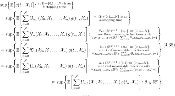
(I) A neural network architecture for in an appropriate sense ‘randomised’ stopping times (cf. (4.31) in Subsection 4.1.4) is established in such a way that varying the neural network parameters leads to different randomised stopping times being ex- pressed. This neural network architecture is used to replace the supremum of the expected pay-off over suitable stopping times (which constitutes the generic opti- mal stopping problem) by the supremum of a suitable objective function over neural network parameters (cf. (4.38)–(4.39) in Subsection 4.1.5).
(II) A stochastic gradient ascent-type optimisation algorithm is employed to compute neural network parameters that approximately maximise the objective function (cf.
Subsection 4.1.6).
(III) From these neural network parameters and the corresponding randomised stopping time, a true stopping time is constructed which serves as the approximation for an optimal stopping strategy (cf. (4.44) and (4.46) in Subsection4.1.7). In addition, an approximation for the optimal expected pay-off is obtained by computing a Monte Carlo approximation of the expected pay-off under this approximately optimal stop- ping strategy (cf. (4.45) in Subsection 4.1.7).
It follows from (III) that the proposed algorithm computes a low-biased approximation of the optimal expected pay-off (cf. (4.48) in Subsection 4.1.7). Yet a large number of numerical experiments where a reference value is available (cf. Section 4.3) show that the bias appears to become small quickly during training and that a very satisfying accuracy can be achieved in short computation time, even in high dimensions (cf. the introductory paragraph of Chapter 4 for a brief overview of the numerical computations that have been performed). Moreover, in (I) we resort to randomised stopping times in order to circumvent the discrete nature of stopping times that attain only finitely many different values. As a result it is possible in (II) to tackle the arising optimisation problem with a stochastic gradient ascent-type algorithm. Furthermore, while the focus in Chapter 4lies on American and Bermudan option pricing, the proposed algorithm can also be applied to optimal stopping problems that arise in other areas where the underlying stochastic process can be efficiently simulated. Apart from this, we only rely on the assumption that the stochastic process to be optimally stopped is a Markov process (cf. Subsection 4.1.4).
But this assumption is no substantial restriction since, on the one hand, it is automat- ically fulfilled in many relevant problems and, on the other hand, a discrete stochastic process that is not a Markov process can be replaced by a Markov process of higher di- mension that aggregates all necessary information (cf., e.g., [28, Subsection 4.3] and, e.g., Subsection 4.3.4.4).
Next we make a short comparison to the algorithm introduced in [28]. The latter is based on introducing for every point in time where stopping is permitted an auxiliary optimal stopping problem, for which stopping is only allowed at that point in time or later