Single-molecule analysis of transcription initiation in archaea and eukaryotes

Single-molecule analysis of transcription initiation in archaea and eukaryotes

Dissertation

zur Erlangung des Doktorgrades der Naturwissenschaften (Dr. rer. nat.) der Fakultät für Biologie und Vorklinische Medizin

der Universität Regensburg

Vorgelegt von

Kevin Oliver Kramm

aus Peine

Regensburg im September 2020

Das Promotionsgesuch wurde eingereicht am:

18.09.2020

Die Arbeit wurde angeleitet von:

Prof. Dr. Dina Grohmann

Unterschrift:

Parts of this thesis have been published in the following articles:

K. Kramm, T. Schröder, J. Gouge, A.M. Vera, K. Gupta, F.B. Heiss, T. Liedl, C. Engel, I. Berger, A. Vannini, P. Tinnefeld, D. Grohmann, DNA origami-based single-molecule force spectroscopy elucidates RNA Polymerase III pre-initiation complex stability., Nat.

Commun. 11 (2020) 2828.

K. Kramm, C. Engel, D. Grohmann, Transcription initiation factor TBP: old friend new questions., Biochem. Soc. Trans. 47 (2019) 411–423.

K. Kramm, U. Endesfelder, D. Grohmann, A Single-Molecule View of Archaeal Transcription, J. Mol. Biol. 431 (2019) 4116–4131.

J. Gouge, N. Guthertz, K. Kramm, O. Dergai, G. Abascal-Palacios, K. Satia, P. Cousin, N.

Hernandez, D. Grohmann, A. Vannini, Molecular mechanisms of Bdp1 in TFIIIB assembly and RNA polymerase III transcription initiation, Nat. Commun. 8 (2017) 130.

Contributions to other publications:

R.J. Buckley, K. Kramm, C.D.O. Cooper, D. Grohmann, E.L. Bolt, Mechanistic insights into Lhr helicase function in DNA repair, Biochem. J. 477 (2020) 2935–2947.

L. Jakob, T. Treiber, N. Treiber, A. Gust, K. Kramm, K. Hansen, M. Stotz, L. Wankerl, F.

Herzog, S. Hannus, D. Grohmann, G. Meister, Structural and functional insights into the fly microRNA biogenesis factor Loquacious., RNA. 22 (2016) 383–96.

S. Schulz, K. Kramm, F. Werner, D. Grohmann, Fluorescently labeled recombinant RNAP

system to probe archaeal transcription initiation, Methods. 86 (2015) 10–18.

Table of Contents VII

Table of Contents

Abstract ... 11

Zusammenfassung ... 13

1 Introduction ... 15

2 Single-molecule measurements ... 18

2.1 Single-molecule fluorescence measurements ... 18

2.1.1 Photophysics of organic fluorophores ... 18

2.1.2 Förster resonance energy transfer... 20

2.1.3 Total internal reflection fluorescence microscopy ... 23

2.1.4 Confocal fluorescence microscopy ... 25

2.2 Single-molecule force measurements ... 26

2.2.1 DNA origami-based single-molecule force spectroscopy ... 27

3 Transcription initiation ... 30

3.1 The TATA-binding protein ... 33

3.1.1 Analysis of TBP-DNA interactions with single-molecule FRET ... 35

3.2 TFIIB-like factors ... 35

3.2.1 Analysis of TFIIB-like factor mechanisms with single-molecule FRET ... 37

3.3 The central RNA polymerase III initiation factor TFIIIB ... 37

3.4 Mechanisms of transcriptional regulation in archaea ... 38

3.5 Influence of DNA strain and compaction on transcription ... 39

4 Objectives ... 43

5 Materials ... 44

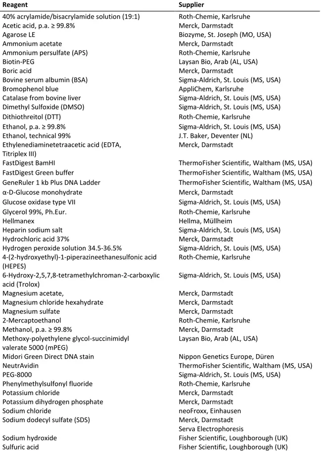
5.1 Chemicals and reagents ... 44

5.2 Buffers ... 45

5.3 Proteins ... 48

5.4 DNA oligonucleotides ... 49

5.5 Expendable items ... 50

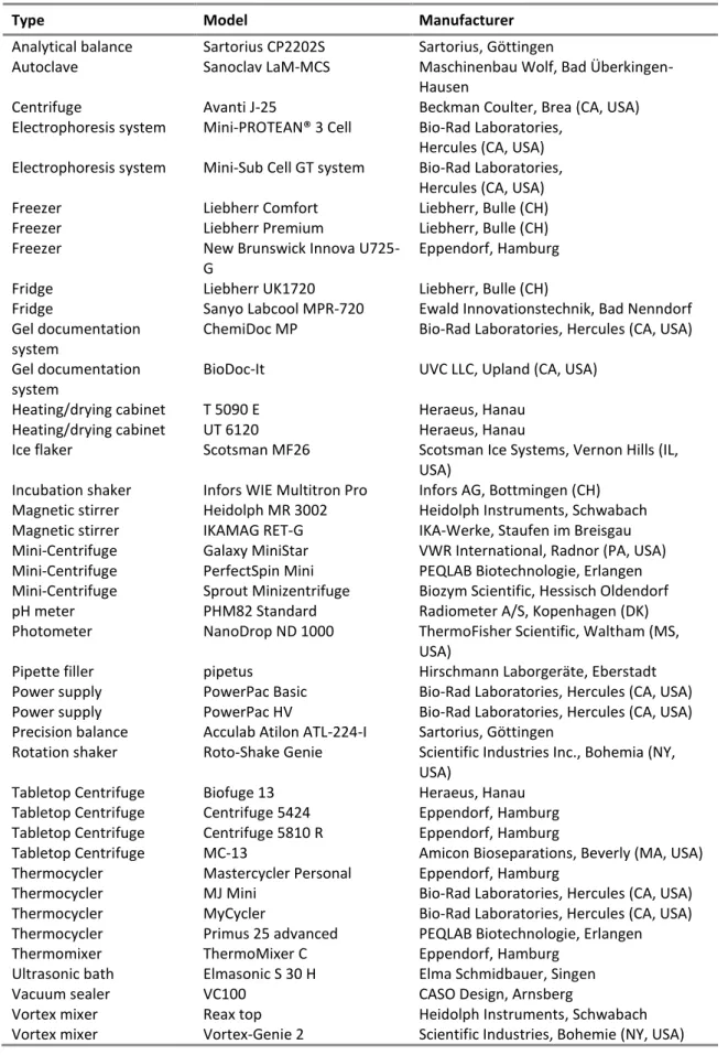
5.6 Devices ... 51

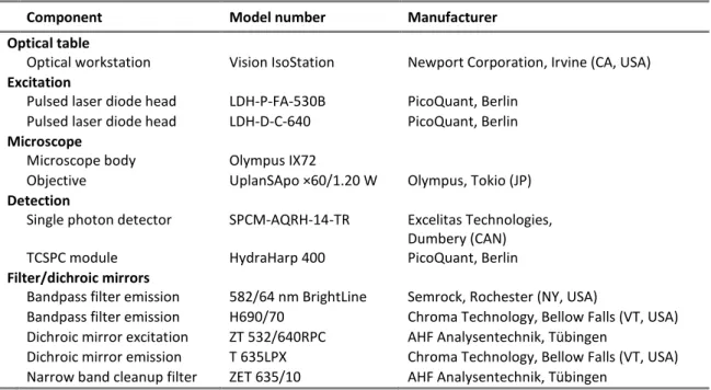
5.7 Microscope components ... 52

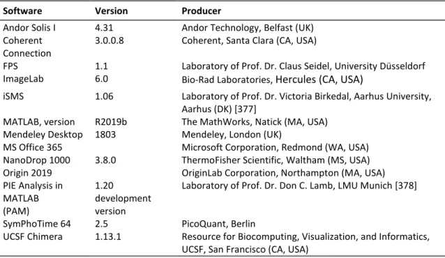
5.8 Software ... 54

6 Methods ... 55

6.1 Annealing of DNA oligonucleotides... 55

6.2 Absorption spectroscopy ... 55

6.3 Preparation of DNA origami force clamps ... 55

6.3.1 Preparation of doubly labelled promoter DNA ... 55

6.3.2 Restriction digestion of origami scaffolds ... 57

6.3.3 Thermal annealing and purification ... 57

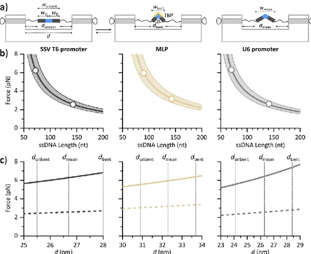
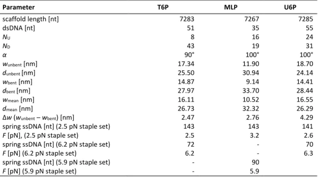
6.4 Calculation of forces for DNA origami force clamps ... 58

6.5 Transmission electron microscopy ... 61

6.6 Confocal single-molecule fluorescence microscopy experiments ... 62

6.6.1 Pulsed Interleaved Excitation ... 63

6.6.2 Diffusion-based single-molecule FRET measurements ... 63

6.7 Data analysis for confocal fluorescence microscopy experiments ... 64

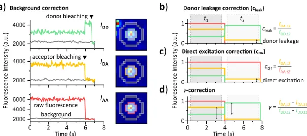
6.7.1 Calculation of correction factors ... 66

6.7.2 Calculation of FRET efficiency histograms ... 67

6.7.3 TBP-induced bending probability ... 67

6.7.4 Dwell time calculation for diffusion-based experiments ... 68

6.7.5 FRET-2CDE filter ... 69

6.7.6 Fluorescence correlation spectroscopy ... 71

6.8 TIRF microscopy experiments ... 71

6.8.1 Alternating laser excitation ... 73

6.8.2 Passivation of microscope slides ... 73

6.8.3 Flow chamber preparation ... 73

6.8.4 Photo-stabilization ... 74

6.8.5 Surface-based single-molecule FRET measurements ... 76

6.9 Data analysis for TIRF microscopy experiments... 77

6.9.1 Calculation of correction factors ... 77

6.9.2 Calculation of FRET efficiency histograms ... 79

6.9.3 Dwell time calculation from FRET efficiency-time traces ... 79

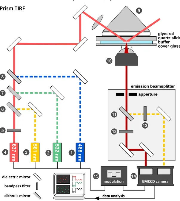
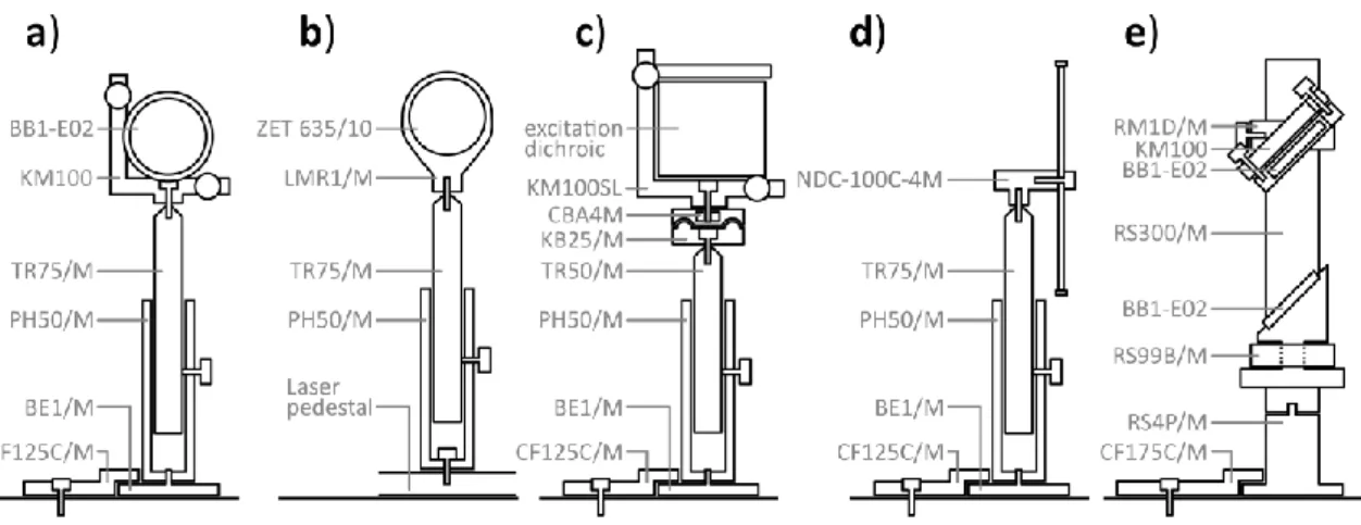
6.10 Construction of a prism-type TIRF microscope ... 81

6.10.1 Laser-combining unit ... 82

6.10.2 Illumination unit ... 84

6.10.3 Detection unit ... 86

6.10.4 Control of electronic devices ... 88

7 Results ... 89

7.1 Conformational dynamics of DNA Holliday junctions ... 89

7.1.1 Magnesium-dependent conformational dynamics of DNA Holliday junctions ... 90

7.1.2 Kinetics of isoform I–isoform II conformational dynamics ... 92

7.1.3 Role of the open conformation in Holliday junction dynamics ... 94

7.2 Assembly of human TFIIIB at the U6 snRNA promoter ... 97

7.2.1 Assembly of TFIIIB subcomplexes under equilibrium conditions ... 100

7.2.2 Stability of TFIIIB subcomplexes after depletion of unbound proteins ... 102

7.2.3 Dynamics of HsTBP-induced promoter DNA bending ... 105

7.3 Force-dependency of DNA binding by RNAP II and III transcription factors ... 108

7.3.1 Force dependency of human TBP-induced promoter DNA bending ... 112

7.3.2 Influence of RNAP II and III transcription factors on TBP-induced DNA bending ... 112

7.3.3 Influence of mechanical strain on DNA bending kinetics ... 116

7.4 Mechanisms of transcriptional regulation in archaea ... 121

7.4.1 The role of Sulfolobus acidocaldarius TFB2 in transcription initiation ... 121

7.4.2 Analysis of Pyrococcus furiosus TFB RF1-assisted transcription initiation ... 124

7.4.3 Force-dependency of DNA bending induced by archaeal transcription factors ... 128

8 Discussion ... 131

8.1 Influence of individual subunits on TFIIIB assembly ... 131

8.1.1 Influence of DNA sequence on HsTBP-induced DNA bending dynamics ... 131

8.1.2 Different DNA bending angles for U6 promoter and MLP complexes ... 133

8.1.3 Stabilization of the U6 promoter-TBP complex by Brf2 ... 135

Table of Contents IX

8.1.4 Stabilization of the U6 promoter-TBP-Brf2 complex by Bdp1 ... 135

8.1.5 Bending-angle differences between TIRF and confocal microscopy experiments ... 138

8.2 Comparison of force-dependent DNA binding by human RNAP II and III

transcription factors ... 139

8.2.1 Influence of mechanical strain on TBP-induced DNA bending dynamics ... 139

8.2.2 Stability of ternary U6 promoter and MLP complexes ... 141

8.2.3 Stability of quarternary U6 promoter and MLP complexes ... 142

8.2.4 The central FRET efficiency population in FC experiments ... 145

8.2.5 Comparison of experimental and theoretical DNA bending probabilities ... 147

8.3 The role of TFB2 in transcription initiation ... 150

8.4 Mechanism of TFB-RF1-mediated TFB recruitment ... 153

8.5 Influence of force on DNA bending induced by archaeal transcription factors ... 155

8.6 Conclusion and outlook ... 157

9 References ... 159

Danksagung ... 185

List of abbreviations ... 186

List of figures ... 188

List of tables ... 191

Appendix ... 192

A Protein sequences ... 192

B DNA origami scaffolds ... 195

C Extended data ... 197

C.1 Measurements with DNA Holliday junctions ... 197

C.2 Analysis of human TFIIIB with TIRF microscopy ... 198

C.3 Force measurements with human RNAP II and III transcription factors ... 200

C.4 Measurements with Sulfolobus acidocaldarius transcription factors ... 204

C.5 Measurements with Pyrococcus furiosus transcription factors ... 205

C.6 Force measurements with archaeal transcription factors ... 206

Abstract 11

Abstract

Transcription is the transfer of information stored in the DNA genome into RNA and an essential process for cellular life. In all three domains of life, transcription is carried out by structurally conserved RNA polymerases (RNAP). archaea employ only a single RNAP while eukaryotes have evolved three functionally distinct variants, RNAP I, II and III. Transcription is a cyclic process divided into initiation, elongation and termination phases. During transcription initiation, RNAPs are recruited to the promoter region of their target genes by transcription factors (TF) that recognize sequence elements in the promoter DNA, leading to formation of a pre-initiation complex (PIC). In archaeal and all eukaryotic transcription systems, initiation relies on the TATA- binding protein (TBP) and a TFIIB-like factor.

TFIIIB, the central initiation factor of the human RNAP III system is composed of TBP, the TFIIB- related factors Brf1 or Brf2 and the RNAP III-specific factor Bdp1. At TATA-box-containing promoters, TFIIIB alone can recruit RNAP III. In contrast, RNAP II recruitment can be achieved by TBP and TFIIB. How TFIIIB dynamically assembles at the promoter and the role of Bdp1 as an additional required factor are still not well understood. Furthermore, TFIIIB forms highly stable complexes on DNA that can persist for multiple rounds of transcription. How transcription factors are affected by mechanical forces exerted on DNA by cellular processes like transcription and DNA compaction is mostly unexplored. The archaeal transcription machinery resembles the eukaryotic RNAP II system, but gene regulation is performed by Bacteria-like transcriptional regulators. In

weak B recognition element (BRE) by binding to a conserved upstream promoter element. The molecular mechanism and potential conformational changes in the DNA are still elusive. Many archaea evolved paralogs of TBP and TFB that are involved in stress response. In

function in the context of transcription is still unexplored.

Assembly of TFs at the promoters is highly dynamic and involves TBP-induced bending of the promoter DNA by approximately 90°. This conformational change can be detected by Förster resonance energy transfer (FRET), a distance-dependent non-radiative process that can report on distance changes in the 1–10 nm regime with high time resolution. In this work, FRET measurements are performed at the single-molecule level, which allows direct observation of different conformational states of individual initiation complexes in real-time. Furthermore, force measurements were performed with a DNA origami-based nanodevice that can exert constant force in the piconewton range on a double stranded DNA fragment. To facilitate FRET experiments, a total internal reflection fluorescence (TIRF) microscope was constructed. In this work, TIRF and confocal fluorescence microscopy were used to study the molecular mechanisms underlying human and archaeal transcription initiation.

The stepwise assembly of TFIIIB at the U6 snRNA promoter was monitored, revealing transient

DNA binding of TBP on the millisecond timescale. Addition of Brf2 and Bdp1 stabilized dynamic

DNA/TBP complexes. Force measurements revealed that binding of human TFs to DNA under

mechanical strain is impaired. The complete TFIIIB complex can bind to DNA at forces up to 6.3 pN,

whereas binding of TBP and TBP/Brf2 was strongly reduced at 2.6 pN and 6.3 pN, respectively. A comparison with the RNAP II-specific TFIIB and TFIIA provides evidence that the cage-like structure of TFIIIB confers superior resistance to mechanical force.

S. acidocaldarius

TFB2 cannot stabilize a bent promoter DNA/TBP complex and is thus not functional as a transcription initiation factor. Instead, six-fold molar excess of TFB2 could destabilize a DNA-bound TBP/TFB complex, suggesting a regulatory role for TFB2.

TFB-RF1 can enhance TFB recruitment at promoters with weak or consensus BREs to similar degree without inducing conformational changes in the DNA. However, formation of a bent promoter DNA complex is slower at promoters with a consensus BRE. TFB-RF1 likely acts as a secondary binding site for TFB.

DNA origami-based force spectroscopy further demonstrated force-dependent DNA bending of archaeal TFs.

requires TBP and TFB. For both systems, low DNA bending efficiency was observed at 6.2 pN force.

Taken together, this work highlights conserved mechanisms employed by archaeal and eukaryotic

transcription systems to modulate the stability of the TBP/TFIIB-like factor complex that nucleates

PIC formation, thereby enabling control over transcription initiation.

Zusammenfassung 13

Zusammenfassung

Transkription ist der Transfer von im DNA-Genom gespeicherten Informationen in RNA und daher ein wichtiger Prozess für zelluläres Leben. Transkription erfolgt in allen drei Domänen des Lebens durch strukturell konservierte RNA-Polymerasen (RNAPs). Archaeen verwenden nur eine einzige RNAP, während Eukaryoten drei funktionell unterschiedliche Varianten entwickelt haben, RNAP I, II und III. Transkription ist ein zyklischer Prozess, der in Initiations-, Elongations- und Terminationsphasen unterteilt ist. Während der Transkriptionsinitiation wird die RNAP durch Transkriptionsfaktoren (TFs), die Sequenzelemente in der Promotor-DNA erkennen, in die Promotorregion ihrer Zielgene rekrutiert. Dies führt zur Formierung eine Prä-Initiationskomplexes (engl.: pre-initiation complex, PIC). Im archaeellen und allen eukaryotischen Transkriptionssystemen bilden das TATA-bindende Protein (TBP) und ein TFIIB-ähnlicher Faktor die Kernkomponenten der Initiation.

TFIIIB, der zentrale Initiationsfaktor des humanen RNAP III-Systems, besteht aus TBP, dem TFIIB- ähnlichen Faktor Brf1 oder Brf2 und dem RNAP III-spezifischen Faktor Bdp1. Die Rekrutierung von RNAP III kann an Promotoren mit einem TATA-box Element allein durch TFIIIB erfolgen. Im Gegensatz dazu kann die Rekrutierung von RNAP II durch TBP und TFIIB erreicht werden. Der dynamische Assemblierungsprozess von TFIIIB auf der Promotor DNA, sowie die Rolle von Bdp1 als zusätzlich erforderlichem Faktor im RNAP III System, sind noch nicht gut untersucht. Darüber hinaus bildet TFIIIB extrem stabile Komplexe mit DNA, die für mehrere Transkriptionszyklen bestehen bleiben können. Wie Transkriptionsfaktoren durch mechanische Kräfte beeinflusst werden, die durch zelluläre Prozesse wie Transkription und DNA-Kompaktierung auf die DNA ausgeübt werden, ist weitgehend unerforscht. Die archaeelle Transkriptionsmaschinerie ähnelt dem eukaryotischen RNAP II System, aber Genregulation erfolgt durch Transkriptionsregulatoren, die denen in Bakterien ähneln. Im Archaeon Pyrococcus furiosus kann TFB an Promotoren mit einem schwachen B-Erkennungselement (engl.: B recognition element, BRE) durch den TFB- Rekrutierungsfaktor 1 (TFB-RF1) stimuliert werden, der an ein konserviertes Promotorelement stromaufwärts des BRE bindet. Der molekulare Mechanismus und mögliche Konformationsänderungen der DNA sind noch nicht bekannt. Viele Archaeen haben Paraloga von TBP und TFB evolviert, die an Genregulation in Reaktion auf Stressbedingungen beteiligt sind. In

Funktion TFB2 im Rahmen der Transkriptionsinitiation spielt ist jedoch noch unerforscht.

Die Assemblierung von TFs an der Promotor-DNA ist dynamisch und eine wichtige

Konformationsänderung bei diesem Prozess ist eine durch TBP induzierte Biegung der DNA um

circa 90°. Diese Konformationsänderung kann durch Förster-Resonanzenergietransfer (FRET)

detektiert werden. FRET ist ein abstandsabhängiger, strahlungsfreier Prozess, mit dem

Abstandsänderungen im Bereich von 1–10 nm mit hoher zeitlicher Auflösung gemessen werden

können. In dieser Arbeit werden FRET-Messungen auf Einzelmolekülebene durchgeführt, wodurch

die direkte Beobachtung verschiedener Konformationszustände einzelner Initiationskomplexe in

Echtzeit möglich ist. Darüber hinaus wurden Kraftmessungen mit einem DNA Origami-basierten

Nanogerät durchgeführt, das eine konstante Kraft im Piconewton-Bereich auf ein

doppelsträngiges DNA-Fragment ausüben kann. Für FRET-Experimente wurde ein internes Totalreflektionsfluoreszenzmikroskop (engl.: total internal reflection fluorescence, TIRF) konstruiert. In dieser Arbeit wurden TIRF und konfokale Fluoreszenzmikroskopie eingesetzt um die molekularen Mechanismen der Transkription in archaeellen und eukaryotischen Transkriptionssystemen zu erforschen.

Die Untersuchung der schrittweisen Assemblierung des TFIIIB-Komplexes am U6 snRNA-Promotor zeigte, dass TBP-induzierte DNA-Biegung transient erfolgt, mit Bindungszeiten im Millisekundenbereich. Brf2 und Bdp1 können dynamische DNA/TBP-Komplexe stabilisieren.

Kraftspektroskopiemessungen ergaben, dass die DNA-Bindung humaner TFs beeinträchtigt ist, wenn mechanische Kraft auf die DNA einwirkt. Der vollständige TFIIIB-Komplex kann bei Kräften bis zu 6,3 pN an DNA binden, während die Bindung von TBP und TBP/Brf2 bei 2,6 pN bzw. 6,3 pN stark reduziert war. Ein Vergleich mit den RNAP II-spezifischen Faktoren TFIIB und TFIIA liefert Hinweise darauf, dass die käfigartige Struktur des TFIIIB-Komplexes eine hohe Beständigkeit gegen mechanische Kräfte vermittelt.

Der S. acidocaldarius Faktor TFB2 trägt nicht zur Stabilisierung eines Promotor-DNA/TBP-Komplex bei und ist daher keine funktionsfähiger Transkriptionsinitiationsfaktor. Stattdessen konnte ein sechsfacher molarer Überschuss an TFB2 einen DNA-gebundenen TBP/TFB-Komplex destabilisieren, was auf eine regulatorische Rolle für TFB2 hindeutet.

TFB-RF1 kann die TFB-Rekrutierung sowohl an Promotoren mit schwachen als auch consensus BREs in ähnlichem Maße verbessern. Dabei wurden keine Konformationsänderungen der DNA beobachtet. Die Formierung eines gebogenen Promotor-DNA-Komplexes erfolgte jedoch bei Promotoren mit consensus BRE langsamer. Es ist anzunehmen, dass TFB-RF1 als eine sekundäre Bindungsstelle für TFB am Promotor fungiert.

DNA-Origami-basierte Kraftspektroskopie zeigte ferner, dass DNA-Biegung durch archaeelle Transkriptionsfaktoren kraftabhängig ist.

biegen, während im

Systeme war bei einer an der DNA anliegenden Kraft von 6,2 pN die Effizienz der DNA-Biegung stark reduziert.

Zusammengenommen beleuchtet diese Arbeit konservierte Mechanismen, die von archaeellen

und eukaryotischen Transkriptionssystemen genutzt werden um die Stabilität des TBP/TFIIB-

ähnlichen Faktor-Komplexes zu modulieren, der den Kern des PIC bildet, wodurch Kontrolle über

die Transkriptionsinitiation ermöglicht wird.

Introduction 15

1 Introduction

Single-molecule techniques have reshaped our view on cellular life over the last decades. The molecular machines that perform the most fundamental processes within living cells such as DNA replication, transcription and translation are highly dynamic by nature. Just as in large scale machines, movement of individual components

functionality and understanding the underlying molecular mechanism is the key to understanding cellular life itself (reviewed in [1–3]). The concept of interrogating such complex systems one molecule at a time presents unique advantages over classical ensemble approaches:

Probing individual molecules provides information on the distribution of values for a given property, e.g. structural conformation, whereas averaging over an ensemble only reflects the mean value of the observed parameter. Thus, single-molecule approaches can reveal molecular heterogeneity, which is an intrinsic feature of biological systems. A theoretical example for this is provided by a protein that can exist in two different conformational states that differ in the distance between two domains (Figure 1a). In an ensemble experiment, only the mean distance can be measured. This value does not correspond to either conformation and only reflects the relative fraction of each conformer in the heterogeneous ensemble. On the other hand, probing individual molecules also yields the relative fraction of each conformer, but more importantly provides information on the mean distance and its variance for each separate conformational state. If the state of each molecule remains constant over the timespan of the observation, such a system displays static heterogeneity.

Figure 1: Concepts of molecular heterogeneity. a) Static heterogeneity is observed in a sample by probing the conformational state (distance between red and blue domain) of individual molecules. This approach captures the distribution of distance values in a sample. In contrast, measuring the sample in an ensemble approach only recovers the mean distance resulting from the relative fraction of each conformer in the ensemble (here 1:1). b) Dynamic heterogeneity is observed for a molecule that fluctuates between three conformational states in a stochastic manner.

In contrast, dynamic heterogeneity is observed if the conformation of the molecules can change

over the timespan of the observation. Conformational transitions can be divided into two

categories. The first are unidirectional transitions, e.g. the unfolding of a single protein [4]. These

changes are per se also accessible to ensemble methods as they can in some instances be

synchronized, i.e. the initial and final state are respectively identical for each molecule in the

ensemble. The second category are recurring transitions that occur in a stochastic manner and are

thus inherently non-synchronizable (Figure 1b). These processes are generally inaccessible to

ensemble methods but constitute the majority of biomolecular motions [5]. By employing a single- molecule approach, the conformational transitions in a molecule can be followed in real-time providing information on the order and relative occurrence of individual steps as well as the dwell time of the molecule in each specific state (Figure 1b). In this manner, rare subpopulations of molecules can be discovered and interrogated [6]. Consequently, molecules can be further sorted to focus downstream data analysis on only on relevant subpopulations. Hence, single-molecule methods provide a wealth of information and enable unique strategies to approach biochemical and biophysical questions.

The detection of single molecules can be achieved by several means (reviewed in [7]): changes in electrical current (patch clamp and nanopore DNA sequencing [8]), local differences in electronic transmittance (electron microscopy) or exerted forces (atomic force microscopy (AFM), optical and magnetic tweezers [9,10]). But for biological applications, optical detection schemes have proven to be the most versatile (reviewed in [11]). In particular fluorescence provides a readout parameter well suited for biological samples as fluorescent proteins can be genetically fused to a protein of interest in living cells [12,13]. Organic fluorophores, on the other hand, can be covalently attached to proteins and nucleic acids through a plethora of chemical reactions, many of which are suitable for application in living cells [14,15] (reviewed in [11,16,17]).

Single-molecule fluorescence experiments involving biological samples encounter two main challenges (reviewed in [11,16,18]). First, sensitivity to the fluorescence emission of a single molecule must be achieved. Autofluorescence and light scattering within the sample can cause significant background signals that can dominate the combined signal [19]. Thus, reliable detection of single molecules depends on either signal amplification [20,21] or background reduction [22–25]. The most commonly utilized methods for single-molecule fluorescence experiments are confocal [22,26] and total internal reflection fluorescence (TIRF) microscopy [25,27], which both rely on limiting the detection volume and thereby reducing the contribution of background signal. Secondly, single-molecule methods generally operate at extremely low concentrations (picomolar to nanomolar) to achieve spatial separation between particles [18].

However, many biological systems often have considerably higher dissociation constants (K

) [18].

This concentration barrier dictates that only biological interaction of labeled reactants with K

values below 50 nM are accessible to single-molecule techniques [16].

As stated above, the detection of conformational changes in individual biological complexes is one

of the main aims of single-molecule approaches in life sciences. Distance information in the

biologically relevant regime of 1–10 nm can be obtained in single-molecule fluorescence

measurements by exploiting a phenomenon termed Förster resonance energy transfer (FRET)

[28,29]. FRET is a form of non-radiative energy transfer from a fluorescent donor molecule to an

acceptor. The efficiency of this process is highly distance-dependent and requires donor and

acceptor to be in close proximity (1–10 nm). By measuring the FRET efficiency between two

strategically placed fluorophores within a biomolecular complex, distances and distance changes

can be monitored [30,31]. Hence, single-molecule FRET experiments (smFRET) can identify distinct

structural states of a biological macromolecule and detect transient or rare species. In contrast to

classical structural biology methods such as x-ray crystallography or cryo-electron microscopy,

Introduction 17

these data are attainable at high time-resolution, allowing real-time observation of entire conformational cycles (reviewed in [2,32–35]).

SmFRET experiments have been variously applied to study the molecular mechanism of cellular processes such as DNA replication [36–39] and mRNA translation [40–43]. In this work, the focus is set on transcription, the transfer of the genetic information encoded in the DNA genome into RNA. Transcription is the first step in gene expression and this task is carried out by structurally conserved multisubunit RNA polymerases (RNAPs) in all three domains of life – Bacteria, Archaea and Eukarya [44]. While bacteria and archaea rely on a single RNAP, eukaryotes have evolved three functionally distinct variants, RNAP I, II and III. RNAP I exclusively synthesizes ribosomal RNA (rRNA), performing the bulk of transcription activity in dividing cells [45]. RNAP II primarily produces messenger RNAs (mRNA) that are translated into proteins, as well as regulatory RNAs and small nuclear RNAs (snRNA). RNAP III transcribes short structured RNAs such as transfer RNAs (tRNA), the 5S rRNA and the U6 snRNAs. These molecular machines consist of an evolutionary conserved five-subunit core complex that harbors the catalytic center of the RNAP. In archaea and eukaryotes, this core complex is extended by additional 7–12 subunits that share functional and structural features (reviewed in [44,46]).

Transcription is a cyclic process that can be divided into the initiation, elongation and termination phases. During the initiation phase, the RNAP binds the promoter DNA upstream of a target gene and separates the DNA duplex. In the elongation phase, the RNAP translates along the gene body and synthesizes an RNA complementary to the DNA matrix via nucleoside triphosphate hydrolysis.

In the termination phase, the RNAP releases the transcribed RNA and disengages the DNA. These steps are supported by a multitude of accessory proteins dynamically associating with the promoter DNA and RNAP to induce conformational changes that are critical for RNAP functionality and progression through the transcription cycle (reviewed in [47]).

During the initiation phase, the RNAP must bind to the promoter region of a gene, separate (“melt”) the DNA duplex and position the transcription start site (TSS) in the active center. To achieve this, RNAPs are aided by transcription factors (TFs) that assist in promoter recognition, precise RNAP positioning and DNA melting. In Bacteria, σ factors bind to the RNAP in solution to form a holo-enzyme. This complex can bind to different target promoters depending on the bound

the TATA-binding protein (TBP) that binds to the TATA-box element of the promoter, thereby inducing a sharp bent in the DNA and a TFIIB-like factor that recruits the RNAP to the promoter, forming a pre-initiation complex (PIC) [51–53]. This core arrangement is generally conserved and expanded by additional RNAP-specific factors (reviewed in [46,54]).

While snapshots of these intermediate assemblies have been attained by classical structural

biology approaches (reviewed in [55,56]), real time-observation provides a more nuanced picture

of this highly dynamic process. Hence, single-molecule experiments are the preferred choice to

unravel the molecular mechanisms underlying transcription that have expanded our knowledge

over the past decades (reviewed in [57–60]). In this work, several aspects surrounding the

mechanisms of transcription initiation in eukaryotes and archaea will be addressed by harnessing

the power of the single-molecule FRET toolbox.

2 Single-molecule measurements

2.1 Single-molecule fluorescence measurements

Optical single-molecule measurements can provide detailed insights into biological processes.

Fluorescence serves as a sensitive reporter that provides information on changes in the environment of the fluorophore such as pH value [61], temperature [62], viscosity, and the vicinity of other molecules (e.g. FRET [28] (Chapter 2.1.2), protein induced fluorescence enhancement [63]) or surface proximity (metal induced energy transfer [64]). In this section, a theoretical background on the single-molecule fluorescence microscopy methods applied in this work is provided.

2.1.1 Photophysics of organic fluorophores

Fluorophores are molecules that contain delocalized π-electrons, which can absorb light with a wavelength λ in the ultraviolet to near infrared spectrum. The energy E

of absorbed photons is described by:

𝐸_photon= ℎ ∙𝑐

𝜆 Equation 1

where

then be released via emission of light, which is termed luminescence. The processes that occur between the absorption and emission of light by fluorophores, and their respective rates k, are usually visualized in a Jablonski diagram (Figure 2).

Initially, the fluorophore is in the singlet ground state S

. Upon absorption of a photon with an energy equal or higher than the energy barrier of the first (S

) or second excited singlet state (S

), the fluorophore is shifted to the respective state. The transition is near instantaneous (k

≈ 10

s

), and the excited electron is usually shifted to a higher vibrational level of the S

or S

state, where it is spin-paired with the electron in the S

state. From there, the molecule quickly transitions to the lowest vibrational level of that state by vibrational relaxation under dissipation of heat (k

≈ 10

s

). If overlap exists between the vibrational levels of two electronic states, the molecule can relax to the lower state in a process termed internal conversion (k

= 10

s

).

Internal conversion is more likely to occur in the S

transition than the S

transition due to the larger energy difference of the latter. From the relaxed S

state, further relaxation to S

can occur via emission of a photon as fluorescence, a subtype of luminescence. This transition is spin allowed and can therefore proceed rapidly (k

≈ 10

s

). Alternatively, excited electrons in the S

state can undergo spin-conversion to the first excited triplet state T

in a process called inter system crossing (k

= 10

s

). From this state, the molecule can also radiatively return to S

by emitting phosphorescence. This transition is spin-forbidden and is several orders of magnitude slower than fluorescence (k

≈ 10

s

). Additional non-radiative relaxation pathways exist, such as collision quenching, complex formation and resonance energy transfer [65,66]

(Chapter 2.1.2). Both radiative relaxation processes usually lead to a decay to a higher vibrational

level of S

. From there, excess energy is dissipated via vibrational relaxation.

Single-molecule measurements 19

The energy losses incurred from intermediate relaxation pathways decrease the energy available for radiative relaxation. Thus, fluorescence and phosphorescence occur at a longer wavelength than the absorbed light, an effect termed Stokes shift. This phenomenon can be exploited in technical applications to achieve spectral separation of excitation and emission photons.

The number of photons emitted as fluorescence versus the total amount of absorbed photons (or the total amount of deexcitation events) is defined as the fluorescence quantum yield Φ

.

𝛷_fl= 𝑘_fl

𝑘_fl+ 𝑘_nr Equation 2

where

is the sum of all non-radiative rates competing for S

depopulation. Conversely, the average time a molecule spends in the excited state prior to fluorescence emission is defined as the fluorescence lifetime τ

of the fluorophore:

𝜏_fl= 1

𝑘_fl+ 𝑘_nr Equation 3

Fluorescence lifetimes are usually in the range of 1–10 ns. Fluorescence emission is a stochastic process, that can be described by an exponential decay model:

𝑁_F*(𝑡) = 𝑁_{F*, 0}∙ 𝑒⁻

𝑡

𝜏_fl Equation 4

where N

(t) is the number of excited state fluorophores at time point t after excitation and N

(t) is the total number of excited fluorophores. Thus, at t = τ

on average, 63% of all fluorophores in a simultaneously excited ensemble have returned to the ground state.

Figure 2: Simplified Jablonski diagram. A fluorophore in the electronic ground state S0 is excited to the first (S1) or second (S2) excited singlet state via absorption (kabs) of a photon. The molecule relaxes to the lowest excited vibrational level by vibrational relaxation (kVR). From there, the molecule can relax radiatively via emission of fluorescence (kfl). Overlapping vibrational levels (thin gray lines) and electronic states (thick gray lines) allow the molecule to relax non radiatively via internal conversion (kIC). Alternatively, the molecule can undergo inter system crossing (kICS) to the first triplet state T1 and radiatively relax by emission of phosphorescence (kpho). Additional non-radiative relaxation pathways are included in knr. The electron spin configuration of the ground state, first and second excited states (bottom to top) are indicated by boxed arrows. Rates are given in s^-1.

2.1.2 Förster resonance energy transfer

An alternative route for excited state depopulation is Förster resonance energy transfer, named after Theodor Förster who developed the theoretical framework around this photophysical phenomenon [28,67,68]. FRET is a non-radiative transfer of energy from an excited state donor fluorophore to a ground state acceptor molecule via dipole-dipole interaction [28]. For FRET to occur, several conditions must be fulfilled [69]:

1) Donor and acceptor must be in close, but not too close, vicinity (1–10 nm).

At closer distances, contact-based energy transfer mechanisms become prevalent such as collision quenching and complex formation between donor and acceptor [70]. It must be noted that for biological applications, fluorophores are generally attached to flexible linkers, around 1–1.5 nm in length. In praxis, inter-fluorophore contacts can already occur in the 0–3 nm distance regime [71].

At greater distances, reabsorption can be observed, wherein a photon emitted by the donor is subsequently absorb by the acceptor and elicits acceptor fluorescence. Depending on the experimental setup, the above phenomena can macroscopically be interpreted as FRET but operate through entirely different mechanisms [70].

2) Spectral overlap is required between the donor emission the acceptor absorption.

As a simplification, donor and acceptor fluorophores can be visualized as groups of electrical oscillators, each consisting of a stationary nucleus and an electron that can oscillate along one direction. The donor and acceptor transition dipole moments each point from the center of the respective molecule along its positive-negative charge gradient generated by the sum of all internal oscillators [72]. Spectral overlap includes that the donor emission dipole moment and acceptor absorption dipole moment oscillate at wavelengths that can resonate with each other.

This can be visualized by the intersection of the respective spectra (Figure 3). The spectral overlap is defined as the overlap integral J (Figure 3):

𝐽 = ∫ 𝑓_D(𝜆) ∙ 𝜀_A(𝜆) ∙ 𝜆⁴ d𝜆 Equation 5

where f

(λ) is the area-normalized donor fluorescence spectrum, and ε

(λ) is the molar extinction spectrum of the acceptor (in M

cm

) integrated over the spectral range.

Figure 3: The spectral overlap integral J. Absorption (abs.) and emission spectra (em.) of the FRET donor- acceptor fluorophore pair ATTO 532 and ATTO 647N, normalized to 1. The area shaded in yellow is the overlap integral JDA as a function of the wavelength. OLI: overlap integral units (10^-14 mol^-1 dm³ cm³).

Single-molecule measurements 21

3) Donor and acceptor dipoles must be in suitable alignment to each other.

In addition to spectral overlap, resonance between both dipole moments is dependent on their angular relation, defined as the orientation factor κ²:

𝜅² = (cos 𝜃_T− 3 cos 𝜃_D∙ cos 𝜃_A)²

where

is the angle between the donor emission transition dipole moment and the donor- acceptor connection line,

is the angle between the acceptor absorption transition dipole moment and the donor-acceptor connection line and ϑ

is the angle between the transition dipole moments of donor emission and acceptor absorption (Figure 4). Extreme values of

observed for collinear orientation of both transition dipole moments (ϑ

becomes 4 and orthogonal orientation (ϑ

and ϑ

over all possible orientations yields κ² = 2/3 (Figure 4). This approximation requires both fluorophores to be in isotropic rotation at a rate much faster than the rate of energy transfer[69].

When one of the dipoles is fixed in a static orientation while the other can freely rotate, κ² takes on values from 1/4 to 3/4, which is still reasonably approximated by 2/3 in most cases.

Figure 4: The orientation factor κ². ϑD and ϑA

are the angles between the donor-acceptor connection line (black) and the donor emission transition dipole moment (green arrow) or acceptor absorption transition dipole moment (red arrow). ϑT is the angle between the planes defined by ϑD and ϑA (gray dashed line). The extrema of κ² for collinear (top) and orthogonal (middle) orientation of the dipole moments, as well as the average obtained for fast isotropic rotation of fluorophores (bottom) are depicted.

If the above conditions are fulfilled, a donor residing in the S

excited state can transfer its energy to the acceptor, thereby returning to the ground state. Simultaneously, the acceptor is excited to the S

state and can return to S

either non-radiatively or via emission of fluorescence (Figure 5a).

Thus, acceptor emission upon donor excitation can be observed. The efficiency of the energy transfer E is defined as:

𝐸 = 𝑘_T

𝑘_T+ 𝜏_fl,D⁻¹= 𝑅₀⁶

𝑅₀⁶+ 𝑟_DA⁶ Equation 7

Where k

is the energy transfer rate, τ

is the fluorescence lifetime of the donor fluorophore, r

is the distance between the donor and acceptor.

is the Förster radius, at which the energy transfer efficiency is exactly 0.5. R

contains the spectral overlap and orientation conditions as:

𝑅₀=9(ln 10) ∙ 𝜅²∙ 𝜙_D∙ 𝐽

128𝜋⁵∙ 𝑁_A∙ 𝑛⁴ Equation 8

where N

is the Avogadro constant and

dependence of

regime

(Figure 5b). Values for R

are typically between 3–6 nm (see [69] for a comprehensive list), which

is ideal to study protein and nucleic acid structures. Hence, FRET is often used as

Experimentally, measuring FRET can be approached by multiple strategies that all employ common basic principles.

i) FRET is detectable as change in τ

. Since FRET provides an additional pathway for excited state depopulation, the donor fluorescence lifetime in the presence of an acceptor

is reduced compared to the isolated donor τ

, which can be exploited to calculate E as:

𝐸 = 1 −𝜏_fl,DA

𝜏_fl,D Equation 9

ii) Alternatively, using fluorescence intensity as a readout parameter, FRET is detected as quenching of donor fluorescence in the presence of an acceptor compared to the isolated donor.

iii) The emission of acceptor fluorescence upon donor excitation (acceptor sensitization) measured in the presence or absence of a donor provides information on E. The first and second approach offer the flexibility of using a non-fluorescent quencher as acceptor [74]. However, numerous deexcitation processes can lead to quenching of donor fluorescence lifetime or intensity, making this readout alone unreliable if the presence of an acceptor cannot be confirmed. Thus, in praxis, a combination of all the above principles is favored. The single- molecule techniques employed in this work offer the unique advantage of measuring all the above quantities simultaneously whilst also confirming the presence of an acceptor via direct excitation.

Thus, all parameters for accurate calculation of

(Chapters 6.6.1 and 6.8.1).

Figure 5: Principles of Förster resonance energy transfer. Simplified Jablonski diagram representing the excitation of a donor fluorophore from the electronic ground state S0 upon absorption of a photon (kabs) to the first excited singlet state S1, followed by internal conversion to the lowest vibrational level of S1 (black dashed arrow). Relaxation to S0 can occur via emission of fluorescence (kfl), non-radiative decay (knr, Figure 3) or Förster resonance energy transfer (kFRET). For FRET to occur, the energy difference of the donor S1–S0 transition must be equal to the S0–S1 transition of the acceptor (depicted as connected yellow arrows).

After FRET, the acceptor is in the excited state and can relax via emission of fluorescence or non-radiative decay. b) FRET efficiency as a function of donor-acceptor distance rDA (donor: ATTO 532, acceptor:

ATTO 647N). R0 is the Förster radius at which the FRET efficiency is 0.5 (R0, ATTO 532–ATTO 647N = 5.9 nm). FRET is sensitive to distance changes in the 0.5R0-2R0 range (modified from [69]).

Single-molecule measurements 23

2.1.3 Total internal reflection fluorescence microscopy

A powerful technique to realize single-molecule observation is total internal reflection fluorescence (TIRF) microscopy, that provides a high signal-to-background ratio by limiting excitation to a 100–300 nm section of the sample. This selective illumination is achieved by the total internal reflection of the incident excitation laser beam at the sample interface which creates an evanescent light field.

Light striking the

refractive indices n

and n

at an incidence angle ϑ

is refracted at an angle ϑ

following Snell’s law:

𝑛₁sin 𝜃₁= 𝑛₂sin 𝜃₂ Equation 10

When transitioning into a medium of lower refractive index (n

> n

), light is refracted towards the boundary. At a certain incidence angle, termed critical angle ϑ

(Equation 11), ϑ

reaches the maximum value of 90°. For incidence angles larger ϑ

, refraction no longer occurs and light is instead totally internally reflected (Figure 6a).

𝜃_crit= arcsin𝑛₂

𝑛₁ Equation 11

Simultaneously, an evanescent wave forms at the interface and propagates along the boundary in the relative direction the incident beam. The evanescent field intensity I decays exponentially with increasing distance z from the interface plane (Figure 6b) according to:

𝐼(𝑧) = 𝐼₀∙ 𝑒^{− 𝑧𝑑}

where I

is the intensity of the evanescent field at z = 0, and d is the penetration depth given by:

𝑑 = ^𝜆

4𝜋∙ √𝑛₁²∙ (sin 𝜃₁)²− 𝑛₂²

increases and is dependent on the wavelength of the excitation beam, e.g. for light striking a quartz/water interface (n

= 1.46, n

= 1.33) at an incident angle of 72°, the resulting penetration depth is

excitation (Figure 6c).

depends on the incidence angle and the polarization of the excitation beam I

,with the p-polarized components I

and the s-polarized component I

, according to:

𝐼₀^∥= 𝐼₁^∥

4 cos²𝜃₁(2 sin²𝜃₁−𝑛₂² 𝑛₁²) 𝑛₂⁴

𝑛₁⁴cos²𝜃₁+ sin²𝜃₁−𝑛₂² 𝑛₁²

Equation 14

𝐼₀^⊥= 𝐼₁^⊥4 cos²𝜃₁ 1 −𝑛₂²

𝑛₁²

Equation 15

Equation 14 and Equation 15, plotted for the above quartz/water example in Figure 6d, illustrate

that the evanescent field intensity can be 4–5 times stronger than the excitation wave for

incidence angles close to as ϑ

Figure 6: Principles of total internal reflection fluorescence microscopy. a) Light striking the interface of two media with refractive index n is totally internally reflected if the angle of incidence ϑ1 is larger than the critical angle for total internal reflection ϑcrit. The resulting evanescent field intensity decays with increasing distance z along the z-axis (green curve). b) Evanescent field intensity I as a function of z compared for different excitation wavelengths and incidence angles. c) Penetration depth d as a function of ϑ1. d) Evanescent field intensity at the boundary I0 as a function of ϑ1 for p- (I₁^∥) and s-polarized (I1⊥) excitation.

Arbitrary units (a.u.) are multiples of incident beam intensity I1. Interface media: n1,quartz = 1.46, n2,water = 1.33)

In a TIRF microscope, an evanescent field is created at the boundary of the microscope slide (or cover glass) and the sample phase, usually an aqueous buffer, to selectively excite a thin (100–

300 nm) section of the sample close to the phase boundary. Compared to epi-fluorescence microscopy, where the entire sample volume (10–100 µm) is excited and emits fluorescence, this improves the signal-to-background ratio by a factor of 100–1000. In a sufficiently diluted sample, only molecules tethered directly to the surface of the microscope slide are excited, allowing the observation individual particles. With this technique, immobilized particles can be monitored over extended periods of time. TIRF microscopy is realized by two main approaches to evanescent field geometry: one is objective-based, and one is prism-based.

In objective based TIRF microscopes, light is directed to the sample and collected from it by the objective lens. To achieve total internal reflection, the excitation light must exit the objective at an angle ϑ

from the optical axis larger than ϑ

as a parallel beam, allowing uniform reflection.

For this, the excitation laser is focused at the back focal plane of the objective and displaced

refracted at an angle determined by the numerical aperture NA, that defines the maximum half-

angle α at which the objective can receive, or in this case, transmit light as:

Single-molecule measurements 25

𝑁𝐴 = 𝑛 sin 𝛼 Equation 16

To achieve an incidence angle suitable for total internal reflection, a high NA objective, typically

from the sample, the reflected excitation beam is also efficiently collected by the objective and must be removed using suitable filters. This reduces the emission photon yield which can be problematic for weakly fluorescent samples.

In prism based TIRF microscopy, the excitation beam is directed towards the interface through a prism connected to the microscope slide by a medium of similar refractive index, e.g. immersion oil or glycerol. This configuration, introduced by Daniel Axelrod in 1981 [27], allows for a large incidence angle, resulting in a thin evanescent field (Equation 12) and consequently a high signal- to-background ratio. Emitted fluorescence is subsequently collected by an objective opposite of the excitation field. Thus, the reflected beam is excluded from the detection path. For cell and tissue imaging, this poses a disadvantage due to the need to focus trough the specimen, leading to spherical aberrations caused by diffraction within the sample. Single-molecule application are largely unaffected by this, as the sample volume is usually an isotropic aqueous phase, and the benefit of reduced background signal is appreciated. Compared to the objective-based approach, access to the sample, sandwiched between objective and prism, is limited and a specialized sample chamber is required to adjust buffer conditions during the experiment (Chapter 6.8.3).

Figure 7: Comparison of TIRF microscope geometries. In a prism-based TIRF microscope, the excitation beam is directed to the sample by a prism and totally internally reflected, if the angle of incidence is greater than the critical angle ϑcrit. The angle of incidence can have any value between ϑcrit and 180°. Fluorescence emitted by surface tethered fluorescent molecules (orange arrow) is collected by the objective opposite of the prism. b) In an objective-based TIRF microscope, the excitation beam is focused through the back focal plane and refracted by an objective with a high numerical aperture (NA =n∙sin α). The range of incidence angles is limited to values between ϑcrit.to α. The emitted fluorescence is collected on the same side as the excitation field (adapted from [75]).

2.1.4 Confocal fluorescence microscopy

Confocal fluorescence microscopy achieves a high signal-to-background ratio by axial confinement

of the excitation beam and by blocking out-of-focus emission [22,26]. To achieve the first, the

excitation laser beam is focused through the objective to a diffraction-limited spot in the sample

plane. The focused beam penetrates the entire sample along the z-axis and the emitted

fluorescence is collected by the same objective and focused on a micrometer-sized pinhole. By

this, out-of-focus emission is physically blocked. Depending on the wavelength of the excitation

laser and diameter of the pinhole the resulting confocal observation volume can be limited to approximately one femtoliter (Figure 8).

Confocal microscopy is suitable for single-molecule experiments with samples immobilized to a surface or freely diffusing particles in solution. The latter requires a sufficiently low sample concentration (1–100 pM) to ensure that the confocal volume is only ever occupied by a single particle. This approach offers the advantage of removing potential interactions of the charged glass surface with proteins and nucleic acids. Depending on diffusion speed of the sample, the transit time through the confocal volume is approximately 0.5–5 ms. During its transit, a fluorescent particle is continuously excited and emits photons (10

) that are detected as a

“burst” in signal intensity by an avalanche photo diode (APD). These devices are characterized by

high time resolution (on average 200 ps) high photon detection efficiency (on average 70%) and offer single-photon sensitivity.

Figure 8: Principles of confocal fluorescence microscopy. The excitation beam is focused through the objective into a diffraction limited spot. Diffusing molecules (gray spheres) transitioning through the excitation beam emit fluorescence (orange spheres). Emission is collected by the same objective and focused on a pinhole that block out-of-focus emission (dotted and dashed gray line). Only emission close to the focal plane (orange line) can reach the avalanche photodiode (APD), creating a confocal volume (green circle) defined by the excitation beam width and the pinhole diameter.

2.2 Single-molecule force measurements

Forces play a fundamental role in cellular processes like transcription [76–78], DNA replication

[79,80] and translation [42,81] as well as mechanisms of DNA compaction [82–85]. The most

widely employed methods for force application and sensing in biological systems are optical and

magnetic tweezers as well as AFM (reviewed in [86]). In magnetic tweezer measurements, the

molecule of interest is tethered to a surface on one end and to a magnetic particle (0.5–5 µm) on

the other. Force is applied by an electromagnet positioned above the sample [87]. Similarly,

optical tweezers trap a dielectric particle in the diffraction limited spot of a focused laser beam

[10]. The molecule of interest is tethered to the trapped particle on one end and either to a surface

or another trapped particle on the other end [88–90]. Displacement of the particle from the laser

focus exerts a restoring force that pulls the particle towards the focus [10]. In AFM experiments,

force sensing and application is facilitated by a cantilever equipped with a monomolecular tip. This

Single-molecule measurements 27

requires the molecule of interest to be tethered to the cantilever and a surface while force is applied by displacing the sample relative to the cantilever, e.g. via a piezoelectric stage [9].

These methods fill specific niches depending on the required temporal, spatial and force resolution. AFM provides high spatial resolution (approximate 1 nm) but is limited in force resolution below 10 pN, which is relevant for many biological processes (Chapter 3.5). While optical tweezers can, in principle, resolve single base pair steps in RNAP transcription (< 0.5 nm) [91], they can only measure few molecules at once, limiting experimental throughput [92]. Magnetic tweezers, on the other hand, are both force sensitive and multiple immobilized complexes can be imaged at once, but their spatial resolution is limited to approximately 5 nm. Additionally, long linkers are usually required in the above techniques that connect the system of interest to a surface or large particle, thereby introducing considerable noise and drift [93]. Moreover, surface connectors do not permit

circumvent these limitations, force application and sensing devices that are not connected to the macroscopic world have been constructed by exploiting DNA nanotechnology [94–97].

2.2.1 DNA origami-based single-molecule force spectroscopy

In DNA nanotechnology, DNA is repurposed from a carrier of genetic information to a building material for the construction of nanometer scale structures [98]. This can be realized by the DNA origami technique that was introduced 2006 by Paul Rothemund and named in analogy to origami, the art of folding a sheet of paper into a two- or three-dimensional structure [99]. Likewise, DNA origami is the process of molecular self-folding of a prescribed structure using a long, circular ssDNA (scaffold) and hundreds of short single-stranded DNA (ssDNA) oligonucleotides. These so- called staple strands, typically 20–60 bp long, are designed to bind to complementary regions of the scaffold DNA, thereby connecting (“staple”) distal parts into an organized structure.

(Figure 9a). DNA presents in ideal construction material due to the inherent complementarity of Watson-Crick base pairing, which allows self-assembly of origami structures. Hence, all necessary components can be combined in a single reaction.

Figure 9: Principles of DNA origami. a) Self-folding of a DNA origami structure from a circular ssDNA scaffold and 20-60 nt complementary staple strands. b) Schematic representation of strand cross-over in planar helix monolayers. Watson-Crick base-pairings are indicated as connecting lines between scaffold and staples;

DNA helices are depicted as gray cylinders. c) Honeycomb structure of three-dimensional DNA origami constructs. Strand crossovers are indicated by connected dots. Slices represent possible combinations of interconnection with a 21 bp periodicity (adapted from [100,101]).

After heating, the origami anneals (“folds”) based on thermodynamic stability of individual base

pairings. Thus, staple strands can be added in high excess, as strands that are only partially complementary to a scaffold region will be displaced by the correct strand during the cooling process. This enables a high yield of fully folded DNA origami structures and simplifies downstream processing.

The first DNA origami structures utilized the circular single-stranded M13mp18 phage genome (7249 nt) as a scaffold [99]. The design principle of these constructs was to connect neighboring helices via strand cross-overs every 8 bp, resulting in a 180° angle between helices (Figure 9b).

These helix monolayers were relatively flexible and only allowed construction of two-dimensional structures. In order to realize three dimensional objects, Douglas et al. introduced a honeycomb structure, wherein each helix is connected to three adjacent ones at a 120° angle every 7 bp (Figure 9c). Due to the tight packing of negatively charged phosphates in the DNA backbone, these DNA origami structures require high concentrations of Mg

ions to remain stable.

A great advantage of DNA origami is that every position in the scaffold can be specifically addressed by base complementarity. Thus, chemical modifications such as fluorophores or biotins, covalently linked to staple strands, can be precisely positioned within a structure. This enables the construction of functional nanometer scale devices (reviewed in [102]).

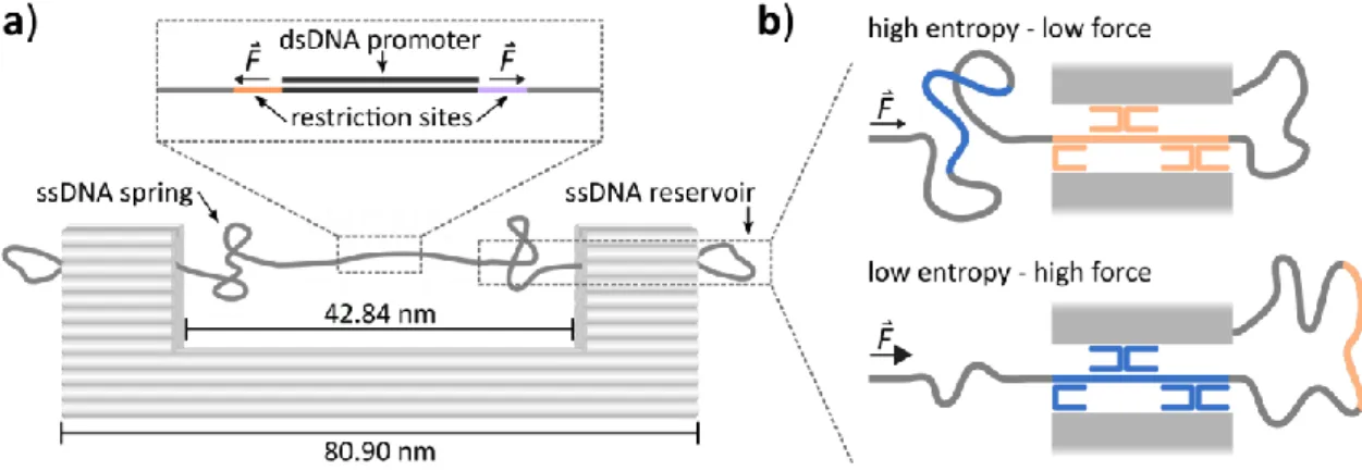
This technique was utilized recently to construct nanoscale structures that enable force application to biological samples [94,95]. Force measurements on DNA/protein complexes performed in this works were conducted using a DNA origami-based nanodevice designed by Nickels et al. [94]. This construct exploits the entropic force generated by a constrained ssDNA chain to exert a constant force in the piconewton range on a system of interest fixed within the spring. In convention with other constant force application techniques this device is termed DNA origami force clamp (FC). The FC has already been applied to study the force-dependency of conformational fluctuations in small DNA structures as well as DNA bending by TBP [94].

Figure 10: The DNA origami force clamp. a) Schematic depiction of the DNA origami force clamp structure.

Gray cylinders represent DNA helices. The inset shows the multiple cloning site of the M13mp18 phage scaffold with a cloned target sequence (here: promoter sequence) annealed to a complementary strand to form a dsDNA probe segment that is under constant force F applied by the entropic ssDNA spring. b) The force of the entropic spring is tuned by using different sets of ten staple strands (five per post) that distribute ssDNA between the spring and the outer reservoir segment. Increasing the spring length raises the entropy of the system, resulting in a lower entropic force, whereas shortening the spring has the opposite effect.

Single-molecule measurements 29

The FC structure consists of a rigid, bracket-like frame of horizontally aligned helix-bundles in a

honeycomb configuration. This frame has an outer diameter of 80.90 nm and the opening formed

by the outer posts has a diameter of 42.84 nm (Figure 10a). The scaffold (M13mp18 phage

genome, 7249 nt) runs through the entire structure and emerges from the posts to span the

opening as ssDNA. The fixed anchor points limit the conformational freedom of this ssDNA

segment and as a result, it acts as an entropic spring that exerts constant force inversely

proportional to its length (Chapter 6.4). Lowering the length of the spring reduces the

conformational freedom and entropy of the system, resulting in higher forces. The length of the

ssDNA within the spring region can be adjusted by using different sets of ten staple strands that

bind to the scaffold in defined regions and allocate scaffold DNA between the ssDNA spring and

the outer ssDNA reservoir sections (Figure 10b). Using a specific set of staples in the folding

reaction yields DNA origami structures with a fixed spring length and force that cannot be adjusted

afterwards. To utilize this force experimentally, different target sequences can be placed within

the spring using the multiple cloning site of the M13mp18 scaffold, which is centered in the spring

segment. In the context of this work, archaeal und eukaryotic promoter sequences were inserted

into the scaffold. Annealing a complementary strand to this target sequence creates a double-

stranded DNA (dsDNA) segment, which is under strain applied by the surrounding spring DNA

(Figure 10a). Conformational changes in the DNA such as TBP-induced DNA bending have to occur

in opposition to the applied force.