Phase-Space Berry Phases in Chiral Magnets

Phase-Space Berry Phases in Chiral Magnets

Skyrmion Charge, Hall Effect, and Dynamics of Magnetic Skyrmions

Inaugural-Dissertation zur

Erlangung des Doktorgrades

der Mathematisch-Naturwissenschaftlichen Fakult¨ at der Universit¨ at zu K¨ oln

vorgelegt von

Robert Bamler

aus

M¨ unchen

(Gutachter)

Prof. Dr. Alexander Altland

Abstract

The dynamics of electrons in solids is influenced by Berry phases in phase space (com- bined position and momentum space). Phase-space Berry phases lead to an effective force on the electrons, an anomalous contribution to the group velocity, and a correction to the density of states in phase space. In addition, Berry phases in position and in momentum space are related to topological winding numbers and can be used to char- acterize topologically distinct phases of matter. We study theoretically the effects of phase-space Berry phases in magnetic materials with weak spin-orbit coupling and a smoothly varying magnetization texture. Such magnetic textures appear generically in non-centrosymmetric magnetic materials with weak spin-orbit coupling due to a com- petition between the ferromagnetic exchange interaction and the weaker Dzyaloshinskii- Moriya interaction. In particular, the discovery of topologically stable whirls, so-called skyrmions, in the magnetization texture of these materials has attracted considerable attention due to prospects of applications in future magnetic storage devices.

In part I of this thesis, we investigate the influence of phase-space Berry phases on the equilibrium properties of electrons in chiral magnets with weak spin-orbit coupling. We show that the strength of the Dzyaloshinskii-Moriya interaction in the long-wavelength limit can be calculated from Berry phases in mixed position/momentum space and that the same Berry phases lead to an electric charge of skyrmions in metallic chiral magnets.

In insulators, the skyrmion charge of magnetic skyrmions turns out to be proportional to the topologically quantized second Chern number in phase space. This establishes a link between skyrmions in chiral magnets and the charged excitations in integer quantum Hall systems with small Zeeman splitting.

In part II, we consider the Hall effect in the skyrmion lattice phase of chiral magnets in presence of spin-orbit coupling. It has been previously known that Berry phases in momentum space lead to the intrinsic part of the anomalous Hall effect, and that Berry phases in position space lead to an effective Lorentz force, resulting in the so-called topological Hall effect. By expanding the Kubo-Stˇ reda Formula for the Hall conductivity in gradients in position and momentum space, we show that the interplay between smooth magnetic textures and spin-orbit coupling leads to a previously disregarded contribution to the Hall effect, and we find a correction to the semiclassical formulation of the topological Hall effect.

In part III, we study the influence of phase-space Berry phases on the dynamics of skyrmions in chiral magnets. Berry phases in mixed position/momentum space lead to a dissipationless momentum transfer from conduction electrons to skyrmions that is proportional to an applied electric field and independent of the (spin or electric) current.

We further show that the electric charge of skyrmions, discussed in part I, influences the

skyrmion motion only via hydrodynamic drag and ohmic friction in metals. In insulators,

the quantized skyrmion charge couples directly to an applied electric field.

Kurzzusammenfassung

Phasenraum-Berryphasen beeinflussen die Bewegung von Elektronen in Festk¨ orpern. Sie f¨ uhren zu einer effektiven Kraft auf die Elektronen, einem anomalen Beitrag zur Grup- pengeschwindigkeit und einer Korrektur der Zustandsdichte im Phasenraum. Außer- dem stehen Ortsraum- und Impulsraum-Berryphasen im Zusammenhang mit topologis- chen Windungszahlen, welche topologisch unterschiedliche Materiezust¨ ande unterschei- den. In dieser theoretischen Arbeit untersuchen wir die Effekte von Phasenraumber- ryphasen in magnetischen Materialien mit schwacher Spin-Bahn-Kopplung und einer glatten Magnetisierungstextur im Ortsraum. Solche magnetischen Texturen entstehen generisch in Magneten ohne Inversionszentrum (chiralen Magneten) mit schwacher Spin- Bahn-Kopplung aufgrund einer Konkurrenz zwischen ferromagnetischer Austauschwech- selwirkung und der schw¨ achern Dzyaloschinskii-Moriya-Wechselwirkung. Insbesondere hat die Entdeckung topologisch gesch¨ utzter Wirbel der Magnetisierung, sogenannter Skyrmionen, aufgrund m¨ oglicher Anwendungen in zuk¨ unftigen magnetischen Datenspe- ichern große Aufmerksamkeit hervorgerufen.

In Teil I dieser Arbeit untersuchen wir den Einfluss von Phasenraumberryphasen auf die Gleichgewichtseigenschaften von Elektronen in chiralen Magneten mit schwacher Spin-Bahn-Kopplung. Wir zeigen dass die St¨ arke der Dzyaloshinskii-Moriya–Wechsel- wirkung im langwelligen Limes mithilfe von Berryphasen im gemischten Orts/Impulsraum berechnet werden kann und dass dieselben Berryphasen zu einer elektrischen Ladung von Skyrmionen in metallischen chiralen Magneten f¨ uhren. In Isolatoren ist die Skyrmio- nenladung proportional zur topologisch quantisierten zweiten Chernzahl im Phasen- raum. Mit dieser Erkenntnis schlagen wir eine Br¨ ucke zwischen Skyrmionen in chi- ralen Magneten und den geladenen Anregungen im ganzzahligen Quanten-Hall-Effekt bei schwacher Zeemanaufspaltung.

In Teil II besch¨ aftigen wir uns mit dem Hall-Effekt in der Skyrmiongitterphase chi- raler Magnete unter Ber¨ ucksichtigung der Spin-Bahn-Kopplung. Es ist bereits bekannt dass Impulsraum-Berryphasen zur intrinsischen Komponente des anomalen Hall-Effekts f¨ uhren, und dass Ortsraum-Berryphasen eine effektive Lorentzkraft generieren, welche zum sogenannten topologischen Hall-Effekt f¨ uhrt. Indem wir die Kubo-Stˇ reda-Formel f¨ ur die Hallleitf¨ ahigkeit in Gradienten im Orts- und Impulsraum entwickeln zeigen wir, dass die Kombination aus der langwelligen magnetischen Textur und Spin-Bahn-Kopplung zu einem bisher unber¨ ucksichtigten Beitrag zum Hall-Effekt f¨ uhren, und wir finden eine Korrektur zur semiklassischen Formel f¨ ur den topologischen Hall-Effekt.

In Teil III untersuchen wir den Einfluss von Phasenraum-Berryphasen auf die Dynamic

von Skyrmionen in chiralen Magneten. Berryphasen im gemischten Orts/Impulsraum

f¨ uhren zu einem dissipationslosen Impuls¨ ubertrag von den Leitungselektronen auf die

Skyrmionen, der proportional zu einem angelegten elektrischen Feld und unabh¨ angig

ches Mitschleppen (drag) und Ohmsche Reibung beeinflusst. In Isolatoren koppelt die

quantisierte Skyrmionladung direkt an ein angelegtes elektrisches Feld.

Contents

1. Introduction 1

2. Skyrmions in chiral magnets 3

2.1. Skyrmions as topologically stable objects . . . . 3

2.2. Skyrmion lattice phase in chiral magnets . . . . 6

2.3. Recent trends . . . . 9

3. Berry phases 11 3.1. Origin of Berry phases in physical systems . . . . 11

3.2. Geometrical phase in a time-dependent system . . . . 14

3.3. Gauge invariant formulation and geometric interpretation of Berry phases 16 3.4. Example . . . . 22

3.5. Quantification of adiabaticity . . . . 25

4. Phase-space Berry phases in chiral magnets 29 4.1. Position-space Berry phases and emergent electrodynamics . . . . 29

4.2. Berry phases in momentum space and anomalous velocity . . . . 33

4.3. Berry phases in mixed position/momentum space . . . . 37

4.4. Relevance of phase-space Berry phases in chiral magnets . . . . 43

I. Dzyaloshinskii-Moriya interaction and the electric charge of skyrmions 45 5. Semiclassical approach to energy and charge density in chiral magnets 47 5.1. Semiclassical dynamics of wave packets . . . . 48

5.2. Correction to the density of states. . . . 54

5.3. Berry-phase effects on energy and charge density . . . . 56

5.4. DM energy and skyrmion charge in a minimal model . . . . 58

5.5. Numerical results for DM energy and skyrmion charge in MnSi . . . . 60

6. Skyrmion charge from a gradient expansion 63 6.1. Wigner transformation on a lattice . . . . 63

6.2. Local Green’s function and gradient expansion . . . . 69

6.3. Skyrmion charge . . . . 74

II. Hall effect in chiral magnets with weak spin-orbit coupling 79

7. Hall effects in chiral magnets 81

7.1. Overview over experiments and theoretical methods . . . . 81

7.2. Semiclassical theory of Hall effects in chiral magnets . . . . 84

8. Hall effect from a systematic gradient expansion 91 8.1. Bastin Equation and intrinsic anomalous Hall effect . . . . 92

8.2. First-order gradient corrections to the Hall conductivity . . . . 93

8.3. Topological Hall effect from the Kubo-Stˇ reda formula . . . . 97

8.4. Discussion . . . . 99

III. Dynamics of rigid skyrmions in the presence of spin-orbit coupling 101 9. Theories of magnetization dynamics 103 9.1. The Landau-Lifshitz-Gilbert equation and the Thiele Equation . . . 103

9.2. Open questions . . . 107

10. Derivation of the equation of motion for skyrmions 109 10.1. Model and outline of the derivation . . . 109

10.2. Wigner transform and diagonalized local Green’s function . . . 114

10.3. Transport equation and local charge conservation . . . 119

10.4. Formal equation of motion . . . 127

11. Results in Metals and insulators 133 11.1. Equation of motion for skyrmions in metals . . . 133

11.2. Equation of motion for skyrmions in insulators . . . 135

11.3. Discussion of the coupling to the electric charge . . . 137

12. Conclusions and outlook 141 A. Derivation of the quantized skyrmion charge in insulators 155 A.1. General expression for the skyrmion charge in insulators . . . 155

A.2. Factorization of the skyrmion charge in two-dimensional insulators with Abelian Berry curvature . . . 157

A.3. Skyrmion charge per length in three-dimensional insulators with Abelian

Berry curvature . . . 158

B. Coupling of the quantized skyrmion charge to an electric field 161

1. Introduction

The concept of Berry phases is a fundamental aspect of quantum mechanics. Berry phases arise naturally in systems with many degrees of freedom whose dynamics are governed by different time scales, whenever the dynamics of the fast modes depends on the configuration of the slow modes. In such a scenario, which is ubiquitous in nature, the system picks up a geometric phase as the slow modes evolve in time and the fast modes follow adiabatically the changing environment dictated by the slow modes. The remarkable aspect of Berry phases is that they are insensitive to the velocity with which the slow modes change in time and depend only on the geometry of the trajectory [1].

A classical analog of the connection between geometry and dynamics can be seen in the Foucault pendulum. Due to the rotation of the earth, the orientation of the pendulum changes over the course of one day. Interestingly, the rotation angle per day of the pendulum is independent of the oscillation frequency of the pendulum or the angular velocity of the earth. It only depends on a geometric property: as the earth turns around its axis, the location at which the experiment is carried out encloses a certain solid angle on the surface of the earth. The orientation of the pendulum rotates by 2π minus the enclosed solid angle per day.

The notion of Berry phases has been employed in a wide variety of physical disciplines.

Examples include solid state physics [2], quantum computing [3], and astrophysics [4].

In condensed matter physics, Berry phases influence the semiclassical dynamics of Bloch

electrons, leading to additional forces [5], an anomalous contribution to the group ve-

locity [6], and an effective change of the density of states in phase space [7]. Apart

from their influence on the dynamics of the system, the close relation of Berry phases

with the geometry of the configuration space provides new tools for the classification

of different states of matter. In condensed matter physics, the topological properties of

the band structure are characterized by Berry phases of Bloch electrons. For example,

the topological winding number of the integer quantum Hall state is related to Berry

phases of Bloch electrons in the magnetic Brillouin zone [8]. This classification of states

of matter by Berry phases is not limited to momentum space. In 2009, M¨ uhlbauer and

collaborators discovered a novel magnetic state in the chiral magnet MnSi [9]. Here,

the magnetization texture in the so-called skyrmion-lattice phase is characterized by a

regular arrangement of smooth magnetic whirls (skyrmions) with a topologically pro-

tected winding number. It turns out that this position-space winding number translates

to Berry phases picked up by conduction electrons as they traverse the magnetization

texture. Mathematically, the Berry phase in position space is equivalent to a spin-

dependent Ahronov-Bohm phase and it manifests itself in an emergent (spin-dependent)

Lorentz force on the electrons. The effect can be measured in Hall experiments [10]. The

counter force from the electrons on the skyrmions leads to a very efficient coupling of

spin currents and skyrmions [11, 12], which raises expectations for applications in novel spin-tronic devices.

Microscopically, the formation of smooth skyrmions in chiral magnets such as MnSi is a consequence of weak spin-orbit coupling. Spin-orbit coupling is also a common mechanism that generates Berry phases in momentum space. Thus, chiral magnets are prime materials to study in general the effects of Berry phases in phase space, i.e., combined position and momentum space. As quantum-mechanical phases are only detectable through interference, only Berry phases picked up on closed loops are physical.

While Berry-phase effects corresponding to closed loops in either position or momentum space have been studied in separate systems to considerable extent, the same can not be said for Berry-phase effects involving both position and momentum space.

In this thesis, we study the effects of Berry phases in the whole phase space on skyrmions in chiral magnets. In part I (Chapters 5–6), we focus on equilibrium properties of electrons in a static and long-wavelength skyrmion lattice. Using both semiclassical arguments and a systematic gradient expansion of the Green’s function, we show that the Dzyaloshinskii-Moriya interaction energy, which is responsible for magnetic texture, is a consequence of Berry phases in mixed position/momentum space. In addition, we show that these mixed phase-space Berry phases lead to an electric charge of skyrmions in metals. In insulators, the electric charge of skyrmions is given by the product of the Berry curvature in position and momentum space, and is quantized. An example of skyrmions with a quantized electric charge has been known from quantum Hall sys- tems [13, 14]. We thus provide a link between the charge of skyrmions in quantum Hall systems and in metallic chiral magnets.

In part II (Chapters 7–8), we consider the transport of electrons in the presence of a static skyrmion lattice. Using again a systematic gradient expansion method, we derive a formula for the Hall conductivity in the presence of Berry phases in phase space. We find a previously disregarded contribution to the Hall conductivity that arises due to a combination of smooth modulations in position space and spin-orbit coupling. Even in absence of spin-orbit coupling, a comparison between our result for the topological Hall effect shows a correction to the semiclassical theory if more than one orbital band participate in the electronic transport.

In part III (Chapters 9–11), we turn to the dynamics of skyrmions in chiral magnets in

the presence of an electric field. Starting from a single skyrmion with only a translational

degree of freedom, we develop a general method to derive an equation of motion for the

translational degree of freedom, taking Berry phases in the whole of phase space into

account. Of particular focus is the influence of the electric charge of the skyrmion,

derived in part I, on its dynamics. In metals, we find that the charge couples only

via hydrodynamic drag and ohmic friction to an applied electric field. In insulators, the

drag and friction forces vanish, and the quantized electric charge of the skyrmion couples

instead directly to the applied electric field, as it would for an elementary particle.

2. Skyrmions in chiral magnets

2.1. Skyrmions as topologically stable objects

The concept of emergent degrees of freedom is ubiquitous in modern physics. It is based on the notion that “the whole is greater than the sum of its parts,” usually attributed to Aristotle. A very general mechanism under which emergent degrees of freedom can arise is expressed by the Goldstone theorem. It is based on a local symmetry analysis of the constituent fields and it predicts the existence of bosonic low-energy degrees of freedom if the ground state in the thermodynamic limit breaks a local symmetry. For example, if many atoms are brought together and condense to a crystal, then the Goldstone theorem predicts the existence of three branches of acoustic phonons. Similarly, the emergent degree of freedom in a Bose-Einstein condensate is the phase of the global wave function. The Goldstone bosons are different from the individual degrees of freedom of the constituents since they exist only in the thermodynamic limit. For example, unlike the acoustic phonons in an infinitely extended solid, the vibrational modes of a two- atomic molecule have a finite energy gap to the ground state. Yet, the Goldstone bosons are merely a coherent superposition of individual degrees of freedom of the constituents.

They can therefore be regarded as the quantized version of collective excitations.

A more intricate kind of emergent degree of freedom arises when not only the local value and the gradients of the fields are considered but rather the topology of the global field configuration is taken into account. In 1961, in an attempt to resolve the microscopic structure of nucleons in the core of an atom, Skyrme proposed a non-linear sigma model for the pion fields [15]. The three pion fields π

, π

, and π

are encoded in the three real parameters of a matrix U ∈ SU (2) and the Lagrangian density is given by

L ∝ −κ

1 2 Tr

(∂

U

)(∂

U )

+ 1 16 Tr

[U

∂

U, U

∂

U ]

(2.1) where ∂

and ∂

are covariant and contravariant derivatives in space time, respectively, and κ is a parameter of the model with mass dimension 1. The important observation of Skyrme was that the stationary points of the action S = R

d

x L are solitons, i.e., field configurations with finite energy that are inhomogeneous in a finite region of space and constant in the limit |r| → ∞. Moreover, Skyrme found an integer constant of motion, which he called particle number, and which can be understood as follows. Since U is constant for |r| → ∞, position space R

can be compactified to the surface S

of a four-dimensional sphere by identifying all points that are far away from any solitons.

The matrix U ∈ SU (2) can be parametrized as U (t, r) =

φ

(t, r) + iφ

(t, r) −φ

(t, r) + iφ

(t, r) φ

(t, r) + iφ

(t, r) φ

(t, r) − iφ

(t, r)

(2.2)

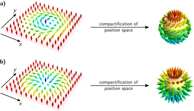
Figure 2.1.: Examples of two-dimensional skyrmions. In both cases, M ˆ winds once around the unit sphere and both skyrmions have winding number W = −1 and can be continuously deformed into each other. Arrows are spaced in arbitrary distances not related to the lattice distance and colored according to their z component. a) Bloch-type skyrmion, typically found in bulk chiral magnets such as MnSi. b) N´ eel-type skyrmion, typically found in thin films.

where the real fields fields φ

, α = 1, . . . , 4 have to satisfy the condition

φ

+ φ

+ φ

+ φ

= 1. (2.3) Thus, for a fixed time t, the combined field φ ≡ (φ

, φ

, φ

, φ

) defines a mapping from the compactified position space S

to S

. Generally, the space of mappings from S

to S

separates into topologically disconnected classes, which form the n

homotopy group of S

, or π

(S

) for short. In the present scenario we have n = m = 3 and since π

(S

) is always isomorphic to Z (for n ≥ 1) [16], the field configuration at any given time can be labeled by an integer winding number,

W = 1 2π

Z

d

r

φ

∂φ

∂r

∂φ

∂r

∂φ

∂r

(2.4) where

is the totally antisymmetric tensor. Time evolution, described on a classical level by the Euler-Lagrange equations of L, is continuous and therefore the winding number is a constant of motion.

The integer winding number counts the number of times that φ(r) covers S

when r

is varied over the whole space. A given field configuration with winding number W can

2.1. Skyrmions as topologically stable objects always be continuously deformed into a configuration of W “elementary” solitons that are located far away from each other. These elementary solitons are nowadays referred to as skrymions and their properties are similar to those of particles: skyrmions can move in space and they possess internal degrees of freedom in the sense that the field configuration can be deformed locally. However, continuous deformations cannot change the overall number of skyrmions since the winding number is a topological invariant.

Thus, we started with a theory, Eq. (2.1), that contained the pion fields as the only particle fields, and we identified the topologically stable excitations of the pion field as a new emergent type of particles. In contrast to the collective excitations discussed above, skyrmions are not a coherent superposition of local excitations since they are not linear.

Scaling a skyrmion solutions φ by a factor of 2 does not lead to a configuration with two skyrmions but instead would violate the normalization condition Eq. (2.3).

The concept of topological excitations as emergent particles is not limited to three dimensions and it turns out that two-dimensional skrmions naturally appear in magnetic systems. These magnetic skyrmions are the topic of this thesis. The magnetization M(r) in a magnetic material is a three-component vector field. Below the transition temperature, the magnitude |M| of the magnetization becomes finite. Fluctuations of the magnitude are energetically expensive, while long-wavelength fluctuations of the direction M ˆ := M/|M| are governed by the energy scale of crystal anisotropies, which is often much lower in bulk materials. It is therefore often a good approximation to assume a constant |M| and consider only the free energy as a function of M. Two kinds ˆ of two-dimensional skyrmions are depicted in Figure 2.1. Bloch-type skyrmions where M ˆ winds like a screw on paths through the skyrmion center are typically found in bulk chiral magnets such as MnSi (Figure 2.1a). N´ eel-type skyrmions are often realized in thin films where inversion symmetry is broken by the existence of a substrate on only one side of the film (Figure 2.1b). Far away from the skyrmion, the magnetization is constant and we can again compactify position space to the sphere S

. The map M ˆ : S

→ S

has an integer winding number, which can be calculated from

W = 1

4π M ˆ · ∂ M ˆ

∂x × ∂ M ˆ

∂y

!

. (2.5)

The winding number counts the number of times that the unit sphere S

is covered when r varies over the whole plane, as depicted in the right part of the Figure. One obtains the value of W = −1 for both configurations in Figure 2.1. The configurations are therefore sometimes called anti-skyrmions. Note, however, that the sign of W depends on the way in which the order parameter space S

is embedded in R

. If we had looked at the two planes in Figure 2.1 from below, we would have obtained W = 1.

From a mathematical point of view, the winding number cannot be changed by con-

tinuous deformations of the magnetization texture. However, the topological protection

only holds if the order parameter is always well-defined and the magnetization never

vanishes. In real magnetic systems, the topological invariance of the winding number

translates into an energy scale for a barrier that has to be overcome in order to change

the winding number.

0.03 0.08 0.21 0.55 1.47 3.87 10.2 27.1 71.5 189 500

Counts/Std.mon.

0.08

0

-0.08

qy(Å-1)

0.08 0

-0.08

q_x(Å^-1)

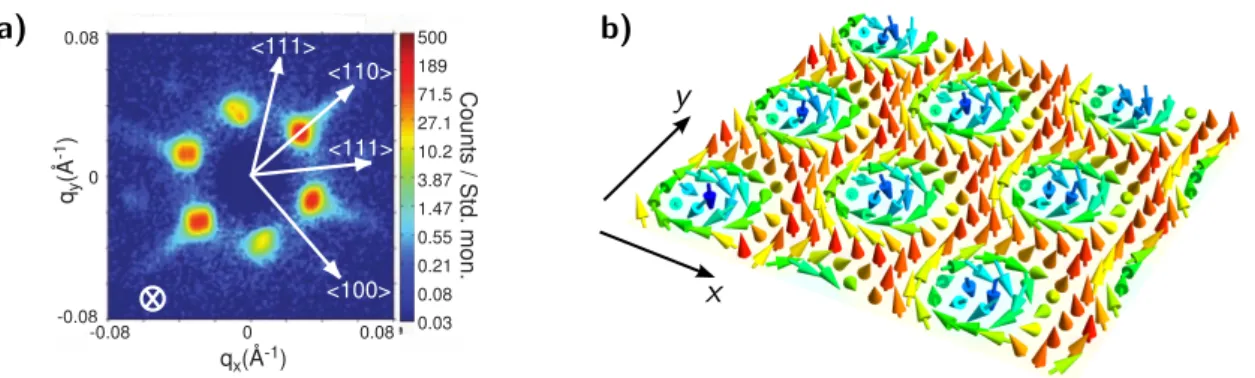
Figure 2.2.: Skyrmion lattice phase in MnSi; a) Typical intensity pattern in small angular neutron scattering experiments in the skyrmion lattice phase. Figure taken from Ref. [9]. The magnetic field points in the direction of the beam. White arrows indicate symmetry axes of the crystal. b) The superposition of three helices with coplanar wave vectors, an angle of 120

between each pair of wave vectors, and appropriate relative phases is a skyrmion lattice.

2.2. Skyrmion lattice phase in chiral magnets

In 1988, Bogdanov and Yablonskii [17] predicted that thermodynamically stable vortices, similar vortex lattices in super conductors, exist in magnetic materials with an easy- axis magnetic anisotropy. Their analysis was based on a mean-field calculation for a model with inversion-symmetric exchange interaction. In a later study by Bogdanov and Hubert [18], an exchange interaction with chiral asymmetry was considered in a similar model. The mean-field theory predicted the existence of a meta-stable hexagonal lattice of vortices. It is now known that, in the presence of a small external magnetic field, a lattice of skyrmions is stabilized by thermodynamic fluctuations in bulk magnetic materials with chiral asymmetry [9].

The first experimental discovery of a skyrmion lattice in magnetic materials was re-

ported in 2009 by M¨ uhlbauer and collaborators [9]. They examined a bulk sample

of MnSi in the ordered phase close to the transition temperature using small angular

neutron scattering (SANS). MnSi is a magnetic material with a transition temperature

around 29.5 K whose crystal structure has no inversion symmetry. A small external

magnetic field was applied parallel to the neutron beam. The recorded scattering im-

age shows a pattern of six Brag peaks symmetrically aligned around the center (Figure

2.2a). Since neutrons couple primarily to the magnetization, the scattering intensity is

proportional to the spin-spin correlation function in momentum space. Each pair of op-

posite brag peaks at wave-vectors q and −q corresponds to a helical spin configuration

in position space with wavelength 2π/|q| along the direction of q. If the neutron beam

is perpendicular to the magnetic field, only two Bragg peaks are observed, suggesting

that the three Helices lie in the same plane perpendicular to the magnetic field. The

superposition of three helices with 120

degree angle between each other results in a tri-

angular lattice of skyrmions for appropriate relative phases between the helices (Figure

2.2. Skyrmion lattice phase in chiral magnets 2.2b). The figure shows a cut through the system perpendicular to the applied magnetic field. The magnetization texture is translationally invariant in the direction along the magnetic field. It was confirmed by theoretical calculations that the skyrmion lattice is indeed the thermodynamically stable configuration.

In addition to SANS measurements, the existence of a skyrmion lattice phase in mag- netic materials without inversion symmetry has now been confirmed with a number of complementary methods. These scattering experiments were later supported by observa- tions of skyrmion lattices in real space using Lorentz Transmission Electron Microscopy for thin films [19], as well as magnetic force microscopy on the surface of bulk sam- ples [20]. In addition to these direct observations, the phase boundaries to the skyrmion lattice can also be inferred from electron transport experiments. Here, the existence of a skyrmion lattice leads to a strong additional contribution to the Hall resistivity [21, 22].

We provide a more detailed discussion of the so-called topological Hall effect in Chapter 7.

The skyrmion lattice phase is not limited to MnSi and it has been observed in a variety of systems. The doped semiconductor Fe

Co

Si was studied in [19, 23]. In thin films of FeGe [24], a skyrmion lattice phase was reported to exist up to approximately 260 K.

A strategy to engineer thin-film structures that can host skyrmions at room temperature has been proposed in Ref. [25] and single skyrmions at room temperature have recently been observed by Boulle and collaborators [26]. The discovery of a skyrmion lattice in the insulating multiferroic compound Cu

OSeO

[27] promises new possibilities to manipulate skyrmions via electric fields without resistive losses. All these systems have in common that the atomic structure has no inversion center. In thin films, inversion symmetry is broken due to the presence of a substrate on one side of the film. Bulk materials in which a skyrmion lattice phase has been observed all have a crystal structure whose space group has no inversion center, usually the P2

3 space group. Magnetic materials without inversion center are commonly referred to as chiral magnets. Each chiral magnet comes in two variants, a left-handed and a right-handed one, which are related to each other by space inversion. Due to the absence of inversion symmetry, the free energy functional F [M] contains non-inversion symmetric terms. In the Ginzburg- Landau theory of spontaneous symmetry breaking, one obtains F [M] by expanding in gradients of M and retaining all terms allowed by symmetry. Following the notation in [9], the free energy is given by

F [M] = Z

d

r [r

M

+ J (∂

M

)(∂

M

) + 2DM · (∇ × M) + U (M

)

− B · M]. (2.6)

Here, r

= 0 marks the transition from the unordered to the ordered state on a mean-

field level, D is the strength of the so-called Dzyaloshinskii-Moriya (DM) interaction, see

below, J is the ferromagnetic exchange coupling, U > 0 is needed so that the free energy

is bounded from below and B is the external magnetic field. The term proportional

to D is odd under space inversion and therefore only allowed in chiral magnets. Its

sign depends on the chirality of the crystal structure and it describes an anisotropic

exchange interaction derived by Dzyaloshinksii and Moriya [28,29]. The form of the DM

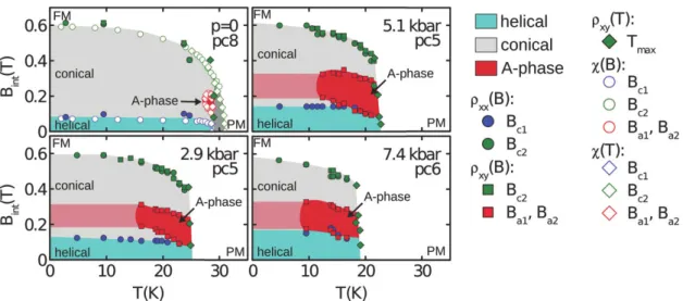
Figure 2.3.: Phase diagrams of MnSi at four different pressures from ambient pressure to 7.4 kbar. Figure taken from Ref. [30]. The skyrmion phase is labeled as

“A-phase” for historical reasons. Phase boundaries are inferred from mea- surements of magnetoresistance (ρ

(B)), Hall effect (ρ

(B) and ρ

(T)), and magnetic susceptibility (χ(B) and χ(T )).

interaction with a scalar prefactor D in Eq. (2.6) is applicable to materials with cubic symmetries, as are all bulk materials mentioned above.

Three energy scales govern the physics of chiral magnets [9]. On the largest energy scale, the exchange interaction J > 0 penalizes gradients of the magnetization. On an intermediate scale, the DM interaction D favors maximally twisted spin structures. It is typically smaller than the exchange interaction since it is mediated by spin-orbit inter- action, which is a relativistic effect. The competition between ferromagnetic exchange and DM interaction leads to helical structures with a wave vector of q = D/J ∼ λ

/a where λ

1 is the spin-orbit coupling strength and a is the lattice constant. On the lowest energy scale, crystal anisotropies, of higher order in λ

, pin the orientation of helices along symmetry directions of the crystal for small external magnetic fields.

Phase diagram of MnSi. In Figure 2.3, we show the phase diagram of MnSi at four

different pressures ranging from ambient pressure to 7.4 kbar. The figure is taken from

Ref. [30]. The diagrams combine data from measurements of the Hall resistivity, magne-

toresistance, and magnetic susceptibility, as indicated by the key. The general structure

of the phase diagram is archetypal for all bulk chiral magnets. In thin films with magnetic

field perpendicular to the sample, the skyrmion lattice phase typically extends down to

lower temperatures because the conical phase cannot exist for geometrical reasons, see

below. The following phases are indicated: At high temperatures, the system is in the

unordered paramagnetic state (PM). At low external magnetic fields, the system orders

in a helical state below the transition temperature. In this phase, the magnetization is

2.3. Recent trends described by

M(r) = M

cos(q · r) + M

sin(q · r) (2.7) where M

, M

, and q are all perpendicular on each other. The wavelength 2π/|q| of the helix in MnSi increases from 165 ˚ A near the transition temperature to 180 ˚ A for the lowest measured temperatures [31–33]. The direction of q is weakly pinned to along a [111]

direction due to crystal anisotropies. In the diagram for p = 0, a narrow fluctuation disordered phase is indicated in dark gray. In this regime, mean-field theory would already predict an ordered state, but helical fluctuations with wave vectors q uniformely distributed on a sphere in momentum space give rise to corrections to the mean-field behavior and drive the transition weakly first order [31].

As the magnetic field is increased in the ordered state, the magnetization changes into a conical state. In this state the magnetization is again described by Eq. (2.7), but the wave vector q aligns parallel to the magnetic field and M

and M

are no longer perpendicular on q but obtain a component in direction of the magnetic field. The nature of the transition from the helical to the conical state depends on the orientation of the crystal. In the general case it is a crossover but it may be a second-order transition if the magnetic field is applied along a [111] direction [34]. The angle between M and B decreases with increasing magnetic field up to the point that the two are parallel and the system is in the ferromagnetic state.

The skyrmion lattice phase, labeled “A-phase” in Figure 2.3 for historical reasons, forms a small pocket close to the transition temperature at a small external field B ∼ 0.2 T at ambient pressure. The phase extends to lower temperatures as pressure is increased [30]. Due to the topological protection of skyrmions, the skyrmion lattice remains metastable if the system is prepared in the in the skyrmion lattice phase close to the transition temperature and then the temperature is lowered (field cooling). This is indicated by the light red shaded area. If the system is cooled down at zero magnetic field (zero-field cooling) and then the magnetic field is turned on, the system prefers the conical phase. The fate of a metastable skyrmion lattice when the magnetic field is slowly reduced and then inverted has been studied in Refs. [20,35]. In a three-dimensional sample, this “unwinding” happens by a process in which two skyrmions first merge at a single point in space at which the magnetization vanishes. This singular point then runs through the system like a zipper. It turns out that the singular point is a source or sink of an emergent magnetic field, see Section 4.1.

2.3. Recent trends

A major reason for the recent interest in magnetic skyrmions lies in their prospect for future data storage devices. The topological protection of skyrmions makes them promising candidates for non-volatile storage devices, especially since single skyrmions in a ferromagnetic background can be realized in thin magnetic films [25,26]. In addition, it turns out that skyrmions can be very efficiently manipulated with electric currents [12].

This has two reasons. First, skyrmions couple to currents via a particular gyro-coupling,

which is related to the winding number of the skyrmion [11,36]. Second, unlike magnetic

bubbles, which have been known to exist in materials without chiral asymmetry since the 1970s [37], skyrmions in chiral magnets turn out to be rather rigid objects and forces on skyrmions couple predominantly to their translational mode rather than internal degrees of freedom [38]. In a numerical study, Fert and collaborators [39] proposed a setup by which a pattern of skyrmions that encodes a series of bits can be driven in a controlled way through a wire. Appropriately placed grooves in at the edge of the wire may help to control the placements of the skyrmions, or to nucleate skyrmions at sharp edges [40].

We study the dynamics of skyrmions with an emphasis on the influence of phase-space Berry phases in part III of this thesis (Chapters 9–11).

A different approach to the controlled manipulation of skyrmions is to selectedly create or destroy single skyrmions in a ferromagnetic background. In thin films, skyrmions can be created and destroyed by injecting a spin-polarized current from the magnetic tip of a scanning tunneling microscope [41,42]. Recent experiments by Hsu and collaborators [43]

indicate that it may be possible to generate and destroy skyrmions by electric fields

without a current. In part I of this thesis (Chapters 5–6), we show that skyrmions carry

an electric charge, which might provide an explanation for this mechanism.

3. Berry phases

In 1983, Michael Berry made the observation [1] that the wave function of a quantum- mechanical system picks up a geometric phase when the parameters in the Hamiltonian are changed slowly. A similar geometrical phase had already been identified by Pan- charatnam in 1956 in the context of classical optics [44]. This phase, today known as the Berry phase, influences the dynamics of the system and is ubiquitous in modern physics [2]. In this chapter, we discuss the mathematical and physical properties of Berry phases in a general setting. The application of these concepts onto chiral magnets is deferred to the next chapter.

This chapter is structured as follows. In Section 3.1, we discuss the general require- ments that lead to the appearance of Berry phases in a physical system. We derive a general expression for the Berry phase in section 3.2 and discuss the range of its ap- plicability in section 3.5. In Section 3.3, we discuss gauge invariance of Berry phase effects and give a geometric interpretation of the introduced quantities. In Section 3.4, we explicitly derive the Berry curvature for a spin in an external magnetic field. Finally, we discuss the validity of the adiabatic assumption in Section 3.5.

3.1. Origin of Berry phases in physical systems

If the Hamiltonian H(t) of a quantum system depends on time, the instantaneous eigen- states of H(t) are not stationary solutions of the time-dependent Schr¨ odinger equation.

However, if the time dependency of H(t) is sufficiently slow (to be quantified in sec- tion 3.5) and if the energy levels are non-degenerate for all times, then the adiabatic theorem [45, 46] states that a system that is prepared in the n

eigenstate of H(t

) at some initial time t

evolves in time by following the n

eigenstate of H(t) for t ≥ t

. Transitions into other eigenstates are exponentially suppressed as the time dependency of H(t) becomes slower.

While the adiabatic theorem guarantees that the system remains in the n

eigenstate

of H(t), it makes no statement about the phase factor e

that the wave function acquires

if the Hamiltonian returns to its original form, i.e. if H(t

) = H(t

) for some time

t

> t

. Berry’s observation [1] was that the phase picked up by a quantum system under

adiabatic time evolution can be understood as a sum of two contributions. First, the so-

called dynamical phase is the straight-forward generalization of the phase acquired by a

stationary state, and is given by the integral over time of the instantaneous eigenenergy

divided by ~. Second, there is an additional contribution, which Berry denoted as the

geometrical phase, and which is nowadays commonly referred to as the Berry phase. In

contrast to the dynamical phase, the Berry phase depends only on the instantaneous

eigenstates of H(t) and is insensitive to the eigenenergies.

The concept of Berry phases has been successfully applied in many branches of physics (see, e.g., Refs. [2–4]). This popularity may be explained by a combination of properties of the Berry phase.

First, Berry phases are physically measurable. Although the global phase factor of a wave function cannot be detected, Berry phases lead to interference when the adiabatic change from the initial Hamiltonian H(t

) to some final Hamiltonian H(t

) may be realized in more than one way. This is the generic situation if H(t) ≡ H(λ

(t), . . . , λ

(t)) is an effective Hamiltonian for the fast modes of a system where the dynamics of some slow degrees of freedom λ

(t), i = 1, . . . , N, is neglected (see below).

In this case, the parameters λ

may evolve from some initial to some final set of values on different trajectories. The different Berry phases picked up on these trajectories lead to interference and, ultimately, influence the effective equations of motion for the slow modes λ

once their dynamics is reintroduced into the theory. As interference experiments can only measure phase differences, only differences between Berry phases are physical. In contrast, the Berry phase along a single (not closed) trajectory in parameter space depends on the choice of basis at the initial and final time. We will come back to this gauge degree of freedom in section 3.3.

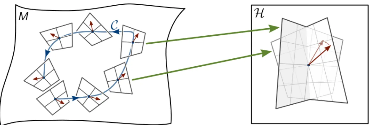
Second, there exists an intuitive geometric interpretation of Berry phases, allowing for the application of powerful tools from differential geometry and from topology to quantum mechanical problems. The Berry phase along an infinitesimal path in parame- ter space {λ

}

may be interpreted as an affine connection, so that adiabatic time evolution becomes equivalent to parallel transport of the wave function along a path in parameter space [47]. While an affine connection depends on the local coordinate sys- tem (i.e., the choice of gauge), it gives rise to a gauge-independent quantity called the (Riemann) curvature tensor. In absence of degeneracies, the so-called Berry curvature is simply the Berry phase along an infinitesimal loop in parameter space. For a compact parameter space, the total curvature is a topological invariant, i.e. it only depends on global properties of the connection and is insensitive to local perturbations. This opens up powerful tools from the field of topology that can be used to explain physical phe- nomena and classify states of mater. For example, the quantization of the transverse conductivity in the quantum anomalous Hall effect [48] is a direct consequence of the quantization of the total Berry curvature in the Brillouin zone [8, 49].

Finally, Berry phases are ubiquitous in nature, since they appear whenever a quantum- mechanical system exhibits a clear separation of time scales. The time dependency of the Hamiltonian H(t) may either be explicit due to an externally applied slowly time- dependent perturbation; or it may be an implicit time-dependency of an effective Hamil- tonian for the fast degrees of freedom of a system whose constituents are governed by dynamics on clearly separated energy scales. Both scenarios are particularly common in condensed matter physics. Many experiments on solids, for example, measure macro- scopic quantities such as thermal properties or transport coefficients in a macroscopic sample, while a microscopic description of the constituents is characterized by a much

1For an argumentation that focuses more on the mathematical properties of Berry phases, see also [2]

and references therein.

3.1. Origin of Berry phases in physical systems smaller length scale (the lattice constant) and therefore much larger momenta and ener- gies. In addition, the characteristic energy scales for the constituents themselves span a wide range from the Debye frequency for phonons ( ~ ω

∼ 10 . . . 100 meV) to the band width of the electronic system (∼ eV).

Let us illustrate the link between the separation of time scales and the appearance of a geometric phase by means of a classical analog. We consider a Foucault pendulum. Here, the two time scales are the short period τ of the oscillating pendulum and the long period T of the earth’s rotation, which is a sidereal day (about four minutes short of a solar day).

Except at the reversal points, the angular momentum L of the pendulum is primarily governed by the fast mode and therefore horizontally aligned. The gravitational force F

on the mass of the pendulum is downwards by definition, and therefore the torque L ˙ = r × F

is also in the horizontal plane (r points from the suspension point of the pendulum to the oscillating mass). However, the notion of “horizontal” changes slowly over time due to the rotation of the earth, and the angular momentum of the pendulum has to follow the horizontal plane. Microscopically, this process is mediated by a tiny torque due to the Coriolis force. It is rather cumbersome to solve the resulting equations of motion explicitly, since the Coriolis force depends on the velocity of the pendulum, which oscillates on the short time scale. To leading order in τ /T , it turns out that the direction of L follows the path that is defined by the smallest possible change consistent with the condition of staying in the horizontal plane [50]. The trajectory of the direction of L is therefore only governed by geometric aspects, namely the curvature of the surface of the earth and the latitude φ at which the experiment is carried out. It turns out that the direction of L, and therefore the orientation of the pendulum, rotates by an angle of 2π sin(φ) per sidereal day, where φ is measured from the equator. This is precisely 2π minus the solid angle enclosed by the location of the experiment on the surface of the earth as it rotates around the earth’s axis during one day.

In the classical example of the Foucault pendulum, the rotation angle can be observed directly. Quantum-mechanical phases, on the other hand, can only be observed if two wave functions interfere with each other. Therefore, Berry phases only play a role if the process that happens on the long time scale T is itself dynamic rather than externally imposed. Bloch electrons in an external electric field E are a prime example of such a separation of time scales. We may treat the electric field either in the current gauge, E = −∂A/∂t, where A(t) is the vector potential. This treatment is an example of an explicitly time-dependent Hamiltonian. The vector potential enters the Hamiltonian via the minimal coupling p = π + eA(t), where p and π are the kinetic and canonical momentum of the electrons with charge −e, respectively. A natural time scale τ

associated with the external perturbation is given by the time in which the difference p − π = eA(t) traverses the Brillouin zone once. This leads to the estimate

~ a = e

∂A

∂t

τ

= e|E|τ

(3.1) where a ∼ ˚ A is the lattice constant. Thus, the characteristic energy ~ /τ

= ea|E|

of the external perturbation is the energy an electron gains when it travels one lattice

constant in the direction of the electric field. Even for very large electric fields, this value is much smaller than the band separation ∆E ∼ eV, which is the characteristic energy scale for electrons in the unperturbed system.

Alternatively, we could have described the external electric field in the potential gauge, E = −∇φ, where φ(r) is the electric potential. In this treatment, the Hamiltonian is formally independent of time, but it gives rise to dynamics on two different time scales.

The fast dynamics are described by the unperturbed Hamiltonian, whose eigenstates Ψ

(r) = e

u

(r) are labeled by a band index n and a lattice momentum ~ k and may be written as a product of a plane wave and a Bloch function u

(r). The latter has the same periodicity as the atomic lattice. The electric potential φ(r) breaks the discrete translational symmetry and therefore the wave functions Ψ

(r) are no longer stationary. If we require again that ea|E| ∆E, then matrix elements hΨ

|φ(r)|Ψ

i between two different bands n 6= n

are small since the Bloch functions oscillate on a much shorter length scale than the electric potential. Thus, inter-band transitions are suppressed. On the other hand, intra-band matrix elements hΨ

|φ(r)|Ψ

i between to close-by wave vectors k and k

are not suppressed (in a finite system) since the quickly oscillating factor u

(r)u

(r) in the integrand is almost everywhere positive for k

≈ k. To a good approximation, the effect of intra-band transitions can be described by a slow time evolution of the lattice wave vector k(t). The remaining (fast) degrees of freedom are captured by the Bloch function, which follows, in this approximation, adiabatically the trajectory of k(t) in the Brillouin zone. Thus, the electron dynamics in the presence of an external electric field is described by a time-dependent effective Hamiltonian H

(t) = H(k(t)), where H(k) := e

He

is the band Hamiltonian.

We will see in section 5.1, that the time dependency of H

leads to Berry phases, which influence the trajectory of k(t).

3.2. Geometrical phase in a time-dependent system

In this section, we derive a general equation for the geometric phase picked up by a wave function under adiabatic time evolution due to a slowly time-dependent Hamiltonian.

We follow the original derivation by Berry in [1].

We consider a quantum mechanical system whose Hamiltonian H(λ(t)) depends on some time-dependent parameters λ(t) ≡ (λ

(t), . . . , λ

(t)) ∈ M , where the parameter space M is a real manifold. As discussed in the introduction to this chapter, the param- eters λ(t) may either be externally applied time-dependent fields, or H(λ(t)) may be the effective Hamiltonian of a more complicated system that contains some slow modes {λ

(t)}

, whose dynamics is neglected for the moment. For example, if λ

≡ k

are the lattice wave vectors in an N -dimensional crystal, then M is the Brillouin zone, which is an N -torus. For fixed λ, the Hamiltonian has eigenenergies E

(λ) and corresponding normalized eigenstates |Φ

(λ)i, defined by

H(λ)|Φ

(λ)i = E

(λ)|Φ

(λ)i, hΦ

(λ)|Φ

(λ)i = 1. (3.2)

We refer to E

(λ) and |Φ

(λ)i as the instantaneous eigenenergies and eigenstates,

3.2. Geometrical phase in a time-dependent system respectively, and assume that the instantaneous eigenenergies are discrete and non- degenerate for all times. Note that Eq. (3.2) defines each instantaneous eigenstate only up to a global phase. We require that these phases are chosen such that the maps λ 7→ |Φ

(λ)i are differentiable. It is important to keep in mind that such a differen- tiable choice of instantaneous eigenstates is not always possible on the whole parameter space M (see example at the end of section 3.3). For the present purpose, however, we only require that the maps are differentiable on an open subset of M that contains the trajectory λ(t) during the (finite) time interval of interest, which is always possible.

Suppose that at some initial time t

, the wave function |Ψi of the system is prepared in the n

instantaneous eigenstate, |Ψ(t

)i ∝ |Φ

(λ(t

))i. Time evolution is described by the Schr¨ odinger equation,

i~ ∂

∂t |Ψ(t)i = H(λ(t)) |Ψ(t)i. (3.3) If λ(t) varies sufficiently slowly (see section 3.5), then |Ψ(t)i follows adiabatically the n

instantaneous eigenstate. We thus make the ansatz

|Ψ(t)i = e

|Φ

(λ(t))i (3.4) where ϕ(t) ∈ R is a yet to be determined phase. Combining Eqs. (3.2), (3.3) and (3.4) and projecting onto hΦ

(λ(t))| leads to

∂ϕ(t)

∂t = − E

(λ(t))

~ +

N

X

i=1

∂λ

∂t A

(λ(t)) (3.5)

where

A

(λ) = ihΦ

(λ)| ∂

∂λ

|Φ

(λ)i (3.6)

is the i

component of the Berry connection of the n

energy level, which is real due to the normalization hΦ

(λ)|Φ

(λ)i = 1. By integrating Eq. (3.5) we find for the phase picked up by a quantum state subject to adiabatic time evolution from t

to t

,

∆ϕ

≡ ϕ(t

) − ϕ(t

) = − 1

~ Z

t0

E

(λ(t)) dt + ∆ϕ

(3.7) with

∆ϕ

= Z

C

dλ · A

(3.8)

where C := λ([t

, t

]) ⊂ M is the path in parameter space on which the parameters are varied and the notation dλ ·A

denotes the scalar product (i.e., sum over all components i = 1, . . . , N).

Eq. (3.7) describes the phase under adiabatic time evolution as a sum of two contri-

butions. The term involving the integral over time is called the dynamical phase. It

generalizes the phase factor e

of a stationary state in a time-independent system

to the situation where the eigenenergy E

depends slowly on time. The second term,

∆ϕ

, is a correction to this na¨ıve generalization. ∆ϕ

is the Berry phase for an adiabatic change of parameters along the path C. Note that the Berry phase depends only on the (directed) contour C on which the parameters λ are varied, and is independent of the velocity with which λ(t) changes as a function of time (provided that the change remains adiabatic). For this reason, the Berry phase is sometimes called a geometrical phase.

Note also that the Berry phase along the reversed path ¯ C is given by ∆ϕ

= −∆ϕ

.

3.3. Gauge invariant formulation and geometric interpretation of Berry phases

The Berry connection, Eq. (3.6), cannot be a physically measurable quantity since it depends on the choice of phases for the instantaneous eigenstates |Φ

(λ)i. The freedom to choose an arbitrary phase factor for each instantaneous eigenstate at all λ ∈ M constitutes a U (1) gauge degree of freedom for the solutions of Eq. (3.2). For a given choice of phases, we may define an alternative set of instantaneous eigenstates via the gauge transformation

|Φ

(λ)i 7−→ e

|Φ

(λ)i (3.9) where α

: M → R are arbitrary differentiable functions. The Berry connection, Eq. (3.6), changes under the gauge transformation,

A

(λ) 7−→ A

(λ) − ∂α

(λ)

∂λ

. (3.10)

Therefore, the Berry phase, Eq. (3.8), is also gauge dependent,

∆ϕ

7−→ ∆ϕ

− Z

C

dλ · ∂α

(λ)

∂λ = ∆ϕ

− α

(λ(t

)) + α

(λ(t

)). (3.11) Eq. (3.11) simply reflects the fact that the gauge transformation, Eq. (3.9), changes the reference states to which the phases at times t

and t

are measured.

Berry curvature. When one derives semiclassical theories that include Berry phase

effects, it is of advantage to formulate the semiclassical theory only in terms of gauge-

invariant quantities. The gauge dependency of results obtained from a semiclassical

theory can sometimes be quite subtle [51] if the semiclassical theory does not exclude

gauge-dependent quantities right away. An important gauge-invariant quantity is given

by the Berry phase along a loop in parameter space. If λ(t

) = λ(t

), the last two terms

on the right-hand side of Eq. (3.11) cancel and ∆ϕ

is gauge invariant. In the same way,

the difference ∆ϕ

− ∆ϕ

between the Berry phases along two different paths C

and

C

with common start and end points is gauge invariant, since it is equal to the Berry

phase ∆ϕ

picked up along the loop C that results from attaching the reverse of C

to

the end of the path C

(Figure 3.1).

3.3. Gauge invariant formulation and geometric interpretation of Berry phases

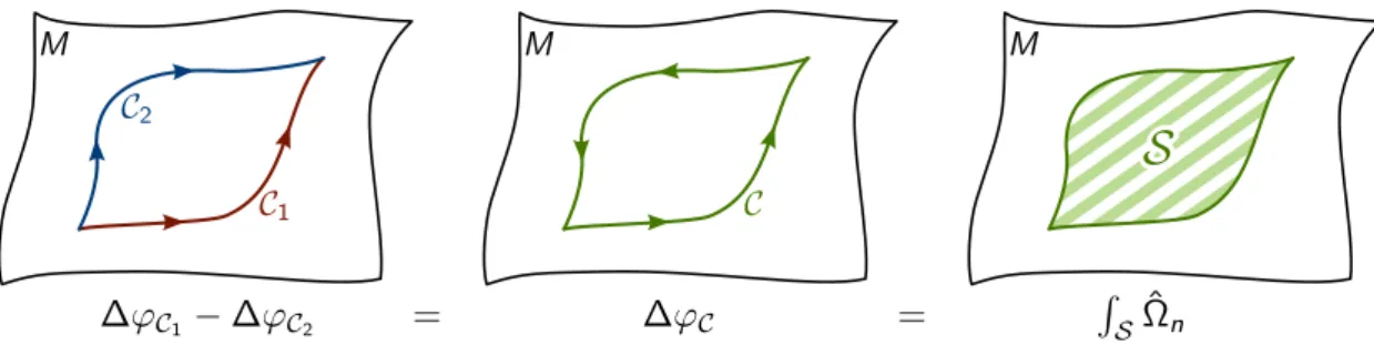
Figure 3.1.: The difference ∆ϕ

− ∆ϕ

between the Berry phases along two paths C

and C

with common start and end points is gauge invariant since it is equal to the Berry phase ∆ϕ

along a loop C resulting from attaching the reverse of C

to the end of C

. If C is contractible, then ∆ϕ

can be calculated by integrating the Berry curvature Ω

over any surface S with ∂S = C, Eq. (3.12).

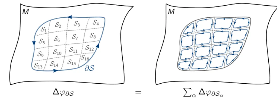
While the Berry phase along a loop C ⊂ M is gauge-invariant, it is difficult to include in a semiclassical theory due to its non-locality. This obstacle can be overcome if C can be contracted to a point, in which case the Berry phase along C can be expressed in terms of a local, gauge-invariant quantity known as Berry curvature. A contractible loop C can be expressed as the boundary ∂S of some surface S ⊂ M . According to Stokes’

theorem, one has for the Berry phase along C,

∆ϕ

= Z

∂S

dλ · A

= 1

~ Z

S

Ω

(3.12)

where the two-form Ω

= 1

2

N

X

i,j=1

Ω

(λ) dλ

∧ dλ

with Ω

(λ) = ∂A

∂λ

− ∂A

∂λ

(3.13) is the Berry curvature in the energy level n, which is invariant under the gauge transfor- mation Eq. (3.10) (“∧” denotes the totally anti-symmetric wedge product). The com- ponents Ω

= −Ω

of the Berry curvature form a skew symmetric tensor, usually referred to as the Berry curvature tensor, and satisfy the Jacobi identity

∂Ω

∂λ

+ ∂Ω

∂λ

+ ∂Ω

∂λ

= 0 (3.14)

which can be easily checked.

Intuitively, one can understand Eq. (3.12) by dividing the surface S into infinitely many infinitesimally small pairwise disjoint surfaces S

such that S = S

α

S

(Figure

3.2 left). The (directed) path C = ∂S is the sum over all directed paths ∂S

around the

tiles S

, as the paths along the boundaries between two neighboring tiles S

and S

cancel due to opposite orientation (Figure 3.2 right). Thus, the Berry phase around the

Figure 3.2.: The Berry curvature along the boundary ∂S of a surface S may be ex- pressed by dividing S into small tiles S

(left), and summing over the Berry curvatures along the boundary of each tile (right). The paths along a shared boundary cancel due to opposite orientation.

whole surface S is equal to the sum of the Berry phases around each tile S

. It is easy to see that, in the limit of infinitesimally small tiles, the Berry phase around a tile S

that lies in the plane spanned by λ

and λ

is given by the area of the tile multiplied by Ω

.

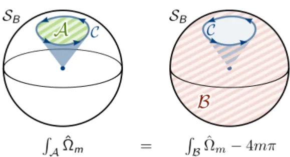
Eq. (3.12) expresses the Berry phase along a loop C in terms of the local, gauge invariant Berry curvature. The relation holds for any loop C that can be contracted to a point (Figure 3.3 left). If C is not contractible (e.g., if M is a torus and C winds around one of its circles, see Figure 3.3 right), then there is no surface S with the property C = ∂S. Consequently, the Berry phase along a non-contractible loop cannot be expressed in terms of the Berry curvature Ω

, and one has to resort to Eq. (3.8) to calculate ∆ϕ

from the Berry connection A

. This scenario is similar to the Aharonov- Bohm effect [52]. In momentum space, non-contractible trajectories exist since the Brillouin zone is a torus. The Berry-phase around the Brillouin zone of a one-dimensional crystal is known as the Zak phase [53]. It was recently observed in an ultracold gas of

87

Rb atoms [54].

Numerical evaluation of the Berry curvature. Combining Eqs. (3.6) and (3.13), the components of the Berry curvature are given by

Ω

(λ) = i

∂hΦ

|

∂λ

∂|Φ

i

∂λ

− ∂hΦ

|

∂λ

∂|Φ

i

∂λ

= −2 Im

∂hΦ

|

∂λ

∂|Φ

i

∂λ

(3.15)

where we refrained from writing out the parameter λ of the instantaneous eigenvectors

in order to improve readability. Eq. (3.15) can be used to calculate the Berry curvature

for a given Hamiltonian H(λ) if the instantaneous eigenvectors |Φ

(λ)i are differentiable

in the chosen gauge. However, this is not always the case. In a numeric calculation,

one may be tempted to rasterize the parameter space and find the instantaneous eigen-

vectors for all points λ on a grid with finite spacing, replacing derivatives by difference

3.3. Gauge invariant formulation and geometric interpretation of Berry phases

Figure 3.3.: Left: If the parameter space M is simply connected (e.g., M = S

is the surface of a sphere), then every loop C ⊂ M can be smoothly contracted to a point. The surface S that is covered by the loop during its contraction to a point has the property ∂S = C, such that Eq. (3.12) applies. Right:

Example of a non-contractible loop C on a torus M = S

× S

, which is not simply connected. Here, Eq. (3.12) cannot be applied to calculate the Berry curvature along the loop.

quotients. Since the numerical diagonalization routine may produce eigenvectors with arbitrary phases, the difference quotients can become arbitrarily large. Even in ana- lytical calculations, a choice of gauge such that |Φ

(λ)i is differentiable on the whole parameter space M does not always exist.

For a finite-dimensional Hilbert space, a numerically more stable expression for Ω

can be obtained by using the relation

(E

− E

) hΦ

| ∂|Φ

i

∂λ

= δ

∂E

∂λ

−

Φ

∂H

∂λ

Φ

, (3.16)

which can be found by carrying out the derivatives on both sides of the equation hΦ

| ∂

∂λ

(H|Φ

i) = hΦ

| ∂

∂λ

(E

|Φ

i). (3.17)

Inserting an identity operator 1 = P

m

|Φ

ihΦ

| in-between the two derivatives on the right-hand side of Eq. (3.15) and using Eq. (3.16) leads to

Ω

(λ) = −2 X

m6=n

Im

"

Φ

∂λi

Φ

Φ

∂λj

Φ

(E

− E

)

#

, (3.18)

where the term with m = n drops out of the sum since it is real. Eq. (3.18) suggests to

interpret the Berry curvature as consequence of virtual transitions into different energy

levels m. Even though we restrict the wave function to a single energy level n by

assuming adiabatic time evolution, the presence of other energy levels m 6= n is essential

for a non-vanishing Berry curvature. Generically, we expect a large Berry curvature if

off-diagonal elements of the Hamiltonian in the basis of instantaneous eigenstates change

rapidly and if energy levels come close to each other, e.g. at an avoided crossing of energy

levels (see example in section 4.3).

Figure 3.4.: Left: The complex line bundle B

, Eq. (3.19), is defined by attaching a one-dimensional complex vector space, here depicted as two-dimensional (real) planes, to each point λ ∈ M . A reference state |ψ(t)i (red arrows) changes its direction under parallel transport along a loop C ⊂ M due to the holonomy of the parallel transport. Right: B

admits for a natural parallel transport because all attached complex vector spaces are subspaces of the same Hilbert space H. The natural parallel transport is defined by minimizing the distance (dashed red line) between |ψ(t)i and |ψ(t + dt)i, while keeping the norm of the state constant (Eq. (3.20)).

Geometric interpretation. The Berry phase along a loop C admits for a simple geo- metric interpretation. This has been pointed out in an article by Simon [47], which we summarize in the following. If we prepare the wave function |Ψi of a system at time t

in the n

instantaneous eigenstate, |Ψ(t

)i = |Φ

(λ(t

))i, then the adiabatic theorem restricts the space of accessible wave functions for all t ≥ t

to the n

eigenspace of H(λ(t)). This attaches (in absence of degeneracies) a one-dimensional complex vector space to each point λ ∈ M , thus defining the complex line bundle (c.f., Figure 3.4 left) B

:= {(λ, |φi) : λ ∈ M ∧ H(λ)|φi = E

(λ)|φi}. (3.19) In order to define a phase picked up by |Ψ(t)i as λ(t) varies over time, we have to compare the state |Ψ(t)i to some reference state that also lies in the n

eigenspace of H(λ(t)).

We cannot use the initial state |Ψ(t

)i as the reference state since the eigenspaces of H(λ) may depend on λ. In section 3.2, we used the state |Φ

(λ(t))i as a reference, but, as discussed above, |Φ

(λ(t))i is only defined up to an arbitrary phase, thus rendering the relative phase between |Φ

(λ(t))i and |Ψ(t)i gauge dependent. A gauge-independent reference state |ψ(t)i is defined by parallel transport of the initial state |Ψ(t

)i along the trajectory λ(t) in the line bundle B

(Figure 3.4 left). While many definitions of parallel transport are conceivable, B

admits for a natural definition of parallel transport [55]

as it is embedded in the product space M × H, where H is the Hilbert space. The natural parallel transport is defined by the property that it minimizes the rate of change

||∂|ψ(t)i/∂t|| under the boundary condition that |ψ(t)i is normalized and lies in the n