Vector Chiral Phases in Frustrated Systems
Inaugural-Dissertation zur
Erlangung des Doktorgrades
der Mathematisch-Naturwissenschaftlichen Fakultät der Universität zu Köln
vorgelegt von
Hannes Schenck aus Berlin-Wilmersdorf
Universität zu Köln 2015
Berichterstatter: Prof. Dr. Thomas Nattermann Prof. Dr. Joachim Krug
Tag der letzten mündlichen Prüfung: 23.06.2015
Diese Arbeit ist meinen ElternIngolf & Annettegewidmet
Zusammenfassung
Die vorliegende Dissertation setzt sich aus zwei verschiedenen Teilen zusammen. Der erste Teil der Arbeit befasst sich mit der Untersuchung von chiraler Ordnung und ihrem Ursprung in frustrierten Wechselwirkungen. Zunächst wird das Konzept von Phasenübergängen und deren Relation zu der dem System zugrunde liegenden Symmetrie beschrieben. Hier wird diskutiert wie die diskreteZ2-Symmetrie der Ising-Spins und die kontinuierliche SO(2)-Symmetrie der XY- Spins in zwei Dimensionen zu fundamental verschiedenen Phasenübergängen führen. Als nächstes werden verschiedene Formen von chiraler Ordnung diskutiert, sowie deren experimentelle Rea- lisierung. Chirale Ordnung bricht die diskrete Inversions-Symmetrie (Z2), die simultan mit der SO(2)-Symmetrie der XY-Spins auftreten kann. Eine zentrale Fragestellung der Arbeit ist, zu klären, wie die Phasenübergänge sich durch das Auftreten der zusätzlichen Symmetrien verän- dern. Als archetypisches Modell für das gleichzeitige Auftreten von diskreter und kontinuierlicher Symmetrie wird das sogenannte helikale XY-Modell untersucht. Das Modell selbst wird als Er- weiterung des klassischen XY-Modells eingeführt und ausführlich diskutiert. Es wird beschrieben, wie durch die Einführung einer frustrierten Wechselwirkung das System einen chiralen Grund- zustand ausbilden kann und welche verschiedenen Ansätze es gibt, die simultanen Symmetrien zu untersuchen. Zusätzlich wird eine mesoskopische Version des Modells abgeleitet.
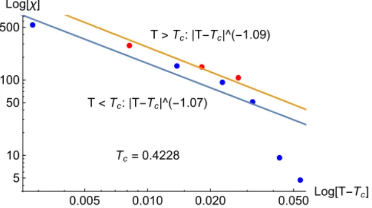
Zunächst wird der Phasenübergang der chiralen Ordnung diskutiert. Hier wird mittels des Va- riationsprinzips die kritische Temperatur für den Übergang gefunden sowie die Abhängigkeit der Temperatur vom Spiral-Winkel θ der Grundzustandsspirale. Anschließend wird der Effekt von chiraler Ordnung auf den Berezinskii-Kosterlitz-Thouless (BKT) Übergang der SO(2)-Symmetrie in dem Modell untersucht. Die für den BKT-Übergang verantwortlichen Vortizes werden auf klei- nen und großen Skalen diskutiert und die Energiekosten des Vortex-Kerns abgeschätzt. Mittels Renormierungsgruppen-Rechnung werden die Effekte der Vortizes auf den Phasenübergang un- tersucht und deren kritische Exponenten bestimmt. Anschließend wird die anomale Skalierungs- dimension des chiralen Übergangs bestimmt. Die Daten der numerischen Simulationen von Soro- kin et al. werden verwendet, um die kritischen Exponenten zu bestimmen und mit den errechne- ten Werten zu vergleichen. Das entstehende Phasendiagramm wird beschrieben sowie mögliche experimentelle Systeme und die Relation zu anderen theoretischen Arbeiten werden diskutiert.
Weiterführend wird näher auf den Zusammenhang zwischen chiraler Ordnung und Polari- sation in multiferroischen Systemen eingegangen. Verschiedene Mechanismen für die Kopplung von magnetischer und elektrischer Ordnung werden diskutiert und ausgehend von Symmetrie- Überlegungen wird das HXY-Modell um eine Wechselwirkung mit einem elektrischen Feld er- weitert. Diskutiert werden die Effekte der Polarisation auf die Domänenwände im System. Die resultierenden Sattelpunktsgleichungen werden näherungsweise gelöst und mit numerischen Re- sultaten verglichen. Des Weiteren wird die effektive Wechselwirkung zwischen den chiralen Domä- nenwände und den Domänenwänden in der Polarisation ermittelt und als gegenseitige Anziehung identifiziert.
Als konkretes Beispiel eines multiferroischen Materials wird das Material MnWO4 näher dis- kutiert. Hier koppelt chirale Ordnung an Polarisation gekennzeichnet durch einen magnetischen Phasenübergang, der mit dem Auftreten einer messbaren Polarisation einhergeht. Hier wurde in Zusammenarbeit mit der Arbeitsgruppe von Prof. J. Hemberger das kritische Verhalten an dem Phasenübergang untersucht. Zunächst werden die beobachteten Phasenübergänge in MnWO4
beschrieben und näher auf die Kristallsymmetrie eingegangen. Ausgehend von der von Tolédano bestimmten Ginzburg-Landau Freien Energie des Systems wird der Phasenübergang klassifiziert und das kritische dynamische Verhalten bestimmt. Die resultierenden Exponenten werden mit der experimentellen Arbeit der Arbeitsgruppe von Prof. J. Hemberger verglichen.
Im zweiten Teil der Arbeit wird das dynamische Verhalten von Vortizes in dünnen supra- leitenden Filmen untersucht. Zunächst wird ein historischer Überblick über die Entdeckung der Supraleitung gegeben und anschließend auf deren phänomenologische Beschreibung eingegangen.
Danach wird das Phänomen von supraleitenden Vortizes diskutiert und auf die Besonderheiten von Vortizes in dünnen Filmen eingegangen sowie deren Wechselwirkung mit einem extern an- gelegten Strom.
Zu Beginn wird der experimentelle Aufbau, der von der Arbeitsgruppe um Prof. E. Zeldov verwendet wird, beschrieben. Studiert werden hier Vortizes in dünnen supraleitenden Blei Filmen mittels SQUID-on-tip Raster-Mikroskopie. Bei angelegtem Strom können Vortizes in den Film eintreten indem sie eine Eintrittsbarriere überwinden. Diese Barrieren werden diskutiert und der Effekt auf die messbaren Strom-Spannungskurven wird bestimmt. Die Resultate werden mit den zur Verfügung stehenden experimentellen Werten verglichen.
Abschließend wird die Dynamik der Vortizes in den Filmen untersucht. Hier liegt das Augen- merk vor allem auf dem Effekt einer inhomogenen Stromdichte resultierend aus der experimentell angebrachten Verengung der dünnen Bleistreifen. Erklärt werden soll die Linienbildung der sich bewegenden Vortices, sowie das Entstehen von Verzweigungspunkten in diesen Linien. Es wer- den verschiedene Ansätze und effektive Modelle für die wechselwirkenden Vortizes diskutiert und deren Schwachstellen dargestellt.
Abstract
The present dissertation consists of two parts. The first part of this work deals with the study of chiral order that has its origin in frustrated interactions. First of all, the basic concept of phase transitions and their relation to the underlying symmetry will be described. Here we will discuss how the discreteZ2 symmetry of the Ising spins and the continuous SO(2) symmetry of the XY spins leads to fundamentally different phase transitions. Next, different forms of chiral order will be discussed, as well as their experimental realizations. Chiral order breaks the discrete inversion symmetry (Z2), which can appear simultaneously with the SO(2) symmetry of the XY spins. One of the central questions of this work is how the phase transitions are influenced by the additional symmetries. As an archetypical model for the simultaneous existence of both a discrete and continuous symmetry, the so-called helical XY model will be studied. The model itself will be introduced as an extension to the classical XY model and will be discussed in detail.
It will be described how the addition of a frustrated interaction leads to a chiral ground state and different approaches to dealing with these simultaneous symmetries are mentioned. Additionally, the mesoscopic version of the model will be derived.
We will start with the discussion of the chiral order phase transition. Using a variational method, the critical temperature of the transition and its dependance on the chiral pitch angle θwill be found. Afterwards, the effect of the chiral order on the Berezinskii–Kosterlitz–Thouless (BKT) transition of the SO(2) symmetry will be studied. The vortices responsible for the BKT transition will be discussed on short and large length scales and the energy cost of the vortex cores is estimated. Using the renormalization group technique, the effects of the vortices on the phase transition is studied and their critical exponents are estimated. Afterwards, the anomalous scaling dimension of the chiral transition is calculated. The data of the numerical simulations done by Sorokin et al. are used to determine the critical exponents and compare them to the analytic calculations. The resulting phase diagram for the HXY model is calculated and its relation to possible experimental systems and other theoretical works is discussed.
We will continue with a closer look at the relation between chiral order and polarization in multiferroic systems. Different mechanisms for the coupling of magnetic and electric order are discussed and, starting from a symmetry argument, the HXY model will extended by an interaction with the electric field. The effect of the polarization on the domain walls of the system will be studied. The resulting saddle-point equations will be solved perturbatively and are compared to numerical results. Additionally, an effective interaction between the chiral domain walls and the polarization walls will be derived and identified as an attractive interaction.
As a concrete example of a multiferroic material, the material MnWO4 will be studied. Here the chiral order couples to the polarization, as indicated by a magnetic phase transition with an accompanied onset of polarization. In collaboration with D. Niermann and the group of Prof. J. Hemberger, the critical behavior of the phase transition was studied. First the different phase transitions in MnWO4will be described and the crystal symmetry will be discussed. Start- ing from the Ginzburg–Landau free energy expansion done by Tolédano, the phase transitions will be classified and the critical dynamical behavior described. The resulting critical exponents are compared to the experimental work of the group of Prof. J. Hemberger.
In the second part of this work, the dynamical behavior of vortices in thin superconducting films is studied. First, a historical overview of the discovery of superconductivity is given,
followed by a discussion of it phenomenological description. Afterwards, the phenomenon of superconducting vortices is discussed and the special features of vortices in thin films and their interaction with an applied current are presented.
We start with a description of the experimental setup used in the group of Prof. E. Zeldov.
They study vortices in thin superconducting lead films with the SQUID-on-tip raster microscopy.
In the presence of an applied current, vortices can enter the thin strips by overcoming an entry barrier. These barriers are discussed and their effect on the measurable current–voltage curves is calculated. The results are compared to the available numerical data.
Finally, we study the dynamics of the vortices in thin films. The focus is on the effect of inhomogeneous current densities, a result from experimentally imposed constrictions in the thin films themselves. The task is to explain the formation of lines in the moving vortices and the existence of bifurcation points in said lines. Several approaches and effective models are used to study the interacting vortices, the results and shortcomings are discussed.
Contents
Contents vii
I Vector-Chirality and Spin-Liquid in Frustrated Systems 1
1 Introduction 3
1.1 Magnetic systems . . . . 4
1.2 Discrete and continuous symmetry in ferromagnets . . . . 6
1.3 Vector and scalar chiral order parameters . . . . 9
1.4 Physical realizations and experimental systems . . . . 11
1.5 Outline . . . . 13
2 The Model 15 2.1 The classical model . . . . 15
2.2 Quantum chain . . . . 20
2.3 Landau–Ginzburg–Wilson Hamiltonian . . . . 22
3 Chiral Transition 27 3.1 The variational approach . . . . 27
3.2 The solutions . . . . 31
3.3 Discussion . . . . 33
4 Renormalization Group 35 4.1 Vortices . . . . 35
4.2 Long–range interaction in Ising order parameter model . . . . 36
4.3 RG - small scales . . . . 37
4.4 RG - large scales . . . . 38
4.5 Anomalous dimension of chiral transition . . . . 42
4.6 Comparison to numerics . . . . 44
4.7 Phase diagram . . . . 45
4.8 Discussion . . . . 48
5 Multiferroics 53 5.1 Connection between chiral order and polarization . . . . 54
5.2 One–dimensional domain wall . . . . 56
5.3 Two–dimensional domain wall . . . . 65
5.4 Domain wall in “four-state” model . . . . 67
6 MnWO4 71 6.1 Material properties and observed phase transitions . . . . 71
6.2 Group theory construction of Ginzburg–Landau free energy . . . . 71
6.3 Classification of phase transitions and critical dynamics . . . . 74
6.4 Dynamical exponent atAF3 →AF2 . . . . 76
Contents Contents
6.5 Discussion . . . . 79
II Vortices in Supraconducting Thin Films 81 7 Introduction 83 8 Experimental Data 85 8.1 Experimental setup . . . . 85
8.2 Current–Voltage curves . . . . 88
8.3 Vortex dynamics . . . . 89
9 Superconductivity 91 9.1 Vortices . . . . 93
9.2 Vortex interaction . . . . 95
10 Current–Voltage Curves 97 10.1 Bardeen–Stephen flow . . . . 99
10.2 Surface barrier . . . . 101
10.3 Discussion . . . . 106
11 Vortex Dynamics 107 11.1 The Corbino disk setup . . . . 107
11.2 The current distribution in the Corbino disk . . . . 109
11.3 Non–local theory . . . . 110
11.4 Simple model for current–vortex interaction . . . . 114
11.5 Vortex–Current interaction - thin strip . . . . 117
11.6 Vortex–Current interaction - Corbino disk . . . . 120
11.7 Discussion . . . . 123
IIIAppendix 125 A Appendix: Model 127 A.1 XY quantum chain . . . . 127
A.2 Kolezhuk mapping . . . . 129
B Appendix: Renormalization Group 131 B.1 Vortex core energy integral . . . . 131
B.2 Fourier transform inx-direction . . . . 132
B.3 Calculating the constant pre-factorf(0) . . . . 133
B.4 Calculating thef(z→ ∞)limit . . . . 135
B.5 Solving the full Fourier transform . . . . 135
B.6 Solvingf(z)via ODE . . . . 136
B.7 Numerical calculation of the constantcx . . . . 137
B.8 Numerical data from Sorokin et al. . . . 138
C Appendix: Multiferroics 141 C.1 Integral Approximation . . . . 141
C.2 Python code for numerics . . . . 142
D Appendix: MnWO4 147
D.1 Different forms of order parameters . . . . 147
D.2 Transition atTN :temperature fluctuations inS˜1 . . . . 148
D.3 Transition atT2: FrozenS˜1 order parameter . . . . 150
E Appendix: Experiment 153 E.1 Material properties of lead . . . . 153
F Appendix: Vortex Dynamics 155 F.1 Detailed overview of current distribution . . . . 155
F.2 Derivation of main equations . . . . 159
F.3 Limiting cases and solutions to integral equations . . . . 162
F.4 Numerical approach . . . . 165
Bibliography 171
Part I
Vector-Chirality and Spin-Liquid in Frustrated Systems
1. Introduction
A material can be classified by its macroscopic properties such as density, volume, magnetization, resistivity and many more. In some cases, the macroscopic state can be changed by continuously varying an external parameter, such as the temperature, the applied magnetic field or the pres- sure. The system will undergo an abrupt change in one or more of its physical properties at a certain point in the parameter space of the external fields.
There are many examples of phase transitions in nature. To give a little idea of their diversity, we want to name just a few. The most commonly known example is the melting of a solid, as can be seen in water when melting an ice cube. Here the system changes from a ridged solid to a fluid.
Another example is the ferromagnet to paramagnet transition in magnetic materials such as iron (Fe). Here, the magnetization vanishes at the Curie temperature when heating up the material.
There are also structural phase transitions. In the material bariumtitanat (BaTiO3), varying the temperature results in a change of the crystal structure, [1]. This is is accompanied by a resulting electric dipole moment in each crystal cell and a global electric polarization. Another famous example are superconductors like lead (Pb). Here, the system switches from a finite resistance to superconductivity after the system is cooled below a critical temperature. A more detailed list and other examples can be found in standard literature such as [1, 2].
Essentially there are two ways in which a system can change from one phase to another. In the first case, the phases on either side of the transition line also coexist exactly at the transition, [3]. The phases still carry their distinct microscopical properties and are still distinguishable from each other despite the system being at phase transition. Away from the transition, the system will be in a unique phase that is continuously connected to the coexistence phase at the transition. One example for this type of transition is the melting of a solid in three dimensions, e.g. ice. In this case both the solid and liquid phase of water coexist. Additional heat is needed to drive the transition while there is no increase in the observed temperature of the mixture.
In a situation like this, we expect a discontinuity in one or more thermodynamic quantities, [3].
In the case of melting, this is reflected by a discontinuous change in entropy (first derivative of the free energy with respect to the temperature) of the system and the accompanied latent heat. Systems like this, where the phases coexist and the first derivative of the thermodynamic potential is discontinuous, are classified as first order or discontinuous transitions, [3]. In general they display a finite correlation length.
In the case of continuous phase transitions, the correlation length diverges at the critical point. Fluctuations are then correlated on all length scales throughout the whole system, forcing it into a unique state at the phase transition, [3]. In the case of a ferromagnet approaching the Curie temperature, the magnetization (first derivative of the free energy in respect to the applied field) continuously varies to zero. At the critical point the system is in a unique state without magnetization. As opposed to the first order transition, in this case we cannot identify coexisting regions with and without magnetization. However the susceptibility (second derivative of the free energy with respect to the applied field) diverges at the transition. This is an example of a second order or continuous phase transition. In general a phase transition in a system is connected to a singularity in the appropriate thermodynamic potential or its derivatives, [2].
In a lot of cases it is possible to identify a phase by its symmetry properties. A crystal for example, depending on its crystal structure, is invariant under certain discrete translations, dis- crete rotations around selected axis and points and other operations, all systematically classified
Chapter 1. Introduction 1.1. Magnetic systems
in the so called space groups, [1]. After melting, the system turns into a liquid that now exhibits continuous translation and rotation symmetry.
1.1 Magnetic systems
The microscopic origin of the magnetization is due to the spin of electrons in incomplete atomic shells, such as the f and d shell of transition metal atoms in iron, nickel, and cobalt, [4]. Each electron carries one Bohr magnetonµB of magnetic moment, [4]. In the ferromagnetic phase all these moments are aligned, resulting in a global magnetization of the material. This is due to an interaction between the magnetic moments that favors alignment in the ferromagnetic case and anti-alignment in the antiferromagnetic case.
Naively one might expect that the magnetic moments mainly interact via their magnetic dipoles. This is not the case. The magnetic interaction strength of two magnetic moments is of the order ofµ2B/d3∼1K, where we estimate the average distancedbetween the atoms with 1Å, [5]. Comparing this to the observed Curie temperature in e.g. Fe withTC∼1043K, we see that the interaction energy is lower by several orders of magnitudes. The dipole–dipole interaction is not strong enough to explain the high transition temperature.
Even without a direct force interaction between the spins, the quantum-mechanical symmetry constrain placed on the wave function will lead to an effective spin–spin interaction. To simplify the discussion, we will consider the case of two atoms with one free electron each. The complete wave function of the system is antisymmetric when switching the two electrons, due to their fermionic nature. Ignoring relativistic effects, the Schrödinger equation does not take the spin of the particles into account. The spin wave function and the orbital or position wave function are then independent of each other and the full wave function can be represented as the product of both, [6]. A symmetric orbital wave function then implies an anti-symmetric spin wave function and vice versa, in order to satisfy the anti-symmetry constraint of the full wave function. The system can now reduce the Coulomb repulsion between the two electrons by forming a symmetric spin state. In this case, the state of the two electrons is antisymmetric with a nodal point in between the two atoms. The probability of the electrons is now lowered in the exact region where their coulomb repulsion would be the strongest. On the other hand, the kinetic energy, i.e. gradient terms, associated with the anti-symmetric wave function is higher then for the symmetric one. Now depending on the ratio of repulsion energy versus kinetic energy, the system will favor the alignment or anti-alignment of the spins. In the case of iron the Coulomb repulsion term dominates, leading to the system favoring the alignment of the spins, i.e. ferromagnetic interaction. In the H2molecule, the actual overlap of the orbitals is small and the kinetic energy is the more important term, favoring anti-alignment of the spins. This is an easy example of anti-ferromagnetic interaction, [7, 8]. The interaction between the neighboring spinsSˆ1 and Sˆ2
can be simplified asJSˆ1Sˆ2, where all the microscopic details are absorbed in the constantJ. The sign ofJ determines the type of interaction and is ferromagnetic forJ <0and anti-ferromagnetic forJ >0 .
In materials like iron, the melting temperature TM is significantly higher than the Curie temperatureTC. In the case of iron we haveTM−TC ∼800K. When focusing on the magnetic transitions around TC, we are far away from the melting transition and can ignore structural changes in the lattice configuration. The system can then be treated as a collection of interacting spins on a fixed lattice as
H =X
ij
JijSˆiSˆj (1.1)
where the lattice information is contained in the coefficients Jij. Depending on the lattice
1.1. Magnetic systems Chapter 1. Introduction
anisotropies or crystal fields from neighboring atoms, the spins Sˆi can be restricted to a plane (XY spins) or even to just one axis (Ising spins). The complete structure of the phases and the physics of the phase transition is encoded in the configuration of the spins{Sˆi}on the sitesi.
Let us look at the example of a simple uniaxial ferromagnet, where crystal field anisotropies restrict the spin on each site to one axis, allowing only the alignment or anti-alignment with said axis, [3]. Ignoring quantum effects, we can replace the spin at each site by a classical variablesi
that can take on the values±1. In general, the phases can be classified by the n-point correlation function
Gn=hsisj. . . sk
| {z }
n
i. (1.2)
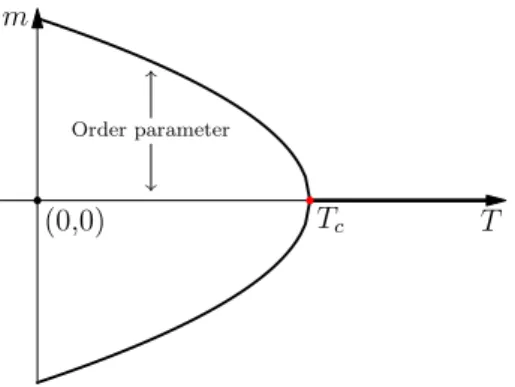
Here, the different phases can be classified by the one-point correlation function G1, i.e. the average magnetizationm=G1=hsii. In the ground state of the system all spins will be aligned and form the ferromagnetic phasem=±1. In the paramagnetic phase at high temperatures, the spins will fluctuate and, on average, not take on a specific value. In this case the magnetization vanishes and we have m= 0. The change of magnetization as a function of temperature m(T) without an applied field is shown in figure 1.1. We see that the magnetization continuously goes to zero and we are dealing with a second order or continuous phase transition at the Curie temperature.
T m
(0,0) Tc
Order parameter
Figure 1.1: Zero-field magnetization of a classical ferromagnet without an applied fieldH = 0.
We see a spontaneous magnetization ±m(T) below the critical temperature. The graphic is similar to the one used in [2].
On can also look at this phase transition in terms of a change in symmetry. Imagine the magnetic moment being caused by a circular current. Reversing time will now reverse the direction of the current and consequently flip the sign of the resulting magnetic moment. In mathematical language this means that the time reversal operatorTˆ :t7→ −t will flip the spin SˆiasTˆSˆiTˆ−1=−Sˆi. We can see that the simple magnetic Hamiltonian (1.1) is invariant under time reversal. The magnetization hSˆii, however, is not. In the present case of classical discrete spinssithis means thatm(T)7→ −m(T)under time reversal, making the ground statem(T)6= 0 doubly degenerate. The paramagnetic casem(T) = 0, the state of the system is invariant under time reversal. Once we cool the system below the critical temperature, the magnetization takes on either a positive or negative magnetization. The statem(T)6= 0is not invariant under time reversal and the transition has broken said symmetry. Which sign it chooses is determined by chance and the whole process is referred to as spontaneous symmetry breaking. This discrete symmetry, where the ground state with m and −m is doubly degenerate, is mathematically described by its associated symmetry group Z2, containing the symmetry operations leaving
Chapter 1. Introduction 1.2. Discrete and continuous symmetry in ferromagnets
the system invariant. Here it consists just of the identity and time reversal operation Tˆ. The breaking of the symmetry is shown in figure 1.1.
In addition to the temperature T, we can also vary the applied fieldH. The phase diagram of this general ferromagnet to paramagnet transition is shown in figure 1.2. Here a line of first order transition connects the origin(T = 0, H = 0)with the critical point (T =TC, H= 0). In
T H
(0,0) Tc
Figure 1.2: General phase diagram of a ferromagnet and the zero field magnetization, similar to the one shown in, [2]. The phase diagram shows a line of first order transition forH = 0that ends in the critical point atTC.
the case of an applied fieldH 6= 0, the spins try to align with it. For T < TC, approaching the H = 0line will now depend on the history of H, since the limits H → 0+and H →0−give different values±m(T), [3]. Going fromH >0 toH <0 we will now encounter a sudden jump in the magnetization when crossingH = 0. As discussed earlier, this discontinuity marks a first order transition. ForT > TC the system moves continuously from one state to the other and since the correlation length stays finite, no phase transition occurs. Only when moving through the critical point at(T =TC, H= 0)will we encounter a diverging correlation length and second order phase transition. We see that the simple uniaxial ferromagnet is a good example for both first and second order phase transitions. Additionally this shows how phases can be classified by theirn-point correlation function and their symmetry. There are different types of symmetry besides the simple time reversal symmetry and as we will see now, they determine the types of possible phase transition. We will now take a closer look at the difference between discrete symmetries, e.g. time reversal, and continuous symmetries, e.g. rotations, by looking at different example systems.
1.2 Discrete and continuous symmetry in ferromagnets
In statistical physics one of the most studied systems is the classical Ising model for ferromag- netism. Like in the case of the uniaxial ferromagnet, the spinssi=±1 are taken to be discrete.
They are placed on a lattice, with the sites labeled by the indexi, and interact only with their nearest neighbors. The ground state of the system is doubly degenerate with all spins being up si= +1or all spins being downsi=−1, which classifies as the discreteZ2symmetry. The case of the one-dimensional Ising chain was solved by Ising himself in 1924 during his dissertation done under Lenz, [9], and does not show a phase transition for a finite temperature T 6= 0.
This can be understood when looking at the energy cost of a simple domain wall. In discrete systems, such as the classical Ising model, the domain wall energy scales asL(d−1), [10]. For a one-dimensional chain, the domain wall (DW) energy is constant and does not scale with the
1.2. Discrete and continuous symmetry in ferromagnets Chapter 1. Introduction
system size. The Ising model without on-site disorder is invariant under translations by multiples of the lattice constant. The energy of the domain wall is therefore not dependent on its absolute position in the chain and once it is created, moving the domain wall does not cost additional energy. This freedom in placement of the DW means that the system can increase its entropy and therefore lower its free energy by creating such a wall. The entropy gain is dependent on the possible positions of the DW and therefor on the system size. In the thermodynamic limit of the one-dimensional system, meaning an infinite chain, the entropy gainSdiverges, while the DW energyE is a finite quantity. We can easily see that the free energy
F =E−T S (1.3)
will favor the creation of DW for any temperatureT6= 0. The system stays in the paramagnetic phase for all finite temperatures and no phase transition occurs. The situation is different in two dimensions, where the DW energy scales with the system size. Now one has to look exactly at their scaling to see whether or not there is a finite temperature after which the system will favor DW and destroy any magnetization. Here the system does exhibit ferromagnetic order. This was first proven in 1936 by Peierls, [11]. Taking a fixed array of spins, he introduced boundaries passing between spins with opposite sign, separating the system in open and closed boundaries.
Open boundaries start and end on the edges of the arrays, while closed ones encircle a finite area inside the array. He could show that for sufficiently low but finite temperature, the area covered by these open and closed boundaries is small compared to the system size. The majority of spins is therefore aligned and the system shows ferromagnetic order, [11]. Later the model was solved analytically by Onsager in 1944, [12], showing the existence of a phase transition.
The situation is different for two–dimensional magnetic systems with a continuous symmetry SO(2), such as the classical XY model. They are known to exhibit no true long-range order for any finite temperature T > 0, i.e. ferro- or anti- ferromagnetism vanishes in the onset of thermal fluctuations. In other words, the continuous symmetry of the system cannot be broken spontaneously in two dimensions. A simple physical explanation for this can be given by energy considerations of the domain wall separating different regions of magnetic order. Considering the continuously varying magnetizationm(x), the energy of the domain wall of a region of sizeLis given by the following term in the Ginzburg–Landau expansionR
ddx(∇m)2∝Ld−2 scaling, as shown, asLd−2 with the general dimensiondof the system, [10]. Ford= 2one can see that the surface energy of the magnetic domain does not increase when expanding the size of the domain itself. The finite domain wall cost is then outweighed by the entropic gain to the system, leading to the destruction of long-range order. A rigorous proof of this statement has been done by Mermin and Wagner in 1966, [10, 13]. On a first glance, one would think that there are no phase transitions in the simple XY model, with a vanishing magnetization or one-point correlation for any temperature.
However the 2D system with SO(2) symmetry still exhibits a phase transition where quasi–
long–range order (QLRO) is established, famously discussed by Berezinskii in 1971, [14], and Kosterlitz and Thouless in 1973, [15] now known as theBerezinskii–Kosterlitz–Thouless transition (BKT). The transition is well-understood as the dissociation of topological defects in the spin configuration known as vortices, [10]. In this case, the different phases are classified by the two- point correlation functionG2=hSˆiSˆji. Since the BKT mechanism is important later on, we will go into a little more detail concerning the XY model.
Chapter 1. Introduction 1.2. Discrete and continuous symmetry in ferromagnets
The XY model
The XY model consists of planar Heisenberg spinsSi= (cos(φi),sin(φi),0)each living on a square lattice sitei. Next neighbors on the lattice are ferromagnetically coupled withK=βJ >0 as
βHXY =−KX
hi,ji
SiSj=−KX
hi,ji
cos(φi−φj), (1.4)
where the sum runs over the next-neighbor pairs hi, ji. As discussed in the introduction and known from the Mermin–Wagner theorem, a 2D system with the presented local interaction and SO(2) symmetry does not exhibit a long range ordered state for a finite temperatureT =β−1>0.
With the average magnetization G1 =hSii = 0 for all T 6= 0, it is not suited to classify the different phases. Instead we will use the correlator G2 = hS0Sri. The position vector r has been used instead of the simple indexifor the corresponding lattice site, to illustrate the spatial dependance in the correlator better. A good discussion of the different ordered states in the XY model and the phase transition is discussed in standard textbooks, such as [10]. The short summary here will follow [10] closely.
In the low-temperature phase whenK 1, fluctuations in the phase difference φi−φj are strongly suppressed due to their high energy cost. The phases φi will only vary slowly over distancesr agreater than the lattice constant a. In this case, the model can be treated by continuum theory. The phase difference is then replaced by the gradient∇φ(r)with a continuous Hamiltonian
βHXY =K 2
Z
d2r(∇φ)2. (1.5)
The fluctuations in the phase are Gaussian. Using Wick’s theorem, [10], the correlator can be written as
hS0Sri=Reheı(φ(0)−φ(r))
i= 1
2e−12h(φ(0)−φ(r))2i. (1.6) The fluctuations in 2D are known to be logarithmic with
h(φ(0)−φ(r))2i= 1 2πKln
|r| a
(1.7) resulting in a correlator that exhibits algebraic decay of the form
hS0Sri ≈ a
|r| 2πK1
(1.8) This describes the so-calledquasi-long-range ordered (QLRO) phase of the system, [10].
In the high-temperature case,K→0, the situation is different. SinceKis a small parameter we can expand the partition function in terms ofKas
Z= Z 2π
0
Y
i
dφi
2πe−βHXY = Z 2π
0
Y
i
dφi
2π Y
hi,ji
1 +Kcos(φi−φj) +O(K2)
(1.9)
To lowest order inK, each term in the product is either one orKcos(φi−φj)and can be viewed as a “bond“ connecting neighboring sitesi and j, [10]. A single connection or open bond in a configuration will vanish sinceR2π
0 dφ1 cos(φ1−φ2) = 0. Additionally, we have the relationship Z 2π
0
dφ2
2π cos(φ1−φ2) cos(φ2−φ3) = 1
2cos(φ1−φ3) (1.10)
1.3. Vector and scalar chiral order parameters Chapter 1. Introduction
for two bonds meeting. Only closed loops survive, [10]. Computing the correlation function of the system in leading order ofK, only closed loops connecting the sites 0 andrwill contribute, leading to an exponential decay
hS0Sri ∼ K
2 |r|
∼exp
−|r| ξ
(1.11) with the correlation length ξ−1 = ln(2/K). Two different phases are present in the XY model that can be identified by algebraic and exponential decay of its two-point correlation function.
The transition can be understood by the condensation of vortices in the spin configuration.
The low-temperature expansion we used to calculate the algebraic decay in the correlation func- tion deals with continuous deformations in the spin configurations. As we can see in the definition ofHXY the angle is fixed up to an additional constant of2πnwithnbeing an integer. One can now construct a configuration where the angle changes by2πnwhen choosing a closed path along a certain point. This configuration cannot be destroyed by continuous deformation and the state is known to be topologically protected. This defect is known as a vortex and the winding number n associated with it is referred to as its topological charge, [10]. The energy of the vortex Ev
consists of a contribution from the core, which length scale is of the order of the lattice constant a, and the “outside” of the core, resulting in
Ev=Ecore(a) +J 2
Z
a
d2r(∇φ)2=Ecore(a) +πJn2ln L
a
(1.12) where the low temperature expansion of the Hamiltonian was used and the definition of a vortex as H
dl(∇φ) = 2πn was used, [10]. Now with a core size of a2 and a system size of L2, there areL2/a2 possible positions to place the vortex, giving a considerable entropic gain to the free energy of the system. Looking at the free energy,kB= 1,
F=E−T S=Ecore+ (πJn2−2T) ln L
a
, (1.13)
we see that forT < πJ/2 or K >2/π, the generation of vortices is penalized by the logarith- mically divergent energy cost to the system. In this case the algebraic decay of the spin–spin correlator is protected. However, for T > πJ/2 the entropic gain outweighs the energy cost of the vortex and the spontaneous formation of vortices is favored, destroying the QLRO, [10].
1.3 Vector and scalar chiral order parameters
We have seen that the type of symmetry that is broken strongly influences the type of phase transition that it exhibits. Which begs the question what will happen to the phase transitions in a system where both discrete and continuous symmetries occur simultaneously. In 1959, Villain and Yoshimori simultaneously discussed helimagnets. Here, additionally to the continuous SO(2) symmetry, a discreteZ2symmetry in form of chiral order is present, [16, 17]. A structure is called chiral if one cannot map it to its mirror image via simple rotation and translation. For example, your hands are mirror images of each other, that cannot be superposed. As a result of this, we can assign each a “handedness” or chirality by calling them left and right. In the case of helimagnets we are dealing with spins in a spiral configuration that can either turn left or right, see figure 1.3.
One generally distinguishes between vector chirality and scalar chirality. The general defini- tion of the vector chiral order parameter as a measure of the canting between two spinsSi and
Chapter 1. Introduction 1.3. Vector and scalar chiral order parameters
Figure 1.3: Chiral configurations on a one–dimensional chain. The graphic is similar to the one seen in [18]. In the case ofqbeing perpendicular to the rotation plane, the structure is referred to as a screw spiral.
Figure 1.4: Chiral configurations on a one–dimensional chain. In this case, the propagation vectorqlies in the rotation plane and the structure is called cycloid.
Sj on the lattice. In case of a one-dimensional chain, illustrated in figure 1.3, one focuses on the neighboring spins, choosing the chiral order parameter as
κ=hSi×Si+1i. (1.14)
In a situation where the spins are constricted to rotate in a plane, e.g. due to anisotropies, the vector chiralityκis perpendicular to that rotation plane. The example in figure 1.3 illustrates this state withκk xˆ and the sign indicating left or right handedness. In the presence of e.g. a magnetic field, the rotation plane can change causing the spins to rotate around cones as shown in figure 1.5 and 1.6. This will cause the vector chirality to rotate around a cone as well.
Magnetic order of a chain is associated with breaking time reversal symmetry, wheret7→ −t andm7→ −m, [19]. Since an even number of spins appears in the chiral order parameter κ, we see that the vector chiral order does not break time reversal symmetry andκ7→κ. This can be seen in the spiral configuration from figure 1.3, where inverting the spins does not change the chirality. Averaging the magnetic moments of the spins over the simple spiral, we see that there is no net magnetic moment associated with the spiral.
Figure 1.5: Chiral configurations on a 1D chain. The figure is similar to the one seen in [18].
The examples in figure 1.5 and 1.6 show spirals where e.g. an applied magnetic field causes the spirals to form a cone and break time reversal additional to the chiral symmetry. However, vector chiral order breaks spatial inversion symmetryx7→ −x. In the case of the one–dimensional chain, this means the sites i and i+ 1 are switched. In that case, we haveκ 7→ −κ, while magnetic order is not influenced withm7→m, [19].
The scalar chirality was first discussed in 1989 by Wen et al., [20], involves three spins. It is usually applied to assign chirality to a plaquette in a lattice, e.g. on a triangular cell as shown in figure 1.7. In the case of a one-dimensional chain, we can choose the three spins to be next
1.4. Physical realizations and experimental systems Chapter 1. Introduction
Figure 1.6: Chiral configurations on a 1D chain. The figure is similar to the one seen in [18].
1 2
3
Figure 1.7: Example of a scalar chiral configuration on a triangle. The figure is similar to the one discussed in [21].
neighbors and focus on the scalar chirality as
χ=hSi−1(Si×Si+1)i, (1.15)
which is used in the context of isotropic spin chains, [22]. In spin chains with anisotropies that force the spins to rotate in a certain plane, e.g. spiral from figure 1.3, the scalar chirality isχ= 0 for all configurations. For the canted spins shown in figure 1.5 and 1.6 we get a non-zeroχ. Scalar chirality, as the vector chirality, breaks the inversion symmetry of the system withχ7→ −χ. In contrast to the vector chirality, it also breaks time inversion symmetry wherem7→ −mcauses χ7→ −χ, due to the dependence on an odd number of spins. A scalar chiral state is therefore a magnetic state.
Symmetry κ χ
Time reversal even odd Spatial inversion odd odd
Table 1.1: Transformation properties of the vector chiralityκand the scalar chiralityχ.
Interestingly, there are cases wherehSi = 0 and χ 6= 0, as reported for certain parameter configurations in the kagome lattice with nearest– and next–nearest–neighbor interaction, [21, 23]. To study chiral order independent of magnetic ordering we will focus on systems where there is no scalar chiral order by restricting the spins to a fixed plane. The symmetry properties of the vector and scalar chiral order parameters are listed in table 1.1.
1.4 Physical realizations and experimental systems
Magnetic systems exhibiting this vector chiral order or helical structure are referred to as he- limagnets. One of the first materials exhibiting helimagnetical order are the rare earth metals (REM). These elements exhibit a variety of oscillating magnetic structures, that were studied by
Chapter 1. Introduction 1.4. Physical realizations and experimental systems
neutron diffraction methods. The REM forming screw or helical order at the Néel temperature are Tb, Dy and Ho, [24]. These three metals crystallize in the hexagonal closely-packed structure.
In each hexagonal layer the magnetic moments are aligned. Each of these monoatomic layers has an in-plane magnetic moment perpendicular to thec-axis of the crystal. The magnetic mo- ment of two succeeding layers along thec-axis differs by a constant angleϕ0. Moving along the c-axis, the magnetic moments are now forming a helix as shown in 1.3, [24]. With an additional magnetic moment along thec-axis, the spins move around a cone as shown in 1.5. These cone structures are stable in holmium (Ho) and erbium (Er) at low temperatures ofT ∼4K, [25]. The origin of the spiral structures stems from an indirect ion–ion interaction. The total spin of the incomplete 4f-shells of the REMs interact with the spins of the free moving electrons, [24, 26].
Villain and Yoshimori both considered MnO2, [16, 17]. They explained the vector chirality as a result of frustrated interaction between the spins along their heilical axis.
Other examples are the transitional metal silicates like MnSi, [27], and Fe1−xCoxSi, [28]. The later case was studied by Uchida et al. and marks the first time the helical structures have been resolved in real space, where classical neutron-diffraction studies work in Fourier space. This makes the study of domain walls in helical systems possible, showing their spatial distribution and arrangement. The study of domain walls and their control in helical magnets is i.a. important for new high performing computer memory systems, [29].
Multiferroica
Multiferroics are materials that exhibit both electric and magnetic order at the same time. They are of special interest since they allow for electric manipulation of magnetic domains and, vice versa, the control of polarization via magnetic fields. Generally, one can distinguish between two classes of multiferroics, referred to as Type I and Type II, [30]. Type I multiferroics are materials where the coupling between ferroelectricity and magnetism are rather weak and both phenomena occur largely independent. BiFeO3and YMnO3are examples of this category, [30]. For us, Type II multiferroica are of interest. Here magnetic order causes ferroelectricty. Compared to Type I multiferroics, the strength of the resulting polarization is however weaker, [30–32].
The cycloidal spin structure, shown in figure 1.4, withqlying in the rotation plane of the spin, has been examined microscopically by Katsura, Nagaosa and Balatsky, [33], and phenomenolog- ically by Mostovoy, [19]. Both show that this spin structure results in an electric dipole moment.
The alloys and compounds RMnO3, R ∈{Y,Tb,Dy}, [34], and R2Mn2O5, R∈ {Tb, Bi} of the rare earth metals belong to this class. Other examples are Tb2Mn2O5, [35], Ni3V2O8(NVO), [34], LiCu2O2, [36] and MnWO4, [37].
These multiferroica make the electric control of magnetic structures possible. Their under- standing is crucial for enhancing the coupling and resulting polarization in order to produce more effective materials.
Quantum chains
Next to the “classical” systems, such as REMs or multiferroica, vector chirality or chiral order can be found in frustrated quantum chains. These systems are complex compounds. Some exam- ples are LiCuVO4, Rb2Cu2Mo3O12, [38], Li2ZrCuO4, Cs2CuCl4, or the more recently discovered Gd(hfac)3NITiPr, [39]. All these chains are embedded in 3D crystals where the intrachain inter- actions are several orders of magnitude larger then the interactions between chains. Nevertheless, 3D fluctuations persist. Most helical structures exist at low temperatures, where there are only small thermal fluctuations. However, the interchain coupling is not entirely neglectable. As we