Weyl semimetals: Euler structures and disorder

(1)

Weyl semimetals: Euler structures and disorder

Inaugural - Dissertation

zur

Erlangung des Doktorgrades

der Mathematisch-Naturwissenschaftlichen Fakultät der Universität zu Köln

vorgelegt von Charles Moses Guggenheim

aus Bergisch-Gladbach

K¨oln, 2020

(2)

Berichterstatter:Prof. Dr. Martin Zirnbauer Prof. Dr. Alexander Altland

Tag der m¨undlichen Pr¨ufung: 21. April 2020

(3)

Abstract

We extended the idea of Euler structures and the Euler chain representation of Weyl semimetals within the framework of disordered free fermions to all ten symmetry classes.

Euler structures are very useful in understanding the global topology of a Weyl semimetal and provide additional topological information besides the local invariant given by the Weyl charge. This additional information is encoded in the Euler chain and defines the Euler chain representation of a WSM. They also show a deep connection to surface Fermi arcs which are a direct experimental evidence of Weyl points. Moreover, we work out the effects of symmetries on the presence of Weyl points and corresponding Euler chains.

In a second part we study the effects of disorder on Weyl points and try to derive a field theoretic description for Weyl semimetals. We use the methods of superbosonization and non-abelian bosonization to gain some insights to what a bosonic field theory of a WSM should look like. A three dimensional model of stacked two dimensional networks is constructed and we show that it describes a WSM phase. Further analysis of the model leads to a proposal of a potential field theory for the model.

(4)

Kurzzusammenfassung

Wir haben die Idee der Euler-Strukturen und die Euler-Kettendarstellung der Weyl- Halbmetalle im Rahmen ungeordneter freier Fermionen auf alle zehn Symmetrieklassen ausgedehnt. Euler-Strukturen sind sehr nützlich für das Verständnis der globalen Topolo- gie eines Weyl-Halbmetalls und liefern neben der lokalen Invariante, die durch die Weyl- Ladung gegeben ist, zusätzliche topologische Informationen. Diese zusätzlichen Informa- tionen sind in der Euler-Kette kodiert und definieren die Euler-Kettendarstellung eines Weyl Halbmetalls. Weiterhin hat die Euler-Kette eine tiefe Verbindung zu Fermi-Bögen auf der Oberfläche, welche ein direkter experimenteller Nachweis für Weyl-Punkte sind.

Dar¨uber hinaus arbeiten wir den Effekt von Symmetrien auf das Vorhandensein von Weyl-Punkten und entsprechenden Euler-Ketten heraus.

In einem zweiten Teil untersuchen wir die Auswirkungen von Unordnung auf Weyl- Punkte und versuchen, eine feldtheoretische Beschreibung f¨ur Weyl-Halbmetalle abzuleiten.

Wir verwenden die Methoden der Superbosonisierung und der nicht-abelschen Boson- isierung, um zu einem besseren Verständnis, wie eine bosonische Feldtheorie eines Weyl Halbmetalls aussehen sollte, zu gelangen. Es wird ein dreidimensionales Modell gestapel- ter zweidimensionaler Netzwerke konstruiert und wir zeigen, dass es eine Weyl Halbmetall- Phase beschreibt. Die weitere Analyse des Modells führt zu einem Vorschlag einer po- tentiellen Feldtheorie für das Modell.

(5)

1 Introduction

The story of topology and condensed matter probably begins with the discovery of the quantum Hall effect [21] in 1980. The introduction of topology into the topic of condensed matter systems led to a revisit of band theory in insulators and superconductors and the idea of atopological insulator was born. The quantum Hall effect was the first example of such a novel phase of matter. Soon afterwards many more topological phases were found and also the introduction of symmetries led to some new predictions.

All of this then culminated in the attempt to provide a classification of topological phases.

In [19] algebraic methods alongsideK-theory were used to derive a pattern among topological insulators and superconductors, the periodic table of topological insulators and superconductors. Soon after that different approaches derived similar results in different settings [32],[1]. Moreover, the connection between the topological nature of the bulk and states on the surface, the so-called bulk-boundary correspondence, was shown in [1]

with some tools from non-commutativeK-theory.

The success of topological considerations in the framework of topological insulators and superconductors stimulated the search for similar phenomena in other fields. The extension from insulators and superconductors to semimetals and metals was the logical next step and anticipated for example in [13],[23] and later established theoretically and experimentally in [7],[30],[31],[28].

Since, unlike insulators and superconductors, semimetals and metals do not have an energy gap at the Fermi energy in their spectrum topology has to be studied in a different way in that case. One of the most prominent topological invariant that can be defined on the Fermi surface is for example the flux of Berry curvature through the Fermi surface.

A particular interesting feature of a topological semimetal is the presence ofFermi arcs on the surface. Fermi arcs were for example also used to verify the topological phase in TaAs in [30].

In this thesis we introduce some tools from topology that can be used to understand semimetals. We will be focusing on a certain class of semimetals,Weyl semimetals. A Weyl semimetal gets its name from the spectrum of low-energy excitations. The points where the band gap closes can be understood to be sources and sinks of Berry curvature.

Due to the spectrum in the vicinity of these points they are calledWeyl pointsand they are the main subject of study throughout this work.

In recent years Weyl points and Weyl semimetals became a research topic of much interest as they are a prime example of a topological semimetal.

This thesis comprises two main parts and is organized in the following way. The first

(8)

1 Introduction

chapter gives a short overview and introduction to important tools from topology. It does not contain any physics and can as well be skipped and returned to if needed.

An introduction to the framework used to describe semimetals is given in the second chapter. It also introduces symmetries and their action in the presented framework.

Moreover, Weyl points and some basic properties are considered.

In the third chapter we defineEuler structuresand theEuler chain representationof a Weyl semimetal. Furthermore, we show in what sense these tools capture and describe the topology of Weyl semimetals. Then we include symmetries to the picture and work through the ten symmetry classes to understand Euler structures in the presence of symmetries. In the end we give a short discussion on the connection of Euler chains to Fermi arcs.

In the second part we are concerned with Weyl semimetals in the presence of disorder.

We set out from a quite general model and try to derive a field theoretic description of it. To achieve this we follow three different approaches with various success. In the end we discuss the success and issues of all three approaches and give an outlook to open questions.

(9)

2 Mathematical preliminaries

The goal of this chapter is twofold. On the one hand, it lays the mathematical founda- tions for this work and introduce various tools from different fields in mathematics that are used in the remainder; on the other hand, it introduces notation and terminology used throughout this work. It is not supposed to contain a full introduction to these topics, but rather a brief introduction of the relevant aspects. This includes basic definitions and notations as well as some examples. For more general and more extensive discussions on the introduced topics, there will be references to the respective literature given.

The tools introduced here range from the fields of homotopy theory and homology theory over obstruction theory to vector bundles and vector fields. Each of which will be discussed in a separate section. The application to physical situations will not be part of this introductory chapter, but instead will be given in detail in the following chapters.

2.1 Homotopy theory

Homotopy theory provides a vast collection of tools that have a useful application in physics. We will begin with the very basics of homotopy theory: the definition of homotopy, homotopy groups and as a more specific example the homotopy groups of spheres, as they are quite important and will come up frequently.

The main ingredients for homotopy theory are topological spaces and the notion of continuity. Therefore, all spaces and maps mentioned in this introduction are, unless stated otherwise, considered to be at least topological spaces and continuous maps.

Homotopies. Let us begin with the definition of a homotopy:

Definition 1. LetXandY be two topological spaces andf0, f1 :X→Y two continuous maps. Then ahomotopyF is a continuous mapF :X×[0,1]→Y, such that F|X×{0}≡f0andF|X×{1}≡f1.

The two mapsf0andf1are said to behomotopicif there exists such a homotopy. We writef0'f1.

Next, we define equivalence classes of mapsf:X→Y with the equivalence relation being a homotopy. Since this idea of forming equivalence classes will be used frequently throughout this work, we give a brief definition of an equivalence relation.

Definition 2.A binary relation∼is calledequivalence relationif it fulfills the following three properties for any three objectsa, b, c:

(10)

2 Mathematical preliminaries

• reflexivea∼a,

• symmetrica∼b ⇔ b∼a,

• transitivea∼bandb∼c⇒a∼c.

These three properties can easily be observed for homotopic maps. We immediately see thatfis homotopic to itself, thatf'gis equivalent tog'f and finally that if f 'gandg'hthen alsof 'h, simply by concatenating two homotopies. Taking these properties together shows that the relation of being homotopic defines an equivalence relation. And we call the resulting equivalence class [f] :={g:X→Y|f'g} thehomotopy classoff. We denote the set of all homotopy classes of maps fromXto Y by [X, Y].

In the category of topological spaces with morphisms being continuous maps, isomor- phisms are calledhomeomorphisms. A homeomorphism between two spacesX, Y is a continuous functionfthat has a continuous inverseg.

However, there is a slightly weaker relation for two topological spaces based on the notion of a homotopy. Two spacesXandY are said to behomotopic equivalentif there exist two mapsf:X→Y andg:Y →X, such thatf◦g'IdY andg◦f'IdX. We can easily see that this is a slightly weaker relation than being homeomorphic, i.e.

every homeomorphism is a homotopy equivalence, but not every homotopy equivalence is a homeomorphism.

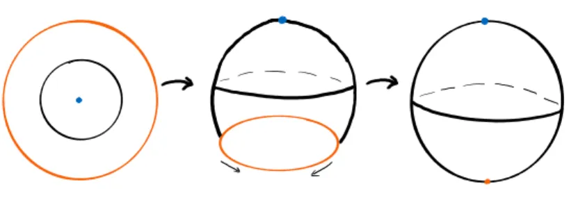
To give a specific example which also plays an important role in the remainder, we consider the homeomorphism between the sphere and the quotient of the disc(square) and its boundary. The explicit map will not be given here, we instead give a sketch of the intuitive idea behind the homeomorphism (see fig.2.1). In the remainder we use all three representations of thed-dimensional sphere

S^d'D^d/∂D^d'I^d/∂I^d.

The definition of homotopy groups in the following section requires to extend the definition of a homotopy to pairs (X, A) of a topological space and a subspace. Consider pairs (X, A) and (Y, B) withA⊆XandB⊆Y, a mapf: (X, A)→(Y, b) is a map f:X→Y with the property thatf(A)⊆B. In the definition of homotopy groups the subspace will be just a distinguished point, calledbase point,x0∈X.

A mapf: (X, x0)→(Y, y0) is mapf:X→Y, such thatf(x0) =y0and a homotopyF between two such maps is calledbase point preservingifF(x0, t) =y0 for allt∈[0,1].

More generally, a homotopy between two mapsf0, f1 : (X, A)→(Y, B) respects the subset structure andF(A, t)⊆B∀t∈I.

We denote the set of equivalence classes of mapsf: (X, x0)→(Y, y0) with the equivalence relation given by base point preserving homotopies by [(X, x0),(Y, y0)].

(11)

2.1 Homotopy theory

Figure 2.1: Sketch of the idea behind the homeomorphism betweenS^dandD^d/∂D^d. The blue point and the orange circle are mapped to the north and south pole of the sphere, respectively.

Homotopy groups. With the definitions of equivalence classes from the previous section we now want to distinguish a special set of equivalence classes, the so calledhomotopy group. As the name suggests, a well-defined group structure can be given to this set. The homotopy group will be associated to a space with base point (X, x0) and it turns out to be very useful tool in topology. Some applications will be discussed here as examples.

Throughout this work, more applications will become apparent.

Definition 3. Let (X, x0) be a topological space with base pointx0. Thehomotopy groupπd(X, x0) is defined as

πd(X, x0) := [(S^d, s0),(X, x0)].

This defines the homotopy group as a set. Furthermore, we can define a group structure forπd(X, x0). This will be done in the following in detail.

Remark 1. The base pointx0 will often be dropped from the notation since it can easily be shown that the homotopy group does not depend on either base points0or x0. However, it is important to choose one and use the base point preserving property of homotopies. Which specific base point is chosen does not matter.

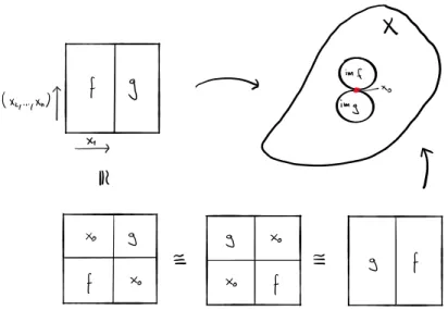
The group structure ofπd(X) can probably best be understood in the representation ofS^d'I^d/∂I^d. SetI= [0,1] and consider two mapsf, g: (I^d/∂I^d,o)→(X, x0). Their product is then defined by the concatenation along any one of the coordinates:

(f∗g)(x1, . . . , xd) :=

f(2x1, . . . , xn) for 0≤x1≤1/2

g(2x1−1, . . . , xn) for 1/2≤x1≤1 . (2.1)

(12)

This definition descends to the level of homotopy classes and defines a group multiplication onπd(X). For a formal proof of this statement see for example [14].

This multiplication turns out to be abelian for higher homotopy groupsd≥2, ford= 1, however, this is not the case. The first homotopy groupπ1(X), also known as thefun- damental group, is the space of based loops inX and the multiplication is given by concatenation of loops, which is not abelian in general.

Figure 2.2 should give an idea of how the group structure looks in dimensionsd≤2 and why it is abelian.

Figure 2.2: Series of homotopies betweenf∗gandg∗fwhich suggests that the group multiplication really is abelian for dimensiond≥2.

Homotopy groups of spheres. Homotopy groups are a great tool to understand the topology of a spaceXand one of the central tasks in homotopy theory is to compute the homotopy groups of spheresπd(Sⁿ). While this question is not very rich ford≤n it becomes more interesting ford > n. The more important case for this work, however, isd≤n, or more preciselyd=nsinceπd(Sⁿ) = 0 for 0< d < nandπn(Sⁿ)'Z.

The simplest casen= 1 is very intuitive and serves as a good example. So forπ1(S¹) we are looking for the homotopy classes of maps fromS¹→S¹. These can be under-

(13)

2.2 Homology theory stood quite intuitively since each one can be characterized by the number of times the circle gets wrapped around another circle. The key observation for this visualization is that the identity map is not homotopic to the constant map to the base point. This shows thatπ1(S¹) is generated by the homotopy class [idS¹] and thusπ1(S¹) =Z.

The argument for the higher dimensional spheres is the same and eachπn(Sⁿ) =Zis generated by the homotopy class of the identity map.

Given a mapf:S^d→S^d, the integer defined by the homotopy class [f]∈πd(S^d) is called themapping degreedeg(f) off. In the cased= 1 this is sometimes calledwinding numberas well.

2.2 Homology theory

The theory introduced in this section, homology theory, and its dual theory are very important tools in topology and have a wide range of applications in theoretical physics.

There are various different versions of homology theory. We will focus on the definition and discussion of singular homology here and roughly follow the introduction of Hatcher in [14] (Sec. 2.1). However, all different versions are based on the general concept of achain complex. We begin with the very basics and general definitions for homology groups, which are the same for all different versions of homology theory. It will also become clear how there can be different versions of homology theories arising from the same basic idea. In the next sections the notions ofcohomology and relative (co)homology are introduced.

Definition 4.Achain complexis a sequence of abelian groupsA0, A1, A2, . . .connected by homomorphisms∂n:An→A_n−1, such that∂_n−1◦∂n= 0 for alln. It may be written in the form

· · · ←A0

∂1

←−A1

∂2

←−A2

∂3

←−A3←. . . . We will also write (Ai, ∂i) in short.

Elements in the kernel of∂are calledcycles(or closed elements) and elements in the image of∂are calledboundaries(or exact elements). By definition every exact element is closed, i.e. im(∂n+1)⊆ker(∂n). And with that the homology groupHn(Ai, ∂i) of a chain complex is defined as

Hn(Ai, ∂i) := ker(∂n)/im(∂n+1). (2.2) Note that Hn is always a well defined group since we started by considering abelian groupsAi.

As stated above, the notion of a chain complex can be defined for different objectsAi

and this gives rise to different notions of homology.

We take this opportunity to mention the somewhat related notion of anexact sequence, which is frequently used in algebraic topology. Consider a sequence of groupsAi(not

(14)

necessarily abelian) and group homomorphismfi:Ai→Ai+1. Such a sequence is called exact if for alli

im(fi) = ker(fi+1). (2.3)

Note that this definition can be made for other algebraic structures as long as kernel and cokernel make sense.

Exact sequences have a wide range of application in algebraic topology and they . More details will be discussed when needed and we leave it with the general introduction at this point.

Now, to introduce the notion of singular homology, we start with the basic building blocks:

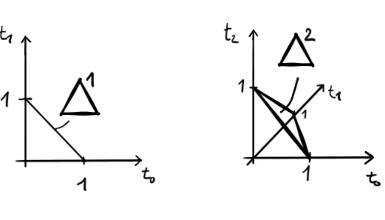
Definition 5. The standardn-simplex is defined as the set

∆ⁿ:={(t0, . . . , tn)∈Rⁿ⁺¹|X

i

ti=i andti>0∀i}. (2.4) Note that the ordering of indices determines an orientation on the edges according to increasing indices.

The (n−1)-simplex ∆ⁿ_i⁻¹obtained by omitting thei-th vertex of ∆ⁿis a face of ∆ⁿ and is (canonically) isomorphic to ∆ⁿ⁻¹. The boundary∂∆ⁿof ∆ⁿis given by the union of alln−1 faces and the openn-simplex ˚∆ⁿis ∆ⁿ−∂∆ⁿ.

Asingular n-simplex in a topological spaceX is a continuous mapσ : ∆ⁿ →X.

LetCn(X) be the free abelian group with the singularn-simplices inXas a basis. An element ofCn(X) is called(singular)n-chainand is a finite formal sumP

iniσiwith ni∈Zandσi: ∆ⁿ→X. The boundary map∂n:Cn(X)→Cn−1(X) is defined in the following way:

∂n:Cn(X)→Cn−1(X) σ7→∂n(σ) =

Xn i=0

(−1)ⁱσ|∆ⁿ⁻¹_i .

This definition implies the canonical isomorphism ∆ⁿ_i⁻¹'∆ⁿ⁻¹ mentioned before, so thatσ|∆ⁿ⁻¹_i is indeed a singular (n−1) simplex.

Lemma 1. The composition of two boundary maps∂n−1◦∂n:Cn(X)→Cn−2(X)is zero.

Proof.Considerσ∈Cn(X). Then

∂n(σ) = Xn i=0

(−1)ⁱσ|∆ⁿ⁻¹_i

(15)

2.2 Homology theory

Figure 2.3: Sketch of the standard 1-simplex and the standard 2-simplex.

and

(∂n−1◦∂n)(σ) = Xn j<i

(−1)ⁱ(−1)^jσ|∆ⁿ⁻¹_ji + Xn j>i

(−1)ⁱ(−1)^j⁻¹σ|∆ⁿ⁻¹_ij = 0. These two sums cancel since exchangingiandjin the second sum gives the negative of the first sum.

This Lemma tells us that the singular chainsCn(X) with the boundary map∂define a chain complex and we can define the homology groupHn^sing(X) of that chain complex.

Remark 2.The standardn-simplex ∆ⁿis homeomorph to then-diskDⁿand its boundary toSⁿ⁻¹. We mention this here, as it might be sometimes more intuitive to consider mapsDⁿ→X, and furthermore a (singular)n-chain is often written as a linear combi- nation of mapsci:Dⁿ→Xin the following sections.

Example. Let us discuss a simple example at this point. Consider the three dimensional spaceX=R³\ {0}with the origin removed. Now, in order to compute the homology groupHn^sing(X), we need to find a closed (singular)n-chain, which is not the boundary of a singular (n+ 1)-chain inX.

Forn= 1 this is not possible, given any closed 1-chain we find a 2-chain, such that its boundary is the considered 1-chain. Forn= 3 this is trivial as well, since there are no 4-chains inR³\ {0}, but there also is no closed 3-chain and thereforeH^sing3 (X) = 0 =

(16)

2 Mathematical preliminaries H1^sing(X).

But forn= 2 things are a little more interesting. There exists a closed 2-chain, which is not the boundary of a 3-chain, namely the 2-chain, which contains the origin on the inside. To be more precise, consider the boundary of the 3-simplex that is located in R³\ {0}such that the origin is on the inside of the tetrahedron. Now, even though you can think of this 2-chain as the boundary of a 3-chain, this 3-chain is not a valid 3-chain in X and this 2-chain generates the homology groupH2^sing(X) =Z.

One might even go further and show thatX'S²and see that we have just computed the homology groups of the 2-sphere – even though we did not worry to much about the details here and a proof of this fact would need a more careful discussion.

An example of a topological invariant based on homology that will be important later on, is the so calledEuler characteristicof a topological SpaceX.

Definition 6. Let X be ad-dimensional topological space and bn := rank(Hn(X)) the so calledn-th Betti number. Then is the Euler characteristicχ(X) defined as the alternating sum

χ(X) :=

Xd i=0

(−1)ⁱbi.

The homology group of a topological space measures topological information in a similar way as the homotopy group, but it is often much easier to compute. This comes with a price, as the homotopy group is the finer tool and can detect information, that the homology group can not detect. The most famous example for this would be the Hopf mapS³→S². But we will not go into more detail here. Nonetheless, the next theorem states a connection between homology and homotopy groups of a spaceX.

2.2.1 The Hurewicz theorem

TheHurewicz theorem is one of the central results in algebraic topology and builds a connection between homotopy theory and homology theory. We will only state the theorem and refer for example to Hatcher [14] for a proof of the statement.

Theorem 2.LetXbe a topological space. Then there exists a group homomorphism for everyk∈N

h∗:πk(X)→Hk(X).

Now, letnbe another positive integer and ifXis path connected andπk(X) = 0for all k < nthenh_∗ is an isomorphism for allk≤n(forn≥2and the abelianization for n= 1.

We do not go into more detail on this topic as it is not of importance for this work, but it still worth to mention the established connection between the two topics introduced before.

(17)

2.2 Homology theory

2.2.2 Cohomology groups

Cohomology groupsare another different invariant that can be assigned to a topological space and are closely related to homology groups. As it was the case for homology there exist various different versions of cohomology. Even more as for homology. As the name suggests, some of them can be obtained from a homology theory by dualizing. We will start with the basic idea and the general definition ofcochain complex(very similar to chain complexes).

Definition 7. Acochain complex is a sequence of abelian groupsA0, A1, A2, . . . connected by homomorphismsdn:An→An−1, such thatdn+1◦dn= 0 for alln. It may be written in the form

· · · →A0 d0

−→A1 d1

−→A2 d2

−→A3→. . . .

Elements in the kernel ofdare calledcocycles (or closed elements) and elements in the image ofdare calledcoboundaries (or exact elements). By definition every exact element is closed, i.e. im(dn)⊆ker(dn+1). And with that the cohomology groupHⁿof a cochain complex is defined as

Hⁿ:= ker(dn)/im(dn−1). (2.5) As it was the case for a chain complex, the notion of a cochain complex can be defined for different objects and gives rise to the different notions of cohomology.

Example. A first example of this is the cochain complex of differential forms on a man- ifoldMwith the exterior derivatived: Ωⁿ(M)→Ωⁿ⁺¹(M). The cohomology associated to this cochain complex is usually calleddeRham cohomologyHdRⁿ (M).

For any chain complex there exists a cochain complex, obtained by dualizing. That means replacing every groupAiby its dual groupA^∗_i:= Hom(Ai, R), for a fixed abelian groupR, and every homomorphism∂iby the dual homomorphism

di−1:A^∗i−1→A^∗i, f7→f◦∂ .

Singular cohomology. Starting from n-chains (Cn(X), ∂), a singular cochain can be defined asCⁿ(X;R) := Hom(Cn(X), R). The coboundary operatordis then defined as the dual of the boundary operator∂and the cohomology group as

H_singⁿ (X;R) := ker(dn)/im(dn−1). (2.6) We usually work with the coefficients beingR=Z. However, in the section on obstruc- tion theory, the obstruction cochain will be constructed as a cochain with coefficients in some homotopy groupπk(Y). In that case one needs to have the restrictionk≥2 for the homotopy group to be abelian.

(18)

2.2.3 Relative (co-)homology

There also is a relative version of homology. Consider a pair (X, A) withA⊆X. Since chains inAare obviously also chains inX, we have thatCn(A) is a subgroup ofCn(X) and therefore define

Cn(X, A) :=Cn(X)/Cn(A). (2.7) The boundary operator∂descends to a map∂:Cn(X, A)→Cn−1(X, A) and is still a well defined boundary map. The homology group of this chain complex is then defined as

Hn^sing(X, A) := ker(∂|Cn(X,A))/im(∂|Cn+1(X,A)). (2.8) With the definition ofCn(X, A) (2.7) there is an intuitive way to picture representatives of elements inHn^sing(X, A) as chainscinXwhose boundary∂clies inA. This means elements inCn(X, A) do not need to be closed, but their boundary needs to be inCn−1(A).

The relative version of cohomology can be introduced in a similar way as before by dualizing the relative homology. And even for cohomologies, such as deRham cohomology, which are not obtained by dualizing, a relative version can usually be defined. For more details on the relative version of deRham cohomology consider for example Bott and Tu [4], chapter 1.6.

With the definition of relativen-chainsCn(X, A) (2.7) comes a (short) exact sequence 0→Cn(A)−→ⁱ Cn(X)−→^p Cn(X, A)→0, (2.9) with the inclusion i : Cn(A) ,→ Cn(X) and the projection on equivalence classes p:Cn(X)→Cn(X)/Cn(A).

This is indeed an exact sequence. To see this, note that the inclusion is injective and therefore ker(i) = 0. The projection pis surjective which proves the exactness at Cn(X, A). The missing part is to show that ker(p) = im(i) which is clear from the definition ofCn(X, A) =Cn(X)/Cn(A).

2.3 Obstruction theory

Obstruction theory does not play a major role in the remainder of this work, but it is, however, quite a useful tool to prove, for example, the existence of a homotopy. It is necessary to give a brief introduction to CW complexes for the definition of obstruction theory due to Eilenberg [12]. Nonetheless, CW complexes are an interesting topic on their own and they have many applications in algebraic topology. After the definition of CW complexes and an example of the torus as CW complex, the notion of cellular homology is introduced and followed by the basic idea of obstruction theory in terms of an extension problem.

(19)

2.3 Obstruction theory CW complexes. A CW complexXis often defined by an inductive construction process. This is quite instructive and gives a good intuitive understanding of CW complexes and therefore it is presented here. The idea is to build up a spaceXwith cells of increasing dimension. Vice versa, one could think of this as the decomposition of a space Xinto cells.

Let us begin with a set of 0-cellsX0. We call it the0-skeletonof a spaceX.

Now, we continue with one dimensional cells and attach any number of 1-cells via continuous mapsfi:∂D¹→X0to obtain the 1-skeletonX1. In other words, we can think of this as the process of

”gluing“ 1-cellsc'D¹= [0,1] into the 0-skeleton by assigning to each endpoint of the 1-cell one point inX0via the mapsfi. If both endpoints are mapped to the same pointx∈X0the result is homeomorphic to the circleS¹based at the pointx. In general on could say that the 1-skeleton is agraph.

Next, we obtain the 2-skeleton by attaching 2-cells to the 1-skeleton, again via continuous mapsfi:∂D²→X1.

By continuing in this way, we obtain ann-dimensional spaceX0⊂X1⊂ · · · ⊂Xn, which we call a (finite dimensional)CW complex. This process can even continue infinitely to define an infinite-dimensional CW complex as the direct limit of then-skeleta.

The name CW complex refers to the topology defined for such a space, where C stands forclosure finiteand W for weak topology. The technical details are not of importance here and can, alongside an introduction and further examples, be found for example in [14].

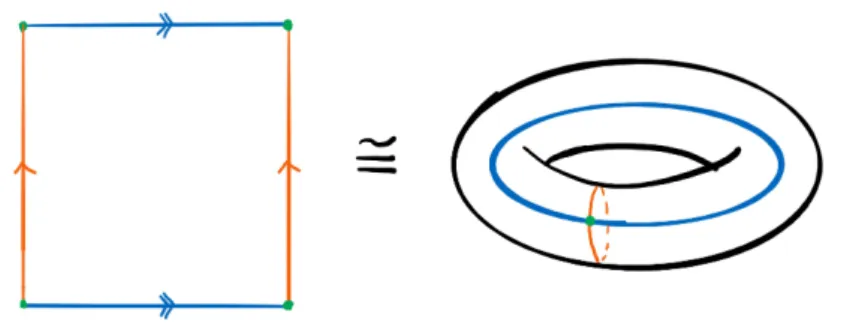
Example. One example of a CW complex that plays a central role in this work is the torusT^d. To consider a tangible example let us setd= 2. The construction works similarly for all dimensionsd.

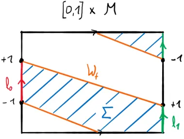
The 0-skeleton of the 2-torus is just a single point{x0}=X0. The 1-skeleton consists of two 1-cells attached toX0by the continuous mapf:S⁰→X0which maps both points ofS⁰tox0∈X0. Finally, one 2-cell is attached via a continuous mapf:S¹→X1. The attaching mapfcan best be understood visually in figure 2.4. The gluing mapfmaps the boundary of the discD²to the boundary of the square in the left figure of fig. 2.4.

And since the boundary is build out of two 1-cells, it would first follow the blue 1-cell, then the orange 1-cell, then the blue 1-cell, but in reverse direction and finally the orange 1-cell also in reverse direction. In this fashion the interior of the square represents the two cell of the CW structure of the torus. In the right figure of fig.2.4 the torus is shown in its usual representation (embedded inR³).

Cellular homology. Given a CW complex we can define a chain complex associated to it. To this chain complex we can define the homology in the usual way and this is called cellular homology. The definition of this chain complex makes use of the construction of then-skeleton from the (n−1)-skeleton and it turns out that cellular homology groups

(20)

Figure 2.4: CW structure of the torus. The green dot represents the 0-skeleton, the two 1-cells are shown in orange and blue (in the left figure two opposite edges are identified) and the 2-cell is given by the interior of the square.

are quite easy to compute. To demonstrate this, the example of the torus comes up again and its homology groups are computed in this context. For a somewhat more detailed discussion of this topic consider again for example the book of Hatcher [14]

LetX be a CW-complex and consider the short exact sequence associated to the relative chain groupCn(Xn, Xn−1):

0→Cn(Xn−1)−→ⁱ Cn(Xn)−→^p Cn(Xn, Xn−1)→0. (2.10) To any short exact sequence of chain complexesC_∗(Xn) there exists a long exact sequence in homology, ifiandpare chain maps, i.e. commute with with the boundary operator:

· · · →Hk(Xn−1)→Hk(Xn)→Hk(Xn, Xn−1)→Hk−1(Xn−1)→Hk−1(Xn)→. . . . (2.11) Arranging parts of the long exact sequences for the pairs (Xn+1, Xn), (Xn, Xn−1) and (Xn−1, Xn−2) in the correct way lets us define thecellular chain complex

· · · →Hn+1(Xn+1, Xn)→Hn(Xn, Xn−1)→Hn−1(Xn−1, Xn−2)→. . . . (2.12) The concatenation of two maps is zero, because it contains two successive maps in one of the long exact sequences. Therefore, it is indeed a chain complex and the homology groups of this chain complex are calledcellular homology groupsHn^CW(X). In fact the following theorem holds.

(21)

2.3 Obstruction theory Theorem 3. LetXbe a CW-complex. Then the homology groupsHn(X) =Hn^CW(X) for alln.

Note, that ifXhask n-cells, thenHn(Xn, Xn−1) is a free abelian group generated bykelements and therefore alsoH^CW(X) is generated by at mostkelements. Also, since elements inHn(Xn, Xn−1) are equivalence classes ofn-cells inXnit often becomes fairly easy to explicitly compute the cellular homology groups as many CW complexes of interest have only finite skeleta. This becomes more clear in the following example.

Before we return to the example of the torus, there is another interesting fact for CW complexes worth mentioning here: The Euler characteristic of a CW-complex can be defined as the alternating sumχ(X) =k0−k1+k2−k3+. . ., whereknis the number ofn-cells in the complex. This is not really a definition, but it can be deduced from the previous definition of the Euler characteristic.

Example. Consider again the example of a torus, but this time the 3-torusT³=S¹× S¹×S¹. Its CW structure is given by one 0-cell, three 1-cells, three 2-cells and one 3-cell. The cellular chain complex is thus of the form

0→Z→Z³→Z³→Z→0.

It turns out that all three maps in this chain complex are the zero map and the homology groups of the torus are therefore given byHi(T³) =Z, fori= 0,3 andHi(T³) =Z³, for i= 1,2.

Recall the definition of the Euler characteristic from the previous section: χ(X) = P

i(−1)ⁱbi. Now, that we have computed the homology groups of the three torus, we can as well compute the Euler characteristic of the three-torus asχ(T³) = 1−3+3−1 = 0.

As it turns out this is true for any dimension andχ(T^d) = 0 for alld.

We want to take the opportunity at this point to introduce a notion which will be important for later. A subtorus of a torusT^dis a (d−1)-dimensional torusT^d⁻¹⊂T^d. In case ofd= 3, consider a parametrization

(0,2π)³→T³=S¹×S¹×S¹ (θ1, θ2, θ3)7→(eîθ¹, eîθ², eîθ³).

Then a subtorus can for example be obtained by fixing one of the angles. For later pur- poses we call a subtorus, whereθ1is fixed, a 23-subtorus (or ayz-torus). Analogously for thezx- andxy-subtori.

Extension problem. The basic question we seek to answer is wether a continuous map f, defined on a subsetA⊂X, can be extended to a continuous map ˜fon all ofXwith f|˜A≡f or not. IfXandAare CW complexes, we can first look at the simpler case,

(22)

wherefis defined on then-skeleton and the question can be if it can be extended over the (n+ 1)-skeleton. In other words, we are looking for an inductive process of extending fover then-skeleta ofX.

Assume thatf:Xn→Y is a continuous map defined on then-skeleton ofX. The (n+ 1)-skeletonXn+1is constructed fromXnby attaching some (n+ 1)-cells to it via continuous mapsϕi: (Dⁿ⁺¹, Sⁿ)→(Xn+1, Xn) (i= 1, . . . , k). Note, thatf◦ϕi:Sⁿ→Y and [f◦ϕi]∈[Sⁿ, Y] =πn(Y) is a collection of elements of then-th homotopy group ofY. Therefore, one can define a (n+ 1)-cochain by assigning to each (n+ 1)-cell the homotopy class of the map defined on its boundary. This defines an (n+ 1)-cochain θⁿ⁺¹(f) with values inπn(Y), soθⁿ⁺¹(f) ∈Cⁿ⁺¹(X;πn(Y)). In fact, ifθⁿ⁺¹(f) is defined this way, the following Lemma holds.

Lemma 4. Letf:Xn→Y be a continuous map defined on then-skeleton ofX. Then the above defined cochainθⁿ⁺¹(f)is a cocyle, i.e.δθⁿ⁺¹(f) = 0.

Returning to the question in the beginning, assume thatf:A→Y is defined on a subsetA⊂X. We can follow the inductive process from above, but in the definition of θⁿ⁺¹(f) we define it to be 0 on (n+ 1)-cells inCn+1(A), sincefis already defined onA.

This wayθⁿ⁺¹(f) defines a cocyle in the relative cohomology groupHⁿ⁺¹(X, A;πn(Y)).

With this the main theorem of obstruction theory can be formulated:

Theorem 5.Let(X, A)be relative CW complex. Letf:Xn→Y be continuous map.

Then the cellular cocycle θ(f) ∈ Cⁿ⁺¹(X, A;πn(Y))which vanishes if and only if f extends to a mapXn+1→Y.

If and only if[θ(f)]∈Hⁿ⁺¹(X, A;πn(Y))vanishes, there exists a mapgwithg|Xn−1= f|^Xn−1and homotopic tofonXnsuch thatgextends overXn+1.

2.4 Vector bundles and vector fields

Vector bundles and vector fields are the key ingredients in the Euler chain representation of a Weyl semimetal. Therefore, we give a brief introduction to the topic and the basic definition for the concepts that will be discussed in the main chapter of this work. Vector bundles in general play a very important role in many areas of theoretical physics and give a good mathematical description of various physical phenomena. The introduction here is for the purpose of this work and is probably not a sufficient basis for all physics literature. There are various mathematical and also physics textbooks on this topic that give a more detailed introduction see for example [4] or [15].

2.4.1 Vector bundles

We start with a slightly more general definition of vector bundles, even though we will only consider vector bundles over manifolds.

(23)

2.4 Vector bundles and vector fields Definition 8.LetMandEbe topological spaces. Avector bundle(E, M, π) is given by a base spaceM, the total spaceEand the continuous surjectionπ:E→M(projection) and the condition that for everyp∈M the fiberπ⁻¹(p) has the structure of a finite dimensional real (or complex) vector space. Furthermore, there exist an open neighbor- hoodUfor everyp, a natural numberkand a homomorphismφ:U×R^k→π⁻¹(U), such that

• π◦φ(p, v) =x ∀v∈R^k

• v7→φ(p, v) is a linear isomorphism for allp∈M .

The open setUand the mapφare called alocal trivialization(U, φ).

Given twocharts(Ui, φi) and (Uj, φj) there is a linear isomorphism for everyp∈Ui∩Uj

gji(p) :=φj◦φ⁻_i¹|^p:R^k→R^k,

Which is calledtransition function. Note, that these transition functions have the property

gii≡1, gij◦gjk=gik. (2.13) Given two vector bundles (E1, M1, π1) and (E2, M2, π2) a morphism between two vector bundles is a pair of mapsf:E1→E2andg:M1→M2, such thatπ2◦f=g◦π1

and that for everyp∈M1the mapπ⁻₁¹(p)→π₂⁻¹(g(p)) induced byfis a linear map of vector spaces.

E1 E2

M1 M2

f

g

π1 π2

Next, we introduce two operations on vector bundles, theWhitney sum(or direct sum) and thetensor productof two vector bundles. For that let (E1, M, π1) and (E2, M, π2) be two vector bundles overM.

A prominent example of a vector bundle is the tangent bundleT Mof a manifoldM.

This bundle is defined as the collection of all tangent spacesTpMat allp∈Mand it is usually one of the first examples one encounters.

Definition 9.Let (E, M, π) be a vector bundle. A (global) section of a vector bundle is a maps:M→Esuch that (π◦s)(p) =p ,for allp∈M.

The set of all (global) sections of a vector bundle is denoted by Γ(E). This set contains at least one section, the zero section.

Remark 3.In the case of a (more general) fiber bundle there does not need to exist a global section. It makes sense to define the notion of local section in this case.

(24)

2.4.2 Vector fields

Returning to the previous example of the tangent bundle of a manifoldT M, a section v∈Γ(T M) associates a tangent vectorv(p) to every pointp∈M, so sections in Γ(T M) are (tangent) vector fields onM.

There are many results on vector fields on a manifoldM. The most important results for this work will be stated here.

Definition 10. Letv∈Γ(T M) be a vector field with an isolated zero atp∈M. The indexofvatpindexp(v) is defined to be the degree of the map

S^dp⁻¹→S^d⁻¹, x7→ v(x)

|v(x)|,

whereSp^d⁻¹ is the boundary ∂Dpof a small ball centered around p∈M, such that v(x)6= 0∀x∈Dp\p.

There is a famous theorem which relates the index of vector field onMto the Euler characteristic ofM.

Theorem 6. (Poincar´e-Hopf ). Let M be a compact differentiable manifold. Let v∈Γ(T M)be a vector field onM with isolated zeroes. Then

X

i

indexpi(v) =χ(M),

where the sum is over all isolated zeroes andχ(M)is the Euler characteristic ofM.

(25)

3 Weyl semimetals

This chapter gives an introduction to the topic of Weyl semimetals and Weyl superconductors and sets the stage for the main part of this work. We introduce the setting which is used in the classification of disordered fermion systems with a quadratic Hamiltonian.

Even though the framework and classification addresses disordered fermions, disorder is not introduced explicitly in this first part of this work. In the second part, disorder will play a more prominent role and it will be introduced accordingly there. But even if disorder is not explicitly considered in this first part, it is always considered as an important part of physical systems and should be kept in mind.

The introduction to the general setting is split into three parts, first the step from the single-particle Hilbert space to the many body Fock space is done. Next, the notion of symmetry and symmetry groups and their action in the many body framework are introduced. The third part then explicitly introduces the translation group of the lattice and consequences for translationally invariant systems, since we will assume translational invariance throughout this first part.

This chapter then closes with a short overview over so called Dirac materials, which are materials where the low energy excitations are Dirac or Weyl fermions. Furthermore, the notion of Dirac and Weyl points are introduced and a few remarks on their basic properties are made.

3.1 Many-body framework

The systems under consideration are semimetals and superconductors and they consist of a vast number of interacting particles (of the order 10¹⁰−10²⁵). The theory ofmany- body quantum mechanicsintroduces a formalism to treat such systems in a satisfactory way. As was already mentioned we will focus on quadratic Hamiltonians and thus we are only considering interactions described by mean-field theory and neglecting all further contributions. In the Physics literature and more specific in the context of insulators, semimetals and superconductors this is known as the Hartree-Fock-Bogoliubov approximation.

Another central ingredient is the symmetry groupG. Symmetries play a very important role in all areas of physics and they obviously are very important for the idea of a symmetry classification. Dyson’s threefold way [10] is a very famous result of a symmetry classification for free fermions and the extension done by Heinzner, Huckleberry and Zirnbauer [16] is inspired by Dyson’s original approach. Besides the general frameork, the symmetry groupGand its action will be part of this introduction and the overall framework. The introduction given here is somewhat based on [16] since the framework is similar, it is however still very useful to give a detailed overview of the basic definitions

(26)

3 Weyl semimetals

here, as some specifics and details of the framework are different.

The first important step to extend the setting introduced in Dyson’s threefold way [10] is the passing from single-particle quantum mechanics to the framework of many- body quantum mechanics. This usually goes under the name of second quantization.

Here, we want to lay out the mathematical foundation of this procedure in a concise way.

Our starting point is the single-particle Hilbert spaceVwith Hermitian scalar product h·,·iV. For simplicity only finite-dimensional vector spacesV =C^N will be considered here. The Hermitian structure defines an isomorphism betweenV and its dual space V^∗, which is given byφ:V →V^∗, v7→ hv,·i^V (also known as Frechet-Riesz isomorphism). Furthermore, it determines a unitary groupU(V), which is the group ofC-linear operatorsgsatisfyinghv, wi=hg(v), g(w)ifor allv, w∈V.

Remark 4. The finite-dimensional Hermitian vector space and its unitary group are two ingredients for Dyson’s threefold way [10] – the missing ingredient is an anti-unitary transformation such as time-reversal. There are more details on that in the section on symmetry classification later on.

Now, let us pass from the single-particle settingV to the fermionic Fock spaceV (V) of many-body quantum mechanics. The Fock space is graded by the particle number V(V) =L

nVn

(V) and then-particle subspaceVn

(V) carries an induced Hermitian structure, given by

hv1∧ · · · ∧vn, w1∧ · · · ∧wni:= Det





hv1, w1i · · · hv1, wni ... . .. ... hvn, w1i · · · hvn, wni



.

With this, the fermionic Fock space itself has the structure of a Hilbert space.

There are two important operations on the Fock space: exterior multiplication by v∈V

ε(v) :^n

(V)→^n+1

(V) andcontractionbyϕ∈V^∗

ι(ϕ) :^n

(V)→^n−1

(V)

with the physical interpretation of creating and annihilating a particle.

Let{ei}i=1,...,Nbe a basis ofV and{fi}i=1,...,Nbe the dual basis ofV^∗withfi(ej) =δij

then the standard physics notation is to writec^†i :=ε(ei) for creation operators and ci:=ι(fi) for annihilation operators. Some algebra reveals that these operators satisfy the so calledCanonical Anti-commutation Relations(or CAR for short)

c^†ic^†j+c^†jc^†i= 0 =cicj+cjci, c^†icj+cjc^†i=δij. (3.1)

(27)

3.1 Many-body framework These relations are in fact the representation of the underlying Clifford algebra relations of the Clifford algebra Cl(W, B) of the vector spaceW:=V⊕V^∗with the symmetric bilinear form

{v+ϕ, v⁰+ϕ⁰}=ϕ⁰(v) +ϕ(v⁰). (3.2) This representation of the Clifford algebra Cl(W,{,}) on the Fock spaceV(V) defined above is calledSpinor representation. The vector spaceW=V⊕V^∗in this context is often known as theNambu space, or the space offield operatorsψ.

Besides the symmetric bilinear form{·,·} there is another important structure on W, which is the real structureγ. A real structure (C-antilinear involution) onW is determined by the Hermitian scalar producth ·,·i^V onV

γ:W→W, v+ϕ7→φ⁻¹ϕ+φv . (3.3) In physics language the spaceWR:= fixW(γ) is usually called the space ofMajorana fields. It is the real vector space spanned by the Majorana operatorsek+fkand iek−ifk. Each of these to structures induces an action on the linear transformations L ∈ End(W). Forγthis is given by

L7→γ◦L◦γ ,

which defines an anti-linear involution on End(W). And we can define a linear anti- involutionL7→L^T calledtransposition and defined through the relation

{ψ, L^Tψ⁰}={Lψ, ψ⁰},∀ψ, ψ⁰∈W .

Using these two structures, we can define a Hermitian structure on the the Nambu space h·,·i^W. Letw, w⁰∈W, then

hw, w⁰i:={γw, w⁰} defines a natural Hermitian scalar product onW.

The reason to introduce the Nambu space is to simplify the process of classification.

The classification according to the tenfold way is guided by the question

”what is the structure of the set ofone-body time evolutions ofV

(V) which commute with a given G-action?“[33]. Therefore, we are interested in one-body, or quadratic (in the creation and annihilation operators), self-adjoint HamiltoniansH:

H=1 2

X

lm

Ylm(c^†_lcm−cmc^†_l) +1 2

X

lm

Zlmc^†_lc^†m+ ¯Zlmcmcl. (3.4) It makes much more sense to consider the anti-hermitian operators iHinstead ofH. This might seem like a trivial modification, but unlike hermitian operators the anti-hermitian operators are closed under the commutator and Hamiltonians iHof the form (3.4) form the Lie algebra Cl2(WR) of skew-symmetrized elements of degree 2. This can easily be verified asWR is spanned by Majorana operatorsck+c^†_kand ick−ic^†_kand a general

(28)

3 Weyl semimetals

skew-symmetrized product of two elementsX, Y ∈WR⊂Cl(WR) can be written in the formiHwith Has in eq.(3.4). Exponentiating this Lie algebra gives the Spin group Spin(WR) and therefore time evolutionsU=e⁻^iHt/^~are elements in Spin(WR).

The isomorphism of the Lie algebras Cl2(WR)'so(WR) exponentiates to a mapping on the level of Lie groupsρ: Spin(WR)→SO(WR), given byρ(g)v=gvg⁻¹forv∈WR. This mapping, however, is not an isomorphism, but is a 2:1 cover, i.e. ρ(−g) =ρ(g).

Nonetheless it is a representation of Spin(WR) on the real vector spaceWR, which can be extended to a representation onW byC-linearity. This fact allows us to study representations of Spin(WR) on the Nambu spaceWinstead of the full Fock spaceV

(V).

3.2 Symmetries

Symmetries play an important role in the understanding of physical systems and they are the fundamental building blocks of the classification of disordered fermions in the so called tenfold way. This approach as well as the name are based on Dyson’s original threefold way. Now, we want to understand how the symmetries are introduced into the many-particle framework established in the previous section and thus build the setting for the tenfold classification.

We already mentioned the unitary groupU(V) determined by the Hermitian structure of our Hilbert spaceV. Now, letG0be the group of unitary symmetries. That means there is some groupG0which acts onV by unitary operatorsρV(g)∈U(V) (we will simply writeρV(g)∼=g). Since the group action is defined onV we equip the Nambu spaceWwith the inducedG0-representation. That means thatV is equipped with the given representation and forf∈V^∗andg∈G0

(g⁻¹)^tϕ=ϕ◦g⁻¹. (3.5)

The groupG0is a normal subgroup of a larger group, the full symmetry groupG. The groupGcontainsG0as a subgroup and, furthermore, elementsgT which act as anti- unitary operatorsT :W →W. These are referred to as distinguished”time-reversal“

symmetries. In fact, moduloG0 there exist at most two such distinguished operators and they satisfyT²=±1.

Every element in the set of anti-unitary elements in the full symmetry group can be written as the right multiplication of a distinguished element, here one of the time reversal operatorsT, with an element ofG0and we can write the enlarged symmetry group asG0∪T G0.

Thus far we introduced the setting of Dyson’s threefold way. However, the Fock space structure allows us to define another anti-unitary operator, that of particle-hole conjugationC, and extend the setting of Dyson

Let Ω be a generator ofVN

(V) withN= dim(V) and normalizationhΩ,Ωi= 1. Then theparticle-hole conjugationis the anti-unitary operatorC:Vn

(V)→VN−n(V) defined

(29)

3.3 Lattice model and translational invariance by the relation

(Cψ)∧ψ⁰=hψ, ψ⁰iΩ.

A simple calculation shows that for aT-invariant choice of Ω, which we can always do, the two operatorsCandTcommute,CT=T C, and also thatCg=gCfor allg∈G0

under the assumption that the vacuum and the fully occupied state are invariant under G0.

Now, we can enlarge the symmetry group even further by allowing a twisted version of particle hole conjugation. This twist can be achieved by an unitary operatorS∈U(V), such thatS²= Id,SΩ = Ω andSG0S⁻¹=G0. Atwistedparticle-hole conjugation then refers to the operator ˜C:=SC=CS. Note, that with the conditions onSwe also have CG˜ oC˜⁻¹=G0and ˜CT=TC.˜

This lets us now write the full symmetry groupGasG=G0∪T G0∪CG˜ 0∪TCG˜ 0, withTC˜= ˜CT, and we call it a minimal extension of Dyson’s setting.

Now, since we want to work on the space of field operatorsW, we need to understand how ˜Cacts onW. ForG0andT this is clear from eq.(3.5), but for ˜Cit takes a little bit more effort. Letψ∈Vn

(V) andψ⁰∈Vn+1

(V) andck, c^†_kannihilation and creation operators for some statek. We want to know what the particle-hole conjugate ˜Cc^†_kC˜⁻¹ ofc^†_kis. Therefore, we do the following calculation

( ˜Cc^†_kψ)∧ψ⁰=hSc^†_kψ, ψ⁰iΩ =hSψ, SckS⁻¹ψ⁰iΩ

= ( ˜Cψ)∧(SckS⁻¹)ψ⁰= (−1)^N−n+1(SckS⁻¹Cψ)˜ ∧ψ⁰.

Thus we see that ˜Cc^†_kC˜⁻¹=±SckS⁻¹∈V^∗, where the sign alternates with the particle number.

Remark 5.Note that for the untwisted particle-hole conjugation this is nothing else than the Frechet-Riesz isomorphismφ:V →V^∗and the full particle-hole symmetry ˜C is equivalent toγ.

3.3 Lattice model and translational invariance

In this section the model used to describe the physical systems under consideration is presented. The more general setting that was laid out in the previous sections will become more specific.

We assume there is periodic lattice indspatial dimensions, which describes the real systems, for example the position of atoms in a crystal, in some approximation. The lattice spacing is assumed to be uniform and, unless explicitly stated otherwise, we assume it to be normalized to 1. Mathematically this lattice can be described byZ^d. To begin again with the single particle-picture, we associate a Hilbert spaceCⁿ, which describes a numbernof complex degrees of freedom, to every point in the lattice. In the tight binding model this leads to the single-particle Hilbert spaceV =`²(Z^d)⊗Cⁿ. For

(30)

3 Weyl semimetals

the following considerations it might be useful to fix a basis forV. We write|x, li ∈Vas the basis elements, wherellabels some orthonormal basis ofCⁿandxlabels the series with a 1 at the positionx∈Z^dand 0 anywhere else.

First, we want to introduce the translation operatorty, which is a unitary operator defined as

ty|x, li:=|x+y, li.

For the majority of the remainder we will assume that translations byZ^dare a symmetry, i.e. that the Hamiltonian commutes withtyfor ally∈Z^d. In the setting of the tenfold way, that means thatZ^d⊂G0is a subgroup of the unitary symmetries.

A translation invariant Hamiltonian will be of the general form H|x, li=X

y,m

hml(y)|x+y, mi, with a matrixh(y) :Cⁿ→Cⁿ.

From quantum mechanics we know, that we can find a simultaneous eigenbasis of allty

and the Hamiltonian defined in terms of the Fourier transform

|k, li:= 1

√2πV X

x

e^ik^·^x|x, li.

Herekis an element of thed-dimensional torusT^dand we introduced a volumeV in order to make{|k, li}into an orthonormal basis.

As a quick check, we can compute ty|k, li= 1

√2πV X

x

e^ik^·^x|x+y, li=e⁻^ik^·^y|k, li. (3.6)

And furthermore,Hhas to leave the eigenspaces oftyinvariant H|k, li= 1

√2πV X

x,y,m

e^ik·xhml(y)|x+y, mi

= 1

√2πV X

x,y,m

e^ik^·^(x⁻^y)hml(y)|x, mi

=X

m

˜hml(k)|k, mi,

with ˜hml(k) :=√¹ 2π

P

ye⁻^ik^·^yhml(y). This form of the Hamiltonian is often known as theBloch Hamiltonianand we will write ˜h(k) simply ash(k), as it should be clear from the context. This also means that the Hilbert spaceV decomposes into the eigenspaces Vkcorresponding to the eigenvaluee^−ik·yof the translation operatorty

V =M

k

Vk.