tscount: An R package for analysis of count time series following generalized linear models

SFB 823

analysis of count time series following generalized linear models

Discussion Paper Tobias Liboschik, Konstantinos Fokianos,

Roland Fried

Nr. 6/2015

Series Following Generalized Linear Models

Tobias Liboschik TU Dortmund University

Konstantinos Fokianos University of Cyprus

Roland Fried TU Dortmund University

Abstract

TheRpackagetscountprovides likelihood-based estimation methods for analysis and modelling of count time series following generalized linear models. This is a flexible class of models which can describe serial correlation in a parsimonious way. The conditional mean of the process is linked to its past values, to past observations and to potential covariate effects. The package allows for models with the identity and with the logarithmic link function. The conditional distribution can be Poisson or Negative Binomial. An important special case of this class is the so-called INGARCH model and its log-linear extension. The package includes methods for model fitting and assessment, prediction and intervention analysis. This paper summarizes the theoretical background of these methods with references to the literature for further details. It gives details on the implementation of the package and provides simulation results for models which have not been studied theoretically before. The usage of the package is demonstrated by two data examples.

Keywords: intervention analysis, mixed Poisson, model selection, prediction, R, regression model, serial correlation.

1. Introduction

Recently, there has been an increasing interest in regression models for time series of counts and a quite considerable number of publications on this subject has appeared in the literature.

However, most of the proposed methods are not yet available in statistical software packages and hence they cannot be applied easily. We aim at filling this gap and publish a package named tscount for the popular free and open source software environment R(RCore Team 2014).

In fact, our main goal is to develop software for models that include a latent process similar to the case of ordinary generalized autoregressive conditional heteroscedasticity (GARCH) models (Bollerslev 1986).

Count time series appear naturally in various areas whenever a number of events per time period is observed over time. Examples showing the wide range of applications are the daily number of hospital admissions from public health, the number of stock market transactions per minute from finance or the hourly number of defect items from industrial quality control.

Models for count time series should take into account that the observations are nonnegative integers and they should capture suitably the dependence among observations. A convenient and flexible approach is to employ the generalized linear model (GLM) methodology (Nelder and Wedderburn 1972) for modeling the observations conditionally on the past information,

choosing a distribution suitable for count data and an appropriate link function. This approach is pursued in detail byFahrmeir and Tutz(2001, Chapter 6) andKedem and Fokianos (2002, Chapters 1–4), among others.

Another important class of models for time series of counts is based on the thinning operator, like the integer autoregressive moving average (INARMA) models, which, in a way, imitate the structure of the common autoregressive moving average (ARMA) models (for a recent review seeWeiß 2008). Another type of count time series models are the so-called state space models. We refer to the reviews of Fokianos (2011), Jung and Tremayne (2011), Fokianos (2012), Tjøstheim(2012) andFokianos(2015) for an in-depth overview of models for count

time series.

In the first version of the tscount package we provide likelihood-based methods for the framework of count time series following GLMs. For independent data or some simple dependence structures of low order these models can be fitted with standard software for GLMs (see Section A.2); for example the R function glm produces accurate results. The implementations in our packagetscount allows for a more general dependence structure which can be specified conveniently by the user. Accordingly we fit time series models which include a latent process, similarly to the GARCH class of models. The usage and output of our functions is inspired by theRfunctions glmand arima. We provide many standardS3 methods which are known from other functions. The relatedRpackageacp(Siakoulis 2014) has been published recently and provides maximum likelihood fitting of a simplified first order version of models that we consider. Our packagetscount covers a much wider class of models and includes this model as a special case.

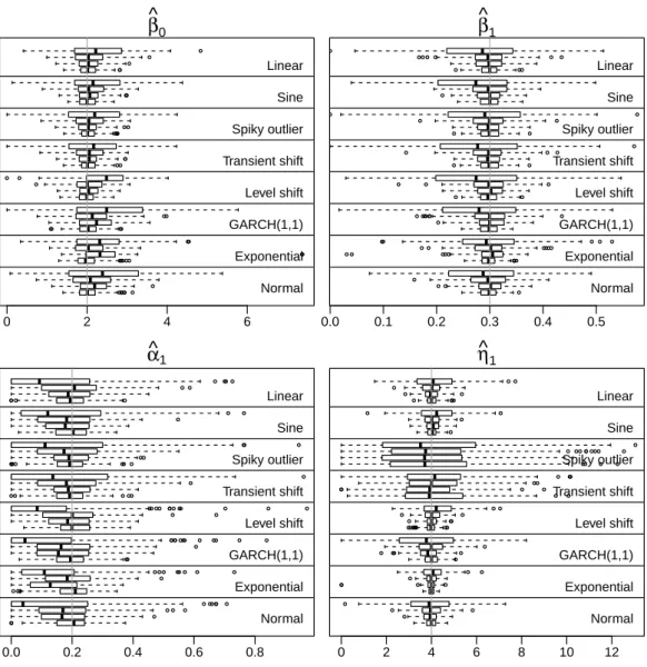
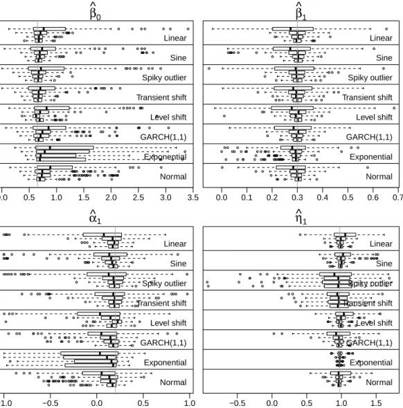
The functionality of our package tscount partly goes beyond the theory available in the literature since theoretical investigation of these models is still an ongoing research theme.

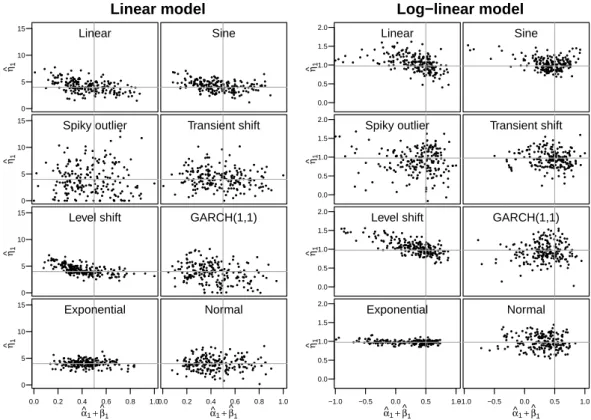
For instance consider the problem of accommodating covariates in such GLM-type count time series models or fitting a mixed Poisson log-linear model. These topics have not been studied theoretically. We have checked their appropriateness by simulations reported in AppendixB.

However, some care should be taken when applying the package’s programs to situations which are not covered by existing theory.

This paper is organized as follows. At first the theoretical background of the methods included in the package is briefly summarized with references to the literature for more details. Section2 introduces the models we consider. Section3describes quasi maximum likelihood estimation of the unknown model parameters and gives some details regarding its implementation. Section4 treats prediction with such models. Section5sums up tools for model assessment. Section 6 discusses procedures for detection of interventions. Section 7 demonstrates the usage of the package with two data examples. Finally, Section8gives an outlook on possible future extensions of the package. In the Appendix we give some additional details and confirm by simulation some of the new methods which have not yet been treated theoretically in the literature.

2. Models

Denote a count time series by tYt :tPNu. We will denote by tXt:t PNu a time-varying r-dimensional covariate vector, sayXt pXt,1, . . . , Xt,rq^J. We model the conditional mean EpY_t|F_t1q of the count time series by a latent mean process, say tλ_t : t P Nu, such that

EpY_t|F_t1q λ_t. Denote byF_t the history of the joint process tY_t, λ_t,X_{t 1} :t PNu up to timet including the covariate information at timet 1. The distributional assumption forYt

given F_t1 is discussed later. We are interested in models of the general form gpλ_tq β₀

¸p k1

β_krgpY_tikq

¸q

`1

α_{`</sub>gpλ<sub>tj`}q η^JX_t, (1) where g : R Ñ R is a link function and rg : R Ñ R is a transformation function. The parameter vectorη pη₁, . . . , η_rq^J corresponds to the effects of covariates. In the terminology of GLMs we call νt gpλtq the linear predictor. To allow for regression on arbitrary past observations of the response, define a setP ti1, i2, . . . , ipu withpPN0 and integers 0 i1  i₂. . . i_p   8. This enables us to regress on the lagged observations Y_ti1, Y_ti2, . . . , Y_tip. Analogously, define a setQ tj1, j2, . . . , jquwithqPN0 and integers 0 j1  j2. . . jq  8 for regression on lagged latent meansλtj1, λtj2, . . . , λtjq. This more general case is covered by the theory for models withP t1, . . . , pu andQ t1, . . . , qu, which are usually treated in the literature, by choosingp andq sufficiently large and setting unnecessary model parameters to zero.

We give several examples of model (1). Consider the situation wheregandrgequal the identity, i.e.,gpxq rgpxq x. Furthermore, let P t1, . . . , pu, Q t1, . . . , qu and η0. Then we obtain from (1) that

λ_tβ₀

¸p k1

β_kY_tk

¸q

`1

α_{`</sub>λ<sub>t`}. (2)

Assuming further thatY_tgiven the past is Poisson distributed, then we obtain aninteger-valued GARCH model of order p andq, in short INGARCH(p,q). These models have been discussed byHeinen(2003),Ferland, Latour, and Oraichi (2006) and Fokianos, Rahbek, and Tjøstheim (2009), among others. Whenη0, then our package fits INGARCH models with nonnegative covariates; this is so because we need to ensure that the resulting mean process is positive.

An example of an INGARCH model with covariates is given in Section6, where we fit a count time series model which includes intervention effects.

Consider again model (1) but now with the logarithmic link function gpxq logpxq,rgpxq logpx 1q and P,Q as before. Then, we obtain alog-linear model of order p and q for the analysis of count time series. Indeed, setν_tlogpλ_tq to obtain from (1) that

νtβ0

¸p k1

βk logpYtk 1q

¸q

`1

α`νt`. (3)

This log-linear model is studied by Fokianos and Tjøstheim (2011), Woodard, Matteson, and Henderson (2011) and Douc, Doukhan, and Moulines (2013). We follow Fokianos and Tjøstheim(2011) in transforming past observations by employing the functionrgpxq logpx 1q, such that they are on the same scale as the linear predictorνt (seeFokianos and Tjøstheim (2011) for a discussion and for showing that the addition of a constant to each observation to avoid zeros does not affect inference). Note that model (3) allows modeling of negative serial correlation, whereas (2) accommodates positive serial correlation only. Additionally, (3) accommodates covariates easier than (2) since the log-linear model implies positivity of the conditional mean processtλ_tu. The effects of covariates on the response is multiplicative for

model (3); it is additive for model (2). For a discussion on the inclusion of time-dependent covariates seeFokianos and Tjøstheim (2011, Section 4.3).

Model (1) together with the Poisson assumption, i.e., Yt|F_t1 Poissonpλtq, implies that PpY_ty|F_t1q λ^y_texppλ_tq

y! , y0,1, . . . . (4)

Obviously, VARpYt|F_t1q EpYt|F_t1q λt. Hence in the case of a conditional Poisson response model the latent mean process is identical to the conditional variance of the observed process.

TheNegative Binomial distribution allows for a conditional variance larger thanλ_t. Following Christou and Fokianos(2014), it is assumed thatYt|F_t1 NegBinpλt, φq, where the Negative Binomial distribution is parametrized in terms of its mean with an additional dispersion parameterφP p0,8q, i.e.,

PpY_ty|F_t1q Γpφ yq Γpy 1qΓpφq

φ φ λ_t

φ λt

φ λ_t y

, y0,1, . . . . (5) In this case,VARpYt|F_t1q λt λ²_t{φ, i.e., the conditional variance increases quadratically withλ_t. The Poisson distribution is a limiting case of the Negative Binomial when φÑ 8. Note that the Negative Binomial distribution belongs to the class of mixed Poisson processes.

A mixed Poisson process is specified by settingY_tN_tp0, Z_tλ_ts, where tN_tu are i.i.d. Poisson processes with unit intensity andtZtu are i.i.d. random variables with mean 1 and variance σ². When tZtuis an i.i.d. process of Gamma random variables, then we obtain the Negative Binomial process withσ²1{φ. We refer to σ² as the overdispersion coefficient because it is proportional to the extent of overdispersion of the conditional distribution. The limiting case ofσ² 0 corresponds to the Poisson distribution, i.e. no overdispersion. The estimation procedure we study is not confined to the Negative Binomial case but to any mixed Poisson distribution. However, the Negative Binomial assumption is required for prediction intervals and model assessment; these topics are discussed in Sections4 and 5.

In model (1) the effect of a covariate fully enters the dynamics of the process and propagates to future observations both by the regression on past observations and by the regression on past latent means. The effect of such covariates can be seen as an internal influence on the data-generating process, which is why we refer to it as an ’internal’ covariate effect. We also allow to include covariates in a way that their effect only propagates to future observations by the regression on past observations but not directly by the regression on past latent means.

FollowingLiboschik, Kerschke, Fokianos, and Fried (2014), who make this distinction for the case of intervention effects described by deterministic covariates, we refer to the effect of such covariates as an ’external’ covariate effect. Lete pe₁, . . . , e_rq^J be a vector specified by the user withei 1 if thei-th component of the covariate vector has an external effect andei0 otherwise,i1, . . . , r. Denote by diagpeq a diagonal matrix with diagonal elements given by e. The generalization of (1) allowing for both internal and external covariate effects then reads

gpλ_tq β₀

¸p k1

β_krgpY_tikq

¸q

`1

α_{`</sub> gpλ<sub>tj`}q η^JdiagpeqX_tj`

η^JX_t. (6) Basically, the effect of all covariates with an external effect is subtracted in the feedback terms such that their effect does enter the dynamics of the process only via the observations. We

refer toLiboschiket al. (2014) for an extensive discussion of internal versus external effects. It is our experience with these models that an empirical discrimination between internal and external covariate effects is difficult and that it is not crucial which type of covariate effect to fit in practical applications.

3. Estimation and inference

Thetscountpackage fits models of the form (1) by quasi conditional maximum likelihood (ML) estimation (functiontsglm). If the Poisson assumption holds true, then we obtain an ordinary ML estimator. However, under the mixed Poisson assumption we obtain a quasi-ML estimator.

Denote by θ pβ₀, β₁, . . . , β_p, α₁, . . . , α_q, η₁, . . . , η_rq^J the vector of regression parameters.

Regardless of the distributional assumption the parameter space for the INGARCH model (2) with covariates is given by

Θ

#

θPR^{p q r 1}: β0 ¡0, β1, . . . , βp, α1, . . . , αq, η1, . . . , ηr ¥0,

¸p i1

βi

¸q j1

αj  1 +

.

The interceptβ0 must be positive and all other parameters must be nonnegative to ensure positivity of the latent mean process. The other condition ensures that the fitted model has a stationary solution (cf.Ferland et al.2006, Proposition 1). For the log-linear model (3) with covariates the parameter space is taken to be

Θ

#

θPR^{p q r 1} : |β1|, . . . ,|βp|,|α1|, . . . ,|αq|  1,

¸p i1

βi

¸q j1

αj

 1

+ .

This is intended to be the generalization (for model order p,q) of the conditions |β1|   1,

|α1|   1 and |β1 α1|   1, which Douc et al. (2013, Lemma 14) derive for the first order model. Christou and Fokianos (2014) point out that with the parametrization (5) of the Negative Binomial distribution the estimation of the regression parametersθ does not depend on the additional dispersion parameterφ. This allows to employ a quasi maximum likelihood approach based on the Poisson likelihood to estimate the regression parametersθ, which is described below. The nuisance parameterφis then estimated separately in a second step.

The log-likelihood, score vector and information matrix are derived conditionally on pre- sample values of the time series and the latent mean processtλtu. An appropriate initialization is needed for their evaluation, which is discussed in the next subsection. For a stretch of observationsy py₁, . . . , y_nq^J, the conditional quasi log-likelihood function, up to a constant, is given by

`pθq

¸n t1

logp_tpy_t;θq9

¸n t1

y_tlnpλ_tpθqq λ_tpθq , (7) where ptpy;θq PpYty|F_t1q is the p.d.f. of a Poisson distribution as defined in (4). The latent mean process is regarded as a functionλ_t: ΘÑR and thus it is denoted by λ_tpθq for allt. The conditional score function is the pp q r 1q-dimensional vector given by

S_npθq B`pθq Bθ

¸n t1

yt

λ_tpθq 1

Bλtpθq

Bθ . (8)

The vector of partial derivatives Bλ_tpθq{Bθ can be computed recursively by the recursions given in AppendixA.1. Finally, the conditional information matrix is given by

G_npθ;σ²q

¸n t1

COV

B`pθ;Y_tq Bθ

F_t1

¸n t1

1

λ_tpθq σ² Bλ_tpθq Bθ

Bλ_tpθq Bθ

_J .

In the case of the Poisson assumption it holdsσ²0 and in the case of the Negative Binomial assumptionσ² 1{φ. For the ease of notation letG_npθq Gnpθ; 0q, which is the conditional information matrix in case of a Poisson distribution.

The quasi maximum likelihood (QML) estimator ˆθ_n of θ is, assuming that it exists, the solution of the non-linear constrained optimization problem

pθnarg max_θPΘ`pθq. (9)

As proposed byChristou and Fokianos (2014), the dispersion parameter φof the Negative Binomial distribution is estimated by solving the equation

¸n t1

pYt pλtq²

pλtp1 λpt{pφq nm, (10) which is based on Pearson’s χ² statistic. The variance parameter σ² is estimated by σp² 1{pφ.

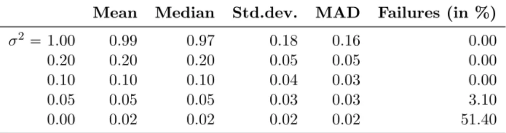
For the Poisson distribution we setσp² 0. Strictly speaking, the log-linear model (3) does not fall into the class of models considered byChristou and Fokianos(2014). However, results obtained byDoucet al.(2013) allow to use this estimator also for the log-linear model (for pq1). This issue is addressed by simulations in Appendix B.2, which support that the estimator obtained by (10) provides good results also for models with the logarithmic link function.

Inference for the regression parameters is based on the asymptotic normality of the QML estimator, which has been shown byFokianos et al.(2009) andChristou and Fokianos (2014) for models without covariates. For a well behaved covariate processtX_tu we conjecture that

?n

θp_nθ₀ ÝÑ^d N_{p q r 1}

0, G_n¹ppθ;σp²qG_nppθqG_n¹ppθ;pσ²q , (11) as nÑ 8, where θ0 denotes the true parameter value and σp² is a consistent estimator of σ². We suppose that this applies under the same assumptions usually made for the ordinary linear regression model (see for example Demidenko 2013, p. 140 ff.). For deterministic covariates these assumptions are ||Xt||   c, i.e., the covariate process is bounded, and lim_nÑ8n¹°_n

t1X_tX^J_t A, where c is a constant and A is a nonsingular matrix. For stochastic covariates it is assumed that the expectationsEpX_tq andE X_tX^J_t

exist and that E X_tX^J_t

is nonsingular. The assumptions imply that the information on each covariate grows linearly with the sample size and that the covariates are not linearly dependent. Fuller(1996, Theorem 9.1.1) shows asymptotic normality of the least squares estimator for a regression model with time series errors under even more general conditions which allow the presence of certain types of trends in the covariates. The asymptotic normality of the QML estimator in our context is supported by the simulations presented in AppendixB.1. A formal proof requires further research. To avoid numerical instabilities when invertingG_nppθ;σp²q we apply

an algorithm which makes use of the fact that it is a real symmetric and positive definite matrix; see AppendixA.3.

An alternative to the normal approximation (11) for obtaining standard errors is a parametric bootstrap procedure, which is part of our package (functionse). Accordingly,B time series are simulated from the model fitted to the original data. The empirical standard errors of the parameter estimates for theseB time series are the bootstrap standard errors. This procedure can compute standard errors not only for the estimated regression parameters but also for the dispersion coefficientpσ².

Implementation

The parameter restrictions which are imposed by the conditionθPΘ can be formulated as d linear inequalities. This means that there exists a matrixU of dimension d pp q r 1q and a vector c of lengthd, such that Θ tθ|U θ ¥cu. For the linear model (2) one needs dp q r 2 constraints to ensure nonnegativity of the latent mean λt and stationarity of the resulting process. For the log-linear model (3) there are neither constraints on the intercept nor on the covariate coefficients and the total number of constraints isd2pp q 1q. In order to enforce strict inequalities the respective constraints are tightened by an arbitrarily small constantξ ¡0; this constant is set to ξ10⁶ by default (argument slackvar).

For solving numerically the maximization problem (9) we employ the functionconstrOptim.

This function applies an algorithm described by Lange(1999, Chapter 14), which essentially enforces the constraints by adding a barrier value to the objective function and then employs an algorithm for unconstrained optimization of this new objective function, iterating these two steps if necessary. By default the quasi-Newton Broyden-Fletcher-Goldfarb-Shanno (BFGS) algorithm is employed for the latter task of unconstrained optimization, which additionally makes use of the score vector (8).

Note that the log-likelihood (7) and the score (8) are conditional on unobserved pre-sample values. They depend on the linear predictor and its partial derivatives, which can be computed recursively using any initialization. We give the recursions and present several strategies for their initialization in AppendixA.1(arguments init.methodand init.drop). Christou and Fokianos(2014, Remark 3.1) show that the effect of the initialization vanishes asymptotically.

Nevertheless, from a practical point of view the initialization of the recursions is crucial.

Especially in the presence of strong serial dependence, the resulting estimates can differ substantially even for long time series with 1000 observations; see the simulated example in Table2 in AppendixA.1.

Solving the non-linear optimization problem (9) requires a starting value for the parameter vector θ. This starting value can be obtained from fitting a simpler model for which an estimation procedure is readily available. We consider either to fit a GLM or to fit an autoregressive moving average (ARMA) model. A third possibility is to fit a naive i.i.d.

model without covariates. As a last choice, note that we could use fixed values which need to be provided by the statistician. All possibilities are available in our package (argument start.control). It turns out that the optimization algorithm converges very reliably even if the starting values are not close to the global optimum of the likelihood. Of course, a starting value closer to the global optimum usually requires fewer iterations until convergence.

However, we have encountered some data examples where starting values close to a local optimum, obtained by one of the first two estimation methods, can even prevent finding the

global optimum. Consequently, we recommend fitting the naive i.i.d. model without covariates to obtain starting values. More details on these approaches are given in AppendixA.2.

4. Prediction

In terms of the mean square error, the optimal predictor Ypn 1 for Yn 1, given potential covariates at time n 1 and the past F_n of the process up to time n, is the conditional expectationλ_{n 1} given in (1). By construction of the model the conditional distribution of Yn 1 is a Poisson (4) respectively Negative Binomial (5) distribution with meanλn 1. Anh-step-ahead prediction Yp_{n h} for Y_{n h} is obtained by recursive one-step-ahead predictions, where unobserved values Y_{n 1}, . . . , Y_{n h1} are replaced by their respective one-step-ahead prediction (S3 method of function predict), h PN. The distribution of this h-step-ahead predictionYp_{n h}is not known analytically but can be approximated numerically by simulation, which is described below.

In applications λn 1 is substituted by its estimator pλn 1 λn 1ppθq, which depends on the estimated model parameters pθ. The dispersion parameter φ of the Negative Binomial distribution is replaced by its estimatorφ. The additional uncertainty induced by plugging inp the estimated model coefficients is not taken into account for the construction of prediction intervals.

Prediction intervals forY_{n h} with a given coverage rate 1α(argument level) are designed to cover the true observation Yn h with a probability of 1α. Simultaneous prediction intervals achieving a global coverage rate forYn 1, . . . , Y_{n h} can be obtained by a Bonferroni adjustment of the individual coverage rates to 1α{heach. The prediction intervals are based onB simulations of realizationsy_n^pbq₁, . . . , y_{n h}^pbq from the fitted model,b1, . . . , B (argument B). To obtain an approximative prediction interval for Y_{n h} one can either use the empirical pα{2q- andp1α{2q-quantile ofy^p_{n h}^1q , . . . , y^p_{n h}^Bq or find the shortest interval which contains at leastrp1αq Bsof these observations (the function predictreturns both types of prediction intervals and additionally the empirical median of the simulated predictive distribution). The computation of prediction intervals can be accelerated by distributing it to multiple cores simultaneously (argumentparallel=TRUE), which requires a computing cluster registered by theRpackage parallel.

5. Model assessment

Tools originally developed for generalized linear models as well as for time series can be utilized to asses the model fit and its predictive performance. Within the class of count time series following generalized linear models it is desirable to asses the specification of the linear predictor as well as the choice of the link function and of the conditional distribution. Note that all tools are introduced as in-sample versions, meaning that the observationsy1. . . , yn are used for fitting the model as well as for assessing the obtained fit. However, it is straightforward to apply such tools as out-of-sample criteria.

Denote the fitted values by pλt λtppθq. Note that these do not depend on the chosen distribution, because the mean is the same regardless of the response distribution. There are

various types of residuals available (S3 method of functionresiduals). Response (or raw) residuals (argumenttype="response") are given by

r_ty_t pλ_t,

whereas a standardized alternative are Pearson residuals (argument type="pearson") r^P_t pyt pλtq{b

pλt pλ²_tσp²,

or the more symmetrically distributed Anscombe residuals (argument type="anscombe") r_t^A 3pσ² 1 y_t{pσ²2{3

1 pλ_t{pσ²2{3

3 y_t^2{3 pλ²_t^{3 2 pλ²_t{pσ² pλt

_1{6 ,

for t 1, . . . , n (see for example Hilbe 2011, Section 5.1). The empirical autocorrelation function of these residuals can demonstrate serial dependence which has not been explained by the fitted model. A plot of the residuals against time can reveal changes of the data generating process over time. Furthermore, a plot of squared residuals r²_t against the corresponding fitted valuesλpt exhibits the relation of mean and variance and might point to the Poisson distribution if the points scatter around the identity function or to the Negative Binomial distribution if there exists a quadratic relation (seeVer Hoef and Boveng 2007).

Christou and Fokianos(2015) extend tools for assessing the predictive performance to count time series, which were originally proposed byGneiting, Balabdaoui, and Raftery(2007) and others for continuous data and transferred to independent but not identically distributed count data byCzado, Gneiting, and Held(2009). These tools follow theprequential principle formulated byDawid (1984), depending only on the realized observations and their respective forecast distributions. Denote byP_tpyq P Y_t¤y|F_t1

the c.d.f., byp_tpyq P Y_ty|F_t1 the p.d.f.,yPN0, and byσtthe standard deviation of the predictive distribution (recall Section4 on one-step-ahead prediction).

A tool for assessing the probabilistic calibration of the predictive distribution (seeGneitinget al.

2007) is theprobability integral transform (PIT), which will follow a uniform distribution if the predictive distribution is correct. For count dataCzadoet al.(2009) define a non-randomized PIT value for the observed valuey_t and the predictive distributionP_tpyq by

F_tpu|yq

$' ''

&

'' '%

0, u¤Ptpy1q

uP_tpy1q

P_tpyq P_tpy1q, P_tpy1q  u P_tpyq

1, u¥Ptpyq

.

The mean PIT is then given by Fpuq 1

n

¸n t1

F_tpu|y_tq, 0¤u¤1.

To check whetherFpuqis the c.d.f. of a uniform distributionCzadoet al.(2009) propose plotting a histogram withHbins, where binhhas the heightfj Fph{HqFpph1q{Hq,h1, . . . , H (functionpit). By default H is chosen to be 10. A U-shape indicates underdispersion of the

predictive distribution, whereas an upside down U-shape indicates overdispersion. Gneiting et al.(2007) point out that the empirical coverage of central, e.g., 90% prediction intervals can be read off the PIT histogram as the area under the 90% central bins.

Marginal calibration is defined as the difference of the average predictive c.d.f. and the empirical c.d.f. of the observations, i.e.,

1 n

¸n t1

Ptpyq 1 n

¸n t1

1pyt¤yq

for ally PR. In practice we plot the marginal calibration for values y in the range of the original observations (Christou and Fokianos 2015) (function marcal). If the predictions from a model are appropriate the marginal distribution of the predictions resembles the marginal distribution of the observations and its plotted difference is close to zero. Major deviations from zero point at model deficiencies.

Gneitinget al.(2007) show that the calibration assessed by a PIT histogram or a marginal calibration plot is a necessary but not sufficient condition for a forecaster to be ideal. They advocate to favor the model with the maximal sharpness among all sufficiently calibrated models. Sharpness is the concentration of the predictive distribution and can be measured by the width of prediction intervals. A simultaneous assessment of calibration and sharpness summarized in a single numerical score can be accomplished byproper scoring rules (Gneiting et al. 2007). Denote a score for the predictive distribution P_t and the observation y_t by spP_t, y_tq. A number of possible proper scoring rules is given in Table 1. The mean score for each corresponding model is given by°_n

t1spPt, ytq{n. The model with the lowest score is preferable. Each of the different proper scoring rules captures different characteristics of the predictive distribution and its distance to the observed data (functionscoring).

Scoring rule Abbreviation Definition logarithmic score logarithmic logpptpytqq quadratic (or Brier) score quadratic 2p_tpy_tq }p_t}²

spherical score spherical ptpytq{ }pt}

ranked probability score rankprob °₈

y0pPtpyq 1pyt¤yqq² Dawid-Sebastiani score dawseb py_tλ_tq²{σ²_t 2 logpσ_tq normalized squared error score normsq pytλtq²{σ_t²

squared error score sqerror pytλtq²

Table 1: Definitions of proper scoring rules spPt, ytq (cf. Czado et al. 2009; Christou and Fokianos 2015) and their abbreviations in the package; }p_t}² °₈

y0p_tpyq².

6. Intervention analysis

In many applications sudden changes or extraordinary events occur. Box and Tiao(1975) refer to such special events as interventions. This could be for example the outbreak of an epidemic in a time series which counts the weekly number of patients infected with a particular disease.

It is of interest to examine the effect of known interventions, for example to judge whether a

policy change had the intended impact, or to search for unknown intervention effects and find explanations for thema posteriori.

Fokianos and Fried (2010, 2012) model interventions affecting the location by including a deterministic covariate of the formδ^tτ1pt¥τq, where τ is the time of occurrence andδ is a known constant (functioninterv_covariate). This covers various types of interventions for different choices of the constantδ: a singular effect forδ0 (spiky outlier), an exponentially decaying change in location forδP p0,1q (transient shift) and a permanent change of location for δ 1 (level shift). Similar to the case of covariates, the effect of an intervention is essentially additive for the linear model and multiplicative for the log-linear model. However, the intervention enters the dynamics of the process and hence its effect on the linear predictor is not purely additive. Our package includes methods to test on such intervention effects developed byFokianos and Fried (2010,2012), suitably adapted to the more general model class described in Section 2. The linear predictor of a model with s types of interventions according to parametersδ1, . . . , δs occurring at time pointsτ1, . . . , τs reads

gpλtq β0

¸p k1

βkgpYr tikq

¸q

`1

α`gpλtj`q η^JXt

¸s m1

ωmδ^t_m^τm1pt¥τmq, (12) where ω₁, . . . , ω_s are the respective intervention sizes. At the time of its occurrence an intervention of sizeω_{`</sub> increases the level of the time series by adding the magnitudeω<sub>`} for a linear model like (2) or by multiplying the factor exppω`qfor a log-linear model like (3). In the following paragraphs we briefly outline the proposed intervention detection procedures and refer to the original articles for details.

Our package allows to test whethers interventions of certain types occurring at given time points according to model (12) have an effect on the observed time series, i.e., to test the hypothesisH0 :ω1 . . .ωs0 against the alternative H1 :ω` 0 for some`P t1, . . . , su, by employing an approximate score test (functioninterv_test). Under the null hypothesis the score test statisticT_npτ₁, . . . , τ_sq has asymptotically a χ²-distribution with sdegrees of freedom, assuming some regularity conditions and for a sufficiently large sample size.

For testing whether a single intervention of a certain type occurring at an unknown time pointτ has an effect, the package employs the maximum of the score test statisticsT_npτq and determines apvalue by a parametric bootstrap procedure (function interv_detect). If we consider a setD of time points at which the intervention might occur, e.g.,D t2, . . . , nu, this test statistic is given byTr_nmax_τPDT_npτq. The bootstrap procedure can be computed on multiple cores simultaneously (argumentparallel=TRUE). The time point of the intervention is estimated to be the valueτ which maximizes this test statistic. Our empirical observation is that such an estimator usually has a large variability. It is possible to speed up the computation of the bootstrap test statistics by using the model parameters used for generation of the bootstrap samples instead of estimating them for each bootstrap sample (argument final.control_bootstrap=NULL). This results in a conservative procedure, as noted by Fokianos and Fried(2012).

If more than one intervention is suspected in the data, but neither their types nor the time points of its occurrences are known, an iterative detection procedure is used (function interv_multiple). Consider the set of possible intervention times Das before and a set of possible intervention types ∆, e.g., ∆ t0,0.8,1u. In a first step the time series is tested for an intervention of each typeδ P∆ as described in the previous paragraph and thepvalues are

Time

Number of cases

1990 1992 1994 1996 1998 2000

01020304050

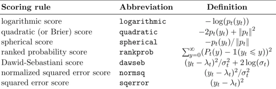
Figure 1: Number of campylobacterosis cases (reported every 28 days) in the north of Qu´ebec in Canada.

Bonferroni-corrected to account for the multiple testing. If none of thep values is below a previously specified significance level, the procedure stops and does not identify an intervention effect. Otherwise the procedure detects an intervention of the type corresponding to the lowest pvalue. In case of equal pvalues preference is given to interventions with δ1, that is level shifts, and then to those with the largest test statistic. In a second step, the effect of the detected intervention is eliminated from the time series and the procedures starts a new step and continues until no further intervention effects are detected. Finally, model (12) with all detected intervention effects can be fitted to the data to estimate the intervention sizes and the other parameters jointly. Note that statistical inference for this final model fit has to be done with care. Further details are given inFokianos and Fried (2010,2012).

Liboschiket al.(2014) study a model for external intervention effects (modeled by external covariate effects, recall (6) and the related discussion) and compare it to internal intervention effects studied in the two aforementioned publications (argumentexternal).

7. Usage of the package

The most recent stable version of thetscount package is distributed via the Comprehensive R Archive Network (CRAN). A current development version is available from the project’s website http://tscount.r-forge.r-project.org on the development platform R-Forge.

After installation of the package it can be loaded inRby typing library("tscount").

The central function for fitting a GLM for count time series is tsglm, whose help page (accessible byhelp(tsglm)) is a good starting point to become familiar with the usage of the

package. We demonstrate typical applications of the package by two data examples.

7.1. Campylobacter infections in Canada

We first analyze the number of campylobacterosis cases (reported every 28 days) in the north of Qu´ebec in Canada shown in Figure 1, which was first reported by Ferland et al. (2006).

These data are made available in our package by the objectcampy. We fit a model to this time

series using the functiontsglm. Following the analysis ofFerlandet al.(2006) we fit model (2) with the identity link function, defined by the argument link. For taking into account serial dependence we include a regression on the previous observation. Seasonality is captured by regressing onλ_t13, the unobserved conditional mean 13 time units (which is one year) back in time. The aforementioned specification of the model for the linear predictor is assigned by the argumentmodel, which has to be a list. We also include the two intervention effects detected by Fokianos and Fried (2010) in the model by suitably chosen covariates provided by the argumentxreg. We compare a fit of a Poisson with that of a Negative Binomial conditional distribution, specified by the argumentdistr. The call for both model fits is then given by:

R> interventions <- interv_covariate(n=length(campy), tau=c(84, 100),

+ delta=c(1, 0))

R> campyfit_pois <- tsglm(campy, model=list(past_obs=1, past_mean=13), + xreg=interventions, dist="poisson")

R> campyfit_nbin <- tsglm(campy, model=list(past_obs=1, past_mean=13), + xreg=interventions, dist="nbinom")

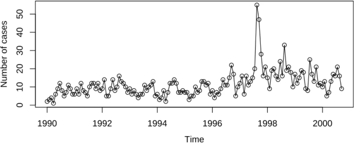
The resulting fitted modelscampyfit_poisandcampyfit_nbinhave class"tsglm", for which a number of methods is provided (see help page), including summary for a detailed model summary andplotfor diagnostic plots. The diagnostic plots in Figure 2are produced by:

R> acf(residuals(campyfit_pois), main="ACF of response residuals")

R> marcal(campyfit_pois, ylim=c(-0.03, 0.03), main="Marginal calibration") R> lines(marcal(campyfit_nbin, plot=FALSE), lty="dashed")

R> legend("bottomright", legend=c("Pois", "NegBin"), lwd=1, + lty=c("solid", "dashed"))

R> pit(campyfit_pois, ylim=c(0, 1.5), main="PIT Poisson")

R> pit(campyfit_nbin, ylim=c(0, 1.5), main="PIT Negative Binomial")

The response residuals are identical for the two conditional distributions. Their empirical autocorrelation function, shown in Figure2top left, does not exhibit remaining serial correlation or seasonality which is not described by the models. The U-shape of the non-randomized PIT histogram in Figure2bottom left indicates that the Poisson distribution does not fully capture this dispersion well, although the U-shape is not very pronounced. As opposed to this, the PIT histogram which corresponds to the Negative Binomial distribution appears to approach uniformity better. Hence the probabilistic calibration of the Negative Binomial model is satisfactory. The marginal calibration plot, shown in Figure2 top right, is inconclusive. As a last tool we consider the scoring rules for the two distributions:

R> rbind(Poisson=scoring(campyfit_pois), NegBin=scoring(campyfit_nbin)) logarithmic quadratic spherical rankprob dawseb

Poisson 2.749861 -0.07669775 -0.2751097 2.199937 3.661858 NegBin 2.721916 -0.07800114 -0.2765980 2.184902 3.605720

normsq sqerror Poisson 1.3075592 16.50839 NegBin 0.9642855 16.50839

0.0 0.5 1.0 1.5

−0.20.20.61.0

Lag

ACF

ACF of response residuals

0 10 20 30 40 50

−0.03−0.010.010.03

Marginal calibration

Threshold value

Diff. of pred. and emp. c.d.f

Pois NegBin

PIT Poisson

Probability integral transform

Density

0.0 0.2 0.4 0.6 0.8 1.0

0.00.51.01.5

PIT Negative Binomial

Probability integral transform

Density

0.0 0.2 0.4 0.6 0.8 1.0

0.00.51.01.5

Figure 2: Diagnostic plots for a fit to the campylobacterosis data.

Two of the scoring rules are slightly in favor of the Poisson distribution (quadratic and spherical score), while the other scoring rules support the Negative Binomial distribution. Based on the the PIT histograms and the results obtained by most of the scoring rules, we decide for a Negative Binomial model. The degree of overdispersion seems to be small, as the estimated overdispersion coefficient’sigmasq’ given in the output below is close to zero.

R> summary(campyfit_nbin) Call:

tsglm(ts = campy, model = list(past_obs = 1, past_mean = 13), xreg = interventions, distr = "nbinom")

Coefficients:

Estimate Std. Error (Intercept) 3.3169 0.7850

beta_1 0.3689 0.0696

alpha_13 0.2201 0.0942

interv_1 3.0864 0.8561

interv_2 41.8628 12.0693

sigmasq 0.0297 NA

Standard errors obtained by normal approximation.

Link function: identity

Distribution family: nbinom (with overdispersion coefficient 'sigmasq') Number of coefficients: 6

Log-likelihood: -381.0682 AIC: 774.1364

BIC: 791.7862

The coefficient beta_1 corresponds to regression on the previous observation, alpha_13 corresponds to regression on values of the latent mean thirteen units back in time. The standard errors of the estimated regression parameters in the summary above are based on the normal approximation given in (11). For the additional overdispersion coefficient sigmasqof the Negative Binomial distribution there is no analytical approximation available for its standard error. Alternatively, standard errors of the regression parameters and the overdispersion coefficient can be obtained by a parametric bootstrap (which takes about 15 minutes computation time on a single 3.2 GHz processor for 500 replications):

R> se(campyfit_nbin, B=500)$se

(Intercept) beta_1 alpha_13 interv_1 interv_2 0.89710834 0.07362390 0.10266237 0.89253577 11.71983693

sigmasq 0.01417654 Warning message:

In se.tsglm(campyfit_nbin, B = 500) :

The overdispersion coefficient 'sigmasq' could not be estimated in 13 of the 500 replications. It is set to zero for these

replications. This might to some extent result in an overestimation of its true variability.

Estimation problems for the dispersion parameter (see warning message) occur occasionally for models where the true overdispersion coefficient σ² is small, i.e., which are close to a Poisson model; see AppendixB.2. The bootstrap standard errors of the regression parameters are slightly larger than those based on the normal approximation. Note that neither of the approaches reflects the additional uncertainty induced by the model selection.

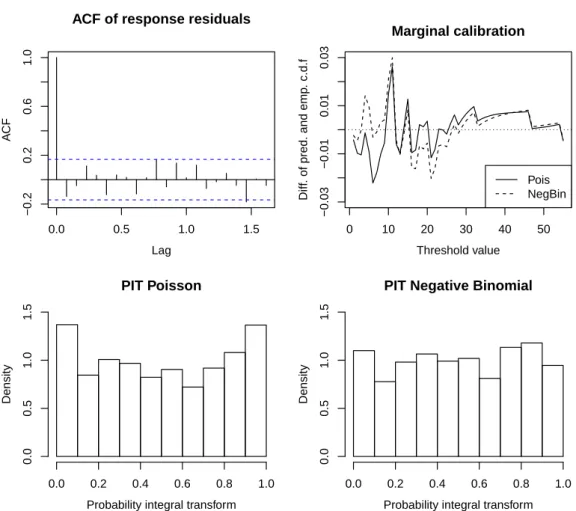
7.2. Road Casualties in Great Britain

Next we study the monthly number of killed drivers of light goods vehicles in Great Britain between January 1969 and December 1984 shown in Figure3. This time series is part of a dataset which was first considered by Harvey and Durbin (1986) for studying the effect of compulsory wearing of seatbelts introduced on 31 January 1983. The dataset, including additional covariates, is available inRin the object Seatbelts. In their paper Harvey and Durbin(1986) analyze the numbers of casualties for drivers and passengers of cars, which are so

Time Number of casualties 51015

1969 1971 1973 1975 1977 1979 1981 1983 1985

Figure 3: Monthly number of killed van drivers in Great Britain. The introduction of compulsory wearing of seatbelts on 31 January 1983 is marked by a vertical line.

large that they can be treated with methods for continuous-valued data in good approximation.

The monthly number of killed drivers of vans analyzed here is much smaller (its minimum is 2 and its maximum 17) and therefore methods for count data are to be preferred.

For model selection we only use the data until December 1981. We choose the log-linear model with the logarithmic link because it allows for negative covariate effects. We try to capture the short range serial dependence by a first order autoregressive term and the yearly seasonality by a 12th order autoregressive term, both declared by the list element named’past_obs’of the argumentmodel. Following Harvey and Durbin(1986) we use the real price of petrol as an explanatory variable. We also include a deterministic covariate describing a linear trend.

Both covariates are provided by the argumentxreg. Based on PIT histograms, a marginal calibration plot and the scoring rules (not shown here) we find that the Poisson distribution is sufficient for modeling. The model is fitted by the call:

R> timeseries <- Seatbelts[, "VanKilled"]

R> regressors <- cbind(PetrolPrice=Seatbelts[, c("PetrolPrice")],

+ linearTrend=seq(along=timeseries)/12)

R> timeseries_until1981 <- window(timeseries, end=1981+11/12) R> regressors_until1981 <- window(regressors, end=1981+11/12) R> seatbeltsfit <- tsglm(ts=timeseries_until1981,

+ model=list(past_obs=c(1, 12)), link="log", distr="pois", + xreg=regressors_until1981)

R> summary(seatbeltsfit, B=500) Call:

tsglm(ts = timeseries_until1981, model = list(past_obs = c(1,

12)), xreg = regressors_until1981, link = "log", distr = "pois") Coefficients:

Estimate Std. Error

(Intercept) 1.8315 0.36817

beta_1 0.0862 0.08194

beta_12 0.1558 0.08782

PetrolPrice 0.7980 2.37008 linearTrend -0.0307 0.00853

Standard errors obtained by parametric bootstrap with 500 replications.

Link function: log

Distribution family: poisson Number of coefficients: 5 Log-likelihood: -396.152 AIC: 802.3039

BIC: 817.5532

The estimated coefficient beta_1corresponding to the first order autocorrelation is very small and even slightly below the size of its approximative standard error, indicating that there is no notable dependence on the number of killed van drivers of the preceding week. We find a seasonal effect captured by the twelfth order autocorrelation coefficientbeta_12. Unlike in the model for the car drivers byHarvey and Durbin (1986), the petrol price does not seem to influence the number of killed van drivers. An explanation might be that vans are much more often used for commercial purposes than cars and that commercial traffic is less influenced by the price of fuel. The linear trend can be interpreted as a yearly reduction of the number of casualties by a factor of 0.97 (obtained by exponentiating the corresponding estimated coefficient), i.e., on average we expect 3% fewer killed van drivers per year (which is below one in absolute numbers).

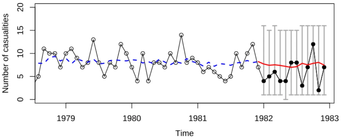
Based on the model fitted to the training data until December 1981, we can predict the number of road casualties in 1982 given the respective petrol price. A graphical representation of the following predictions is given in Figure4.

R> timeseries_1982 <- window(timeseries, start=1982, end=1982+11/12) R> regressors_1982 <- window(regressors, start=1982, end=1982+11/12) R> predict(seatbeltsfit, n.ahead=12, level=1-0.1/12, B=2000,

+ newxreg=regressors_1982)$fit

Jan Feb Mar Apr May Jun Jul

1982 7.702261 7.413734 7.532874 7.382316 7.177786 6.967197 7.129638

Aug Sep Oct Nov Dec

1982 7.844506 7.511275 7.840156 8.049270 7.456153

Finally, we test whether there was an abrupt shift in the number of casualties occurring when the compulsory wearing of seatbelts is introduced on 31 January 1983. The approximative score test described in Section6 is applied:

R> seatbeltsfit_alldata <- tsglm(ts=timeseries, link="log",

+ model=list(past_obs=c(1, 12)),

+ xreg=regressors, distr="pois")

Time

Number of casualities

1979 1980 1981 1982 1983

05101520

Figure 4: Fitted values (blue dashed line) and predicted values (red solid line) according to the model with the Poisson distribution. Prediction intervals (grey bars) are designed to ensure a global coverage rate of 90%. They are chosen to have minimal length and are based on a simulation with 2000 replications.

R> interv_test(seatbeltsfit_alldata, tau=170, delta=1, est_interv=TRUE) Score test on intervention(s) of given type at given time

Chisq-Statistic: 46.80599 on 1 degree(s) of freedom, p-value: 7.837397e-12 Fitted model with the specified intervention:

Call:

tsglm(ts = fit$ts, model = model_extended, xreg = xreg_extended, link = fit$link, distr = fit$distr)

Coefficients:

(Intercept) beta_1 beta_12 PetrolPrice linearTrend

1.93358 0.08185 0.13918 0.41617 -0.03463

interv_1 -0.21696

The null hypothesis of no intervention is rejected at a 5% significance level. The multiplicative effect size of the intervention is found to be 0.805. This indicates that according to this model fit 19.5% less van drivers are killed after the law enforcement. For comparison,Harvey and Durbin(1986) estimate a reduction of 18% for the number of killed car drivers.

8. Outlook

In its current version theR packagetscount allows the analysis of count time series with a quite broad class of models. It will hopefully proof to be useful for a wide range of applications.

Nevertheless, there is a number of desirable extensions of the package which could be included in future releases. We invite other researchers and developers to contribute to this package.

As an alternative to the Negative Binomial distribution, one could consider the so-called Quasi-Poisson distribution. It allows for a conditional variance ofφλ_t (instead ofλ_t φλ²_t, as for the Negative Binomial distribution), which is linearly and not quadratically increasing in the conditional mean λt (for the case of independent data seeVer Hoef and Boveng 2007).

A scatterplot of the squared residuals against the fitted values could reveal whether a linear relation between conditional mean and variance is more adequate for a given time series.

The common regression models for count data are often not capable to describe an exceptionally large number of observations with the value zero. In the literature so-called zero-inflated and hurdle regression models have become popular for zero excess count data (for an introduction and comparison seeLoeys, Moerkerke, De Smet, and Buysse 2012). A first attempt to utilize zero-inflation for INGARCH time series models is made byZhu(2012).

Alternative nonlinear models are for example the threshold model suggested byDouc et al.

(2013) or the examples given by Fokianos and Tjøstheim (2012). Fokianos and Neumann (2013) propose a class of goodness-of-fit tests for the specification of the linear predictor, which are based on the smoothed empirical process of Pearson residuals. Christou and Fokianos (2013) develop suitably adjusted score tests for parameters which are identifiable as well as non-identifiable under the null hypothesis. These tests can be employed to test for linearity of an assumed model.

In practical applications one is often faced with outliers. Elsaied and Fried (2014) and Kitromilidou and Fokianos(2013) develop M-estimators for the linear and the log-linear model respectively. Fried, Liboschik, Elsaied, Kitromilidou, and Fokianos (2014) compare robust estimators of the (partial) autocorrelation for time series of counts, which can be useful for identifying the correct model order.

In the long term, related models for binary or categorical time series (Moysiadis and Fokianos 2014) or potential multivariate extensions of count time series following GLMs could be included as well.

The models which are so far included in the package or mentioned above fall into the class of time series following GLMs. There is also quite a lot of literature on thinning-based time series models but we are not aware of any publicly available software implementations. To name just a few of many publications,Weiß (2008) reviews univariate time series models based on the thinning operation,Pedeli and Karlis(2013) study a multivariate extension and Scotto, Weiß, Silva, and Pereira(2014) consider models for time series with a finite range of counts.

Acknowledgements

Part of this work was done while K. Fokianos was a Gambrinus Fellow at TU Dortmund University. The research of R. Fried and T. Liboschik was supported by the German Research Foundation (DFG, SFB 823 “Statistical modelling of nonlinear dynamic processes”). The authors thank Philipp Probst for his considerable contribution to the development of the package and Jonathan Rathjens for carefully checking the package.

References

Bollerslev T (1986). “Generalized Autoregressive Conditional Heteroskedasticity.”Journal of Econometrics,31(3), 307–327. ISSN 0304-4076. doi:10.1016/0304-4076(86)90063-1.

Box GEP, Tiao GC (1975). “Intervention Analysis with Applications to Economic and Environmental Problems.”Journal of the American Statistical Association, 70(349), 70–79.

ISSN 0162-1459. doi:10.2307/2285379.

Christou V, Fokianos K (2013). “Estimation and Testing Linearity for Mixed Poisson Autore- gressions.” Submitted for publication.

Christou V, Fokianos K (2014). “Quasi-Likelihood Inference for Negative Binomial Time Series Models.” Journal of Time Series Analysis, 35(1), 55–78. ISSN 1467-9892. doi:

10.1111/jtsa.12050.

Christou V, Fokianos K (2015). “On Count Time Series Prediction.” Journal of Statistical Computation and Simulation, 85(2), 357–373. ISSN 0094-9655. doi:10.1080/00949655.

2013.823612.

Czado C, Gneiting T, Held L (2009). “Predictive Model Assessment for Count Data.”Biometrics, 65(4), 1254–1261. ISSN 1541-0420. doi:10.1111/j.1541-0420.2009.01191.x.

Dawid AP (1984). “Statistical Theory: The Prequential Approach.” Journal of the Royal Statistical Society. Series A (General),147(2), 278–292. ISSN 0035-9238. doi:10.2307/

2981683.

Demidenko E (2013). Mixed models: theory and applications with R. Wiley series in probability and statistics, 2nd edition. Wiley, Hoboken. ISBN 978-1-11-809157-9.

Douc R, Doukhan P, Moulines E (2013). “Ergodicity of Observation-Driven Time Series Models and Consistency of the Maximum Likelihood Estimator.” Stochastic Processes and their Applications,123(7), 2620–2647. ISSN 0304-4149. doi:10.1016/j.spa.2013.04.010.

Elsaied H, Fried R (2014). “Robust Fitting of INARCH Models.” Journal of Time Series Analysis,35(6), 517–535. ISSN 1467-9892. doi:10.1111/jtsa.12079.

Fahrmeir L, Tutz G (2001). Multivariate Statistical Modelling Based on Generalized Linear Models. Springer, New York. ISBN 9780387951874.

Ferland R, Latour A, Oraichi D (2006). “Integer-Valued GARCH Process.”Journal of Time Series Analysis,27(6), 923–942. ISSN 1467-9892. doi:10.1111/j.1467-9892.2006.00496.

x.

Fokianos K (2011). “Some Recent Progress in Count Time Series.” Statistics: A Journal of Theoretical and Applied Statistics,45(1), 49. ISSN 0233-1888. doi:10.1080/02331888.

2010.541250.

Fokianos K (2012). “Count Time Series Models.” In T Subba Rao, S Subba Rao, C Rao (eds.), Time Series – Methods and Applications, number 30 in Handbook of Statistics, pp. 315–347.

Elsevier, Amsterdam. ISBN 978-0-444-53858-1.

Fokianos K (2015). “Statistical Analysis of Count Time Series Models.” In R Davis, S Holan, R Lund, N Ravishanker (eds.), Handbook of Discrete-Valued Time Series, Handbooks of Modern Statistical Methods. Chapman & Hall, London. To appear.

Fokianos K, Fried R (2010). “Interventions in INGARCH Processes.”Journal of Time Series Analysis,31(3), 210–225. ISSN 01439782. doi:10.1111/j.1467-9892.2010.00657.x.

Fokianos K, Fried R (2012). “Interventions in Log-Linear Poisson Autoregression.”

Statistical Modelling, 12(4), 299–322. ISSN 1471-082X, 1477-0342. doi:10.1177/

1471082X1201200401.

Fokianos K, Neumann MH (2013). “A Goodness-Of-Fit Test for Poisson Count Processes.”

Electronic Journal of Statistics,7, 793–819. ISSN 1935-7524. doi:10.1214/13-EJS790.

Fokianos K, Rahbek A, Tjøstheim D (2009). “Poisson Autoregression.”Journal of the American Statistical Association, 104(488), 1430–1439. ISSN 0162-1459. doi:10.1198/jasa.2009.

tm08270.

Fokianos K, Tjøstheim D (2011). “Log-Linear Poisson Autoregression.”Journal of Multivariate Analysis,102(3), 563–578. ISSN 0047-259X. doi:10.1016/j.jmva.2010.11.002.

Fokianos K, Tjøstheim D (2012). “Nonlinear Poisson Autoregression.”Annals of the Institute of Statistical Mathematics,64(6), 1205–1225. ISSN 0020-3157, 1572-9052. doi:10.1007/

s10463-012-0351-3.

Fried R, Liboschik T, Elsaied H, Kitromilidou S, Fokianos K (2014). “On Outliers and Interventions in Count Time Series Following GLMs.”Austrian Journal of Statistics, 43(3), 181–193. ISSN 1026-597X. URLhttp://www.ajs.or.at/index.php/ajs/article/view/

vol43-3-2.

Fuller WA (1996). Introduction to Statistical Time Series. 2nd edition. Wiley, New York.

ISBN 0-471-55239-9.

Gneiting T, Balabdaoui F, Raftery AE (2007). “Probabilistic Forecasts, Calibration and Sharpness.” Journal of the Royal Statistical Society: Series B (Statistical Methodology), 69(2), 243–268. ISSN 1467-9868. doi:10.1111/j.1467-9868.2007.00587.x.

Harvey AC, Durbin J (1986). “The Effects of Seat Belt Legislation on British Road Casualties:

A Case Study in Structural Time Series Modelling.” Journal of the Royal Statistical Society.

Series A (General),149(3), 187–227. ISSN 0035-9238. doi:10.2307/2981553.

Heinen A (2003). “Modelling Time Series Count Data: An Autoregressive Conditional Poisson Model.”CORE discussion paper,62. doi:10.2139/ssrn.1117187.

Hilbe JM (2011). Negative Binomial Regression. 2nd edition. Cambridge University Press, Cambridge. ISBN 9780521198158.

Jung R, Tremayne A (2011). “Useful Models for Time Series of Counts or Simply Wrong Ones?” AStA Advances in Statistical Analysis, 95(1), 59–91. ISSN 1863-8171. doi:

10.1007/s10182-010-0139-9.