Application of Non-Linear Time Series Models to Power Risk Management: A Case Study for Germany

Application of Non-Linear Time Series Models to Power Risk Management:

A Case Study for Germany Inauguraldissertation

zur

Erlangung des Doktogrades der

Wirtschafts- und Sozialwissenschaftlichen Fakult¨at der

Universit¨at zu K¨oln 2007

vorgelegt von

Diplom-Volkswirt Peter Kosater aus

Berent/Polen

Referent: Prof. Dr. Karl Mosler

Korreferent: Prof. Dr. Eckart Bomsdorf

Tag der Promotion: 9.02.07

Vorwort

Diese Arbeit ist das Ergebnis eines Projektes im Rahmen des Graduiertenkollegs Risikomanagement an der Universit¨at zu K¨oln, an dem ich das Gl¨ uck hatte, in den Jahren 2003 bis 2006 teilnehmen zu d¨ urfen.

Wie im t¨aglichen Leben allgemein w¨are diese Arbeit nicht ohne die Hilfe anderer zustandegekommen. Als erste und wichtigste Bezugsperson m¨ochte ich meinen Doktorvater Prof.Dr.Karl Mosler danken f¨ ur die fachliche und finanzielle Un- terst¨ utzung als auch insbesondere die kritischen Kommentare zu den Arbeitspa- pieren, die im Verlauf der Dissertation entstanden sind.

Weiterhin danke ich Prof.Dr.Alexander Kempf stellvertretend f¨ ur die das

Graduiertenkolleg tragenden Professoren sowie die DFG, die in einer gemeinsamen Kraftanstrengung das Graduiertenkolleg aus der Taufe gehoben haben. Im Rah- men der Promotion innerhalb des Kollegs habe ich inhaltliche und pers¨onliche Qualifikationen erworben, die mir auch im beruflichen Alltag nach Abschluss der Promotion hilfreich sind, obwohl ich selbst w¨ahrend der Promotionsphase nicht daran geglaubt hatte.

Schließlich m¨ochte ich noch Prof.Dr.Eckart Bomsdorf f¨ ur die ¨ Ubernahme des Kor- referats und die kritischen Kommentare sowie Prof.Dr.Dieter Hess f¨ ur die ¨ Ubernahme des Vorsitzes bei meiner Disputation danken.

Ferner m¨ochte ich meinen Kollegen aus den verschiedenen Kohorten danken. Beson- ders erw¨ahnt seien Daniel Mayston f¨ ur die Nachhilfe im Verfassen englischsprachiger Zeitschriftenartikel sowie Martin Honal und Tanja Thiele f¨ ur viele Gespr¨ache, die geholfen haben ¨ uber die vielen Selbstzweifel w¨ahrend der Arbeit hinwegzukom- men. Den Teilnehmern des Oberseminars der beiden Statistiklehrst¨ uhle danke ich f¨ ur die hilfreichen Kommentare.

Eine gute Promotion ist offen f¨ ur Impulse von außerhalb. Deshalb m¨ochte ich stellvertretend vor allem Dr. Cyriel de Jong von der Erasmus Universit¨at in Rot- terdam f¨ ur seine Hilfe danken. Bedankt voor jouw hulp, Cyriel. Hoe je ziet, ik heb nu toch een beetje Nederlands geleerd.

Eine Promotion wirkt sich bis in den privaten Bereich aus. Deshalb m¨ochte ich im speziellen Anna Cellarova f¨ ur Ihren seelischen Beistand danken. ˇ Dakujem ti a prajem ti ˇ vsetko najlepˇ sie.

Abschliessend m¨ochte ich meiner Familie und da vor allem meiner Mutter f¨ ur die

Unterst¨ utzung danken.

Abstract

As a consequence of the ongoing liberalization process, sensible management in the electricity sector has to take into account the market price risk as well as volume risks.

Market price risk mainly arises due to the scarce storability of electricity which causes spot prices to be highly volatile. Secondly, the demand for electricity strongly depends on weather conditions. Electricity suppliers sell less power dur- ing mild winters than expected beforehand. Consequently, the suppliers are faced with volume risks.

To cope with the market price risk suitable models of the spot price are required.

These models can be exploited for pricing of derivatives on the electricity spot price as the underlying on one hand and the short term optimization of the pro- duction schedule on the other hand.

In the first part of the thesis, the author discusses some of the existing approaches to the modelling of spot prices and puts forward a new approach. In addition, he examines the impact of weather on electricity spot prices.

In the second part of the thesis, the author discusses bivariate modelling of temper- ature time series which is crucial for cross-city hedging with weather derivatives.

Weather derivatives are financial instruments which allow to hedge against volume risks emerging from unforeseen weather conditions.

Zusammenfassung

Die Liberalisierung des Energiesektors stellt Energiemanager vor neue Aufgaben.

Sie m¨ ussen sich mit Marktpreis- und Mengenrisiken auseinandersetzen.

Marktpreisrisiken spiegeln sich in der hohen Volatilit¨at der Spotpreise wider, die haupts¨achlich in der Nichtspeicherbarkeit von Strom begr¨ undet ist. Ferner ist die Nachfrage nach Strom stark wetterabh¨angig. W¨ahrend milder Winter wird weniger Strom abgesetzt als erwartet. Folglich sind Stromproduzenten auch einem Men- genrisiko ausgesetzt.

Um sich gegen Marktpreisrisiken abzusichern, sind geeignete Modelle f¨ ur den Spotpreis notwendig. Diese Modelle k¨onnen zur Bewertung von Derivaten auf dem Spotpreis als dem Underlying einerseits und zur operationalen Kurzfristopti- mierung andererseits eingesetzt werden.

Im ersten Teil der Arbeit diskutiert der Verfasser ausgew¨ahlte bestehende Ans¨atze zur Spotpreismodellierung und stellt einen neuen Ansatz vor. Außerdem unter- sucht der Verfasser den Einfluss von Wetter auf die Spotpreise.

Im zweiten Teil der Arbeit, wird die Bivariate Modellierung von Temperaturzeitrei-

hen diskutiert. Dies ist von Bedeutung f¨ ur Cross- city hedging mit Wetter-

derivaten. Wetterderivate sind Finanzinstrumente, die es erlauben sich gegen

Mengenrisiken hervorgerufen durch unvorhergesehene Wetterbedingungen abzu-

sichern.

Contents

1 Introduction 11

2 Markov Regime-Switching Models for Electricity Spot Prices 14

2.1 Review of Literature on Electricity Spot Prices . . . . 14

2.2 Data and Descriptive Statistics . . . . 16

2.3 Stochastic Models for Power Prices . . . . 20

2.3.1 AR(1) Process with Drift . . . . 20

2.3.2 The Jump Model . . . . 20

2.3.3 A Markov Regime-Switching Model for Spot Prices: Ethier and Mount(1998) . . . . 22

2.3.4 Two-Regime Model with Independent Spikes : De Jong and Huisman (2003) . . . . 23

2.3.5 Estimation of Markov Regime-Switching Models . . . . 24

2.3.6 Regime-Switching Models with Day-Dependent Spikes: Kosater and Mosler (2006) . . . . 26

2.4 A Forecast Comparison Study . . . . 31

2.4.1 Theoretical Preliminaries . . . . 32

2.4.2 Results of the Study . . . . 34

2.5 Regime-Switching Models and GARCH . . . . 38

2.5.1 Two-Regime Switching Model with GARCH(1,1) Errors . . 40

2.5.2 Two-Regime- Switching Model with ARCH(1) Errors . . . 42

2.5.3 Two-Regime-Switching Model with Independent Spikes and ARCH(1) Errors . . . . 42

2.6 Summary . . . . 46

3 The Impact of Weather on German Hourly Electricity Prices 47 3.1 Introduction . . . . 47

3.2 Data and Descriptive statistics . . . . 48

3.3 Choice of the Weather Variables . . . . 55

3.4 The Empirical Study . . . . 57

3.4.1 Results on Model Fit . . . . 58

3.4.2 A Forecasting Experiment . . . . 71

3.4.3 Results of the Forecasting Study . . . . 72

3.4.4 An Additional Small Forecasting Study . . . . 76

3.5 Summary . . . . 78

4 Cross-City Hedging with Weather Derivatives using Bivariate GARCH Models with Dynamic Conditional Correlations 80

4.1 Introduction and Literature Review . . . . 80

4.2 Data . . . . 84

4.3 Univariate Modelling . . . . 87

4.3.1 Results on Model Fit . . . . 91

4.3.2 Examining the Departure from Normality . . . . 96

4.3.3 Out-of-sample Forecasting Study . . . . 97

4.4 Bivariate Modelling . . . 101

4.4.1 The DCC Model Class . . . 102

4.4.2 Flexible Dynamic Correlations models . . . 104

4.4.3 Two-Step Estimation Procedure . . . 104

4.4.4 Results on Model fit . . . 105

4.5 Forecasting Conditional Correlations . . . 113

4.5.1 Forecasting Correlations in Asymmetric DCC Models . . . 113

4.5.2 Forecasting Correlations in the Flexible Dynamic Correla- tion Models. . . 114

4.6 Cross-City Hedging . . . 119

4.7 Summary . . . 120

5 Conclusion 122

List of Figures

2.2.1 Plots for baseload spot prices, the logarithm of baseload spot prices, log(baseload), and the traded volume at the EEX. . . . 18 2.2.2 Quantile-quantile plots for baseload spot prices at the EEX. . . . . 19 2.2.3 Weekly seasonality of baseload spot prices at the EEX. . . . 19 2.3.1 Plots showing smoothed spike regime probabilities for the following

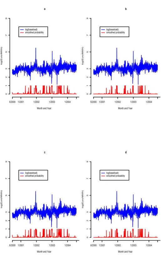
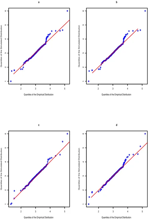
models: (a) Ethier and Mount (1998), (b) De Jong and Huisman (2003), (c) Kosater and Mosler (2006)(without independent spikes), (d) Kosater and Mosler (2006) (with independent spikes). . . . 29 2.3.2 Quantile-quantile plots for log(baseload) from which the determin-

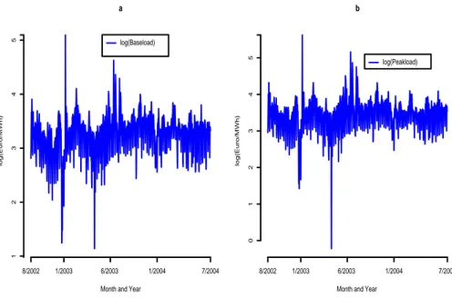
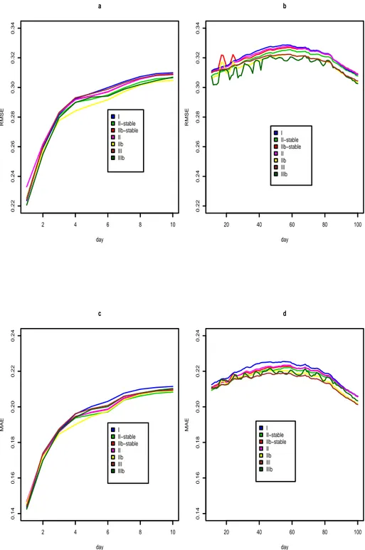
istic effects have been removed against the estimated models: (a) Ethier and Mount (1998), (b) De Jong and Huisman (2003), (c) Kosater and Mosler (2006)(without independent spikes), (d) Kosater and Mosler (2006) (with independent spikes), (Note: To guarantee comparability, two elements in each simulated series throughout the four plots are set equal to 1 and 6, respectively ). . . . 30 2.3.3 Forecast horizon : 25 ^th August 2002 to 28 ^th July 2004. . . . . 31 2.4.1 Results of all models for the log(baseload) time series ( RMSE means

root mean square error and MAE means mean absolute error). . . 36 2.4.2 Results of all models for the log(peakload) time series ( RMSE

means root mean square error and MAE means mean absolute error). 37 2.5.1 Histograms for log(baseload) from which the deterministic effects

have been removed are plotted together with the estimated normal probability densities for the models I to IIIb, according to section 2.4. 39 2.5.2 Smoothed probabilities for the spike regime and quantile-quantile

plots for log(baseload) from which the deterministic effects have been removed against the estimated models: ((a),(b)) MS Model with GARCH(1,1), ((c)(d)) Two-Regime Model with ARCH(1), ((e)(f)) Two- Regime Model with Independent Spikes and ARCH(1), (Note: To guarantee comparability, two elements in each simulated series throughout the three quantile-quantile plots (b,d,f) are set equal to -0.1 and 5, respectively). . . . . 45 3.2.1 (a) Hourly power price series of the EEX, (b) Measured hourly wind

velocity of Holzdorf, (c) Measured hourly temperature of Ulm, (d)

Boxplot for hourly wind velocities, all data ranges from June 16 ^th

2000 to December 31 ^th 2004. . . . 51

3.2.2 Scatter plots for hourly temperature from Ulm and the hourly av- erage wind velocity of Holzdorf and Hamburg with the logarithm of the hourly price series (a,b), one day-ahead forecasts for tempera- ture from Ulm and for wind velocity from Holzdorf (c,d), for 7 a.m.

1/05/2005 until 6 a.m. 1/06/2005, Correlation of measured tem- perature from Ulm and wind velocity from Holzdorf as well as its one day-ahead forecasts with the hourly price for 7 a.m. 1/05/2005 until 6 a.m. 1/06/2005 (e,f). . . . 54 3.3.1 Coefficients of determination R ² : (a) equation (3.3.1), (b) equa-

tion (3.3.2), (c) equation (3.3.3), (d) equation (3.3.4), (e) equation (3.3.2) for the average of three or four stations, (f) equation (3.3.4) for the average of three or four stations. . . . 56 3.4.1 Measured temperature from Ulm (a),(c) and measured wind veloc-

ity (b),(d) together with their two and three days ahead forecasts from hour 7 a.m. 1/05/2005 until hour 6 a.m. 1/06/2005. . . . 73 3.4.2 Results of the forecasting study (a,b), (c,d) R ² of equations (3.4.9)

and (3.4.10). . . . 75 4.2.1 Daily average temperature from Echterdingen( 01/01/1991 until

04/29/2005 (a), Histogram for Echterdingen (b), Autocorrelation function ( ACF ) for Echterdingen (c), Partial autocorrelation func- tion ( PACF )for Echterdingen (d). . . . 86 4.3.1 ACF of the residuals from equation(4.3.9) (a), PACF of the residuals

from equation(4.3.9) (b), ACF of the squared residuals from equa- tion(4.3.9) (c), PACF of the squared residuals from equation(4.3.9)(d), plot of the standardised squared residuals from equation (4.3.9)(e), histogram of the residuals from equation(4.3.9)(f). . . . 90 4.3.2 σ ² _t : Model III (a), σ _t ² : Model IV (b), h t : Model III (c), h t : Model

IV (d), all series for Echterdingen. . . . 95 4.3.3 h _t : Model III and IIIb (a), h _t : Model III and Model IV (b),h _t :

Model IV and IVb (c), h t : Model IIIb and Model IVb (d), all series for Echterdingen. . . . 99 4.4.1 Conditional correlations estimated by QML: DCC and Asymmetric

DCC Echterdingen-Berlin (a),FDC Echterdingen-Berlin (b), DCC and Asymmetric DCC Hamburg-Berlin (c), FDC Hamburg-Berlin (d). . . 112 4.5.1 Point and interval forecasts ( 99 %) for the HDD period 11/01/2004

until 03/31/2005 for Hamburg from : the symmetric DCC (a), the asymmetric DCC (b), FDC of Christodoulakis and Satchell (2002) (c), FDC of Baur (2006) (d), FDC of Kosater (2006)(e). . . 116 4.5.2 Point forecasts of the conditional correlations for the HDD period

11/01/2004 until 03/31/2005 for Echterdingen-Berlin from : the

symmetric DCC (Forecast Q correponds to equation (4.5.2) and

Forecast R corresponds to equation (4.5.3) )(a), the asymmetric

DCC (b), FDC of Christodoulakis and Satchell (2002) (c), FDC of

Baur (2006) (d), FDC of Kosater (2006)(e). . . 117

4.5.3 Point forecasts of conditional correlations for the HDD period 11/01/2004

to 03/31/2005 for Hamburg-Berlin from : the symmetric DCC

(Forecast Q correponds to equation (4.5.2) and Forecast R corre-

sponds to equation (4.5.3) )(a), the asymmetric DCC (b), FDC of

Christodoulakis and Satchell (2002) (c), FDC of Baur (2006) (d),

FDC of Kosater (2006)(e). . . 118

List of Tables

2.2.1 Descriptive Statistics on Baseload and Peakload in Euro/MWh. . . 16 2.3.1 Results on the AR(1) Model, equation(2.3.1), and the Jump Model,

equation (2.3.2). . . . . 21 2.3.2 Results on the Two-Regime Switching Models, see equations (2.3.4-

2.3.8). . . . 24 2.3.3 Results on Two- Regime Models with Day-Dependent Spikes, see

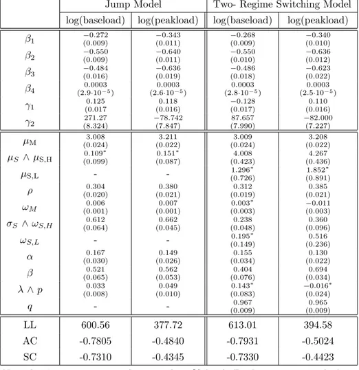
equations (2.3.17-2.3.21). . . . 28 2.5.1 Results on the Jump Model and the Two-Regime Switching Model

with GARCH(1,1) Errors, see equations(2.5.1-2.5.7). . . . 41 2.5.2 Results on Two-Regime Models with ARCH(1) errors, see equations

(2.5.8-2.5.21). . . . 44 3.2.1 Descriptive Statistics on Hourly Spot Prices at the EEX in Euro/MWh. 52 3.2.2 Descriptive Statistics on Temperature in C ^◦ . . . . 53 3.2.3 Descriptive Statistics on Wind Velocity in meter/second. . . . 53 3.4.1 Results on the Stochastic Component and Model Selection Criteria.

(I) . . . . 60 3.4.2 Results on the Stochastic Component and Model Selection Criteria

(II). . . . 61 3.4.3 Summary in-sample fit and the Schwartz Criterion (SC) for all 24

hours. . . . 62 3.4.4 Results on the Deterministic Component, see equation (3.4.2), (I). 63 3.4.5 Results on the Deterministic Component, see equation (3.4.2), (II). 64 3.4.6 Results on the Deterministic Component, see equation (3.4.2), (III). 65 3.4.7 Results on the Deterministic Component, see equation (3.4.2), (IV). 66 3.4.8 Results on the Weather Component w t , see equation (3.4.3) . . . . 67 3.4.9 Results on Constant Transition Probabilities, see equation(3.4.4) . 68 3.4.10 Summary of results for the time-varying transition probabilities

(I), see equation (3.4.4) . . . . 69 3.4.11 Summary of results for the time-varying transition probabilities

(II), see equation (3.4.4) . . . . 70 3.4.12 Summary Out-Of-Sample Forecasting Study. (Best results are

emphasized in bold.) . . . . 74 3.4.13 RMSE for The Three Selected Hours.( Best results are empha-

sized in bold.) . . . . 77 3.4.14 MAE for The Three Selected Hours.( Best results are emphasized

in bold.) . . . . 78

3.4.15 RMSE for The Three Selected Hours.( Best results are empha-

sized in bold.) . . . . 78

3.4.16 MAE for The Three Selected Hours. ( Best results are emphasized in bold.) . . . . 79

4.2.1 Descriptive Statistics on Temperature Series in C ^◦ from The Three Selected Stations. . . . 85

4.2.2 Correlations of Temperature Series in C ^◦ from The Three Selected Stations. . . . 87

4.3.1 Summary In-Sample Fit : Echterdingen. . . . 91

4.3.2 Summary In-Sample Fit : Berlin. . . . 92

4.3.3 Summary In-Sample Fit : Hamburg. . . . 92

4.3.4 Estimates of Models I and II (equations (4.3.9),(4.3.10) and (4.3.13)). 93 4.3.5 Estimates of Models III and IV, (equations (4.3.14) and (4.3.15)). . 94

4.3.6 Summary In-Sample Fit: Model IIIb. . . . 97

4.3.7 Summary In-Sample Fit: Model IVb. . . . 97

4.3.8 Results on The Out-Of-Sample Forecasting Study.( Best results are emphasized in bold.) . . . 101

4.4.1 Summary In-Sample Fit : DCC Models by Engle (2002) and Capiello et al. (2003), ( Two- step estimation ). . . 107

4.4.2 Summary In-Sample Fit : DCC Models by Engle (2002) and Capiello et al. (2003), ( Two- step estimation ). . . 107

4.4.3 Summary In-Sample Fit: DCC Models by Engle (2002) and Capiello et al. (2003), ( QML ). . . 107

4.4.4 Summary In-Sample Fit: DCC Models by Engle (2002) and Capiello et al. (2003), ( QML ). . . 108

4.4.5 Summary In-Sample Fit : Satchell and Christodoulakis (2002), equation(4.4.11). . . 108

4.4.6 Summary In-Sample Fit : Satchell and Christodoulakis (2002), equation(4.4.11). . . 109

4.4.7 Summary In-Sample Fit : Baur (2006), equation(4.4.12). . . . 109

4.4.8 Summary In-Sample Fit : Baur (2006), equation(4.4.12). . . . 110

4.4.9 Summary In-Sample Fit : Kosater (2006), equation(4.4.13). . . . 110

4.4.10 Summary In-Sample Fit : Kosater (2006), equation(4.4.13). . . 111

Chapter 1

Introduction

Until recently, the electricity sector has been a vertically integrated industry and prices have been fixed by regulators. The rapidly progressing deregulation is now leading to gradually privatised electricity markets. These markets divide into for- ward markets, on one hand, and spot markets on the other hand. Especially in spot markets, market participants are exposed to very volatile prices and high un- certainty. Since storability of electricity is limited, spot and forward prices cannot be easily linked. Consequently, forward and spot prices require a separate analysis.

In this thesis, we focus on electricity spot markets, since spot prices are more chal- lenging in modelling than forward prices. Our empirical investigations focus on the spot market at the European Energy Exchange in Leipzig.

As in the commodity and financial markets, derivatives can be used to cope with the large uncertainty due to highly volatile prices. However, pricing of derivatives with the spot price as the underlying asset has to take into account the salient characteristics of electricity spot prices. These features are several seasonality cy- cles, mean reversion and extreme price spikes. Spikes are a direct consequence of the non-storable nature of electricity and are usually explained either by unex- pected outages of large power plants or unpredicted changes of weather conditions.

In most cases, spikes are very short-lived but they can also last for several days in a row.

Besides derivative pricing, short-term price forecasting is of crucial interest for spot market participants. Since spot prices are typically determined through an auction, market participants are requested to express their bids in terms of prices and quantities. Consequently, market participants who are able to accurately fore- cast spot prices can adjust their production schedule to maximize their profits.

Derivative pricing as well as short-term price forecasting require a suitable spot price model. Time series models are capable of capturing the salient characteristics of electricity prices. However, spikes induce non-linearities into the price process.

Therefore, we especially focus on non-linear time series approaches. Among sev-

eral non-linear time series approaches, we opt for Markov regime-switching models

in spirit to Hamilton (1989). Markov regime-switching models are tailor-made for

spot prices and very flexible in modelling non-linearities. In addition, forecasting

can be easily carried out following Hamilton (1989).

The second chapter is dedicated to the application of Markov regime-switching models to spot prices. More precisely, we start with a discussion and application of two established Markov regime-switching models. In a second step, we extend these models by introducing day-dependent spikes. With the inclusion of day- dependent spikes, we take into account that large sized upward spikes are not to be expected on days such as weekends or holidays when demand is usually low.

In a forecasting study, we show that our model extensions do not only successfully capture main characteristics of electricity prices but are also an asset in terms of forecasting.

We conclude with a presentation of model extensions of the models with day- dependent spikes which take into account autoregressive conditional heteroscedas- ticity dynamics.

Hence, the contribution to the literature in the first part of the thesis is the intro- duction of new models which are an asset in derivative pricing and forecasting.

In the third chapter, the relation between weather, represented by temperature and wind velocity, and hourly electricity prices from the European Energy Ex- change in Leipzig is investigated. Furthermore, we assess whether the relation between weather and prices can be successfully exploited for short-term forecast- ing. Thereby, we proceed in the framework of a Markov regime-switching model with day-dependent spikes.

The additional input to existing literature is the examination of the relationship between temperature and wind, on one hand, and hourly power prices from the EEX on the other. Moreover, we prove that transition probabilities, which govern the transition between the regimes, can be successfully modelled as functions of temperature and wind velocity for a couple of hours. Finally, we assess the signif- icance of the relation between weather variables and hourly prices for forecasting hourly prices at the EEX.

As monopolies gave their way to competitive wholesale electricity markets, volu- metric risk came into play. Therefore in the fourth chapter, we turn to a discus- sion of weather derivatives which can be bought by electricity suppliers to protect from revenue uncertainties due to unexpected weather conditions. Our focus is on temperature derivatives. Yet, exchange-based trading of temperature deriva- tives mainly takes place at the Chicago Mercantile Exchange. Since temperature contracts at the Chicago Mercantile Exchange can only be struck for weather vari- ables measured at few selected locations, electricity supplier who wish to hedge their risk at non-traded locations have to correlate their risk with the risk at trade- able locations.

We examine the usefulness of bivariate GARCH models with dynamic conditional correlations in modelling the correlation between non-traded and traded temper- ature time series.

The knowledge of correlation dynamics between these temperature time series en- ables an electricity supplier to correlate his risk with the risk of a traded city and to construct a sensible hedge.

The contribution to the existing literature can be described as follows. We extend

the existing univariate GARCH framework for temperature time series to the bi- variate case. Bivariate GARCH models allow us to explicitly address and model conditional correlation dynamics between two temperature time series. Knowing the conditional correlation dynamics is the key to construct a cross-city hedge.

In chapter five, we summarize our work and highlight the contributions of these

thesis. Finally, we outline hints for further research.

Chapter 2

Markov Regime-Switching Models for Electricity Spot Prices

2.1 Review of Literature on Electricity Spot Prices

To highlight the contribution to the literature made in this chapter, we have to summarize previous work, first. Here, we especially outline important articles on electricity spot prices. However, we also mention parts of our own work which have already been evaluated and quoted by other authors in the meantime.

To start with, important initial articles are those of Knittel and Roberts (2005) and of Lucia and Schwartz (2002). Knittel and Roberts (2005) evaluate the forecast performance of several univariate models using Californian power prices. More- over, they successfully include temperature as covariate. Lucia and Schwartz (2002) present analytic formulas for the pricing of power derivatives. In addition, they take seasonality and mean reversion into account. Escribano et al. (2002) suggest a very general jump model approach. They incorporate mean reversion, spikes and generalized autoregressive conditional heteroscedasticity (GARCH) in their approach for the modelling of electricity spot prices. Moreover, Cuaresma et al.(2004) carry out a forecast study with several linear univariate time series models. They use data from the European Energy Exchange ( EEX )in Germany.

Angeles et al., forthcoming in (2007), provide empirical evidence of periodic ex-

tensions of regression models with autoregressive fractionally integrated moving

average disturbances for the analysis of daily spot prices. They apply their mod-

els to four different markets. Burger et al. (2004) derive a spot market model for

hourly power prices at the EEX. They base their model on economic fundamentals

of power prices in combination with a seasonal autoregressive integrated moving

average approach. Rambharat et al. (2005) propose a threshold autoregressive

model for daily spot prices from Pennsylvania. They incorporate a flexible mean

reversion rate depending on temperature and spikes. More recently, Misioreket

al. (2006) found that threshold autoregressive regime-switching models clearly

outperformed linear approaches in terms of interval forecasts for data from the

California Power Exchange.

Basic idea behind non-linear Markov regime-switching approaches in spirit to Hamilton (1989) is to model spikes as a separate regime. Modelling approaches based on regime-switching have been suggested and successfully applied for in- stance by Ethier and Mount (1998), Huisman and Mahieu (2003), De Jong and Huisman (2003), Kosater and Mosler (2006). The latter focussed on the fore- casting ability of Markov regime-switching models, whereas the remaining authors stressed applicability in derivative pricing. In addition, Mount et al. (2006) show that daily price spikes in the Pennsylvania-New Jersey-Maryland (PJM) Power Pool can be very accurately predicted one day-ahead if load and the reserve mar- gin are included in the model specification and transition probabilities are modelled as functions of load and the reserve margin. Finally, De Jong (2006) tests several spot price models on day-ahead markets in Europe and the USA. The author finds that regime-switching models outperform GARCH(1,1) and Poisson jump models.

Furthermore, De Jong argues that especially regime-switching models with day- dependent spikes as suggested by Kosater and Mosler (2006) are very well suited to capture dynamics in many markets.

In the remainder of the chapter, we discuss and apply selected spot price models

to data from the EEX. In addition, we assess the out-of-sample forecast ability

of some selected Markov regime-switching models. Finally, we give an outlook on

further research.

2.2 Data and Descriptive Statistics

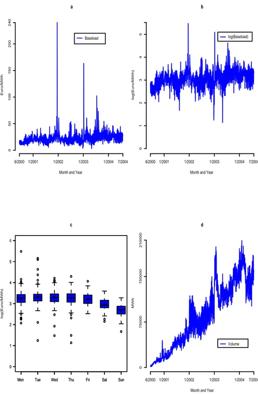
The European Energy Exchange (EEX) in Leipzig is the largest national power exchange in Europe. EEX wholesale electricity prices for 24 hours of the follow- ing day are determined through an auction. These day-ahead prices are typically referred to as spot prices. Besides hourly prices, so-called baseload and peak- load prices are traded. The exchange EEX defines baseload prices as an equally weighted average of the 24 individual hourly prices, while peakload prices are determined by the equally weighted average of prices from 9 am to 8 pm. For our investigations on baseload and peakload, we use data including baseload and peakload price series which range from June 16 ^th 2000 to July 28 ^th 2004. Figure 2.2.1 shows the baseload series that exhibits typical features of power prices like mean reversion and spikes. Table 2.2.1 presents some descriptive statistics for the baseload and peakload series given in Euro/MWh, respectively. Obviously, the descriptive statistics tell us that daily average spot prices are far from being nor- mally distributed. Spot prices tend to fluctuate around a long term equilibrium.

Table 2.2.1: Descriptive Statistics on Baseload and Peakload in Euro/MWh.

Baseload Peakload

Mean 24.77 30.84

Median 23.62 28.53

Maximum 240.26 445.09

Minimum 3.12 0.80

Std. Dev. 11.872 19.302 Skewness 6.908 10.059 Kurtosis 103.82 180.00

This fluctuation is due to shifts in demand caused by weather, for example. Thus, the expression mean reversion describes the tendency of spot prices to revert to a long term equilibrium. Let P t with time-index t ∈ {1, . . . , T } be the spot price. A standard mean reverting process has the following specification.

P _t = P _t−1 + ρ · (µ − P _t−1 ) + ² _t ² _t ∼ N (0, σ ² ) (2.2.1) In equation (2.2.1) the parameter µ is the long term equilibrium for the spot price, whereas α measures the speed of reversion from the current to the long term equilibrium. The parameter ρ can be related to the concept of half-life in physics. The lower ρ, the longer is the half-life. In time series analysis, we model mean reversion in the context of autoregressive processes AR(p). Equation (2.2.2) shows the specification of an AR(p) process for spot prices.

P t = ρ 1 · P t−1 + ρ 2 · P t−2 + . . . + ρ p · P t−p + ² t ² t ∼ N (0, σ ² ) (2.2.2)

The concept of mean reversion in equation (2.2.1) is a special case of an autore-

gressive process with p = 1. Furthermore, we have to include the drift parameter

µ M since in equation (2.2.2) we assume a long-run level µ M = 0. Power prices

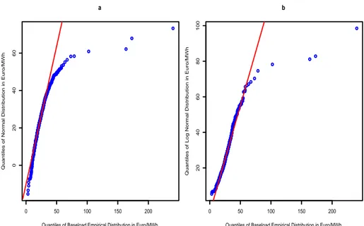
usually rather seem to follow a lognormal than a normal distribution. Therefore, most authors, e.g. Escribano et al. (2002), Burger et al.(2004), and de Jong and Huisman (2003), prefer working with the logarithm of power prices instead of the original price series. Here, we follow their approach. Furthermore, Figure 2.2.2 shows the quantile-quantile plots of baseload against a normal distribution and a lognormal distribution, respectively. The superimposed lines in subfigures 2.2.2a and 2.2.2b pass through the first and third quartile and help to assess the deviation from the straight line.

According to e.g. Escribano et al. (2002) and de Jong and Huisman (2003) the logarithm of power prices log(P t ) will be assumed to consist of two parts, a deter- ministic part denoted by f t and a stochastic part X t ,

log(P t ) = f t + X t . (2.2.3)

Figure 2.2.3 shows the weekly seasonality. In order to take into account the weekly seasonality, weekend dummy variables for Saturdays and Sundays as well as a dummy variable for holidays are included. Moreover, since the range of the data covers more than four years, we include a deterministic linear trend and a sinu- soidal term to consider yearly seasonality.

The deterministic part of the logarithm of the power price f t is specified as, f t = β 1 · dummy sat + β 2 · dummy sun + β 3 · dummy hol + β 4 · t

+γ 1 · sin µ

(γ 2 + t) · 2π 365

¶

. (2.2.4)

More precisely, dummy sat is the dummy variable for Saturdays, whereas dummy sun

is the dummy variable for Sundays. The dummy variable for holidays is denoted

dummy hol . Finally, t is linear trend measured in days. The deterministic compo-

nent f t is estimated jointly with the parameters of the stochastic model of interest.

a

Month and Year

Euro/MWh

6/2000 1/2001 1/2002 1/2003 1/2004 7/2004

0 50 100 150 200 240

Baseload

b

Month and Year

log(Euro/MWh)

6/2000 1/2001 1/2002 1/2003 1/2004 7/2004

0 1 2 3 4 5

log(Baseload)

Mon Tue Wed Thu Fri Sat Sun

0 1 2 3 4 5

Mon Tue Wed Thu Fri Sat Sun

0 1 2 3 4 5 6

c

log(Euro/MWh)

d

Month and Year

MWh

6/2000 1/2001 1/2002 1/2003 1/2004 7/2004

0 75000 150000 210000

Volume

Figure 2.2.1: Plots for baseload spot prices, the logarithm of baseload spot prices,

log(baseload), and the traded volume at the EEX.

0 50 100 150 200

0 20 40 60

a

Quantiles of Baseload Empirical Distribution in Euro/MWh

Quantiles of Normal Distribution in Euro/MWh

0 50 100 150 200

20 40 60 80 100

b

Quantiles of Baseload Empirical Distribution in Euro/MWh

Quantiles of Log Normal Distribution in Euro/MWh

Figure 2.2.2: Quantile-quantile plots for baseload spot prices at the EEX.

hour

Price in EUR/MWh

0 24 48 72 96 120 144 168

0 10 20 30 40 50 60

Mon Tue Wed Thu Fri Sat Sun

Weekly seasonality

Figure 2.2.3: Weekly seasonality of baseload spot prices at the EEX.

2.3 Stochastic Models for Power Prices

In this section, we discuss some of the models for the stochastic part of electricity spot prices with a special focus on Markov regime-switching models.

2.3.1 AR(1) Process with Drift

We include the AR(1) process as a linear benchmark model. Although this process captures mean reversion, which is a main stylized fact of electricity prices, it cannot take into account spikes. The mean to which the process reverts is µ _M . M refers to mean reversion in the remainder of the thesis.

X _t = ρ · µ _M + (1 − ρ) · X _t−1 + ² _M,t , ² _M,t ∼ N (0, σ ² _M ). (2.3.1)

2.3.2 The Jump Model

Stochastic jump diffusion models with mean reversion are a very popular approach for the modelling of electricity prices. The mean reversion component is used to force prices to revert to a normal level after a spike has occurred. We find two procedures to cope with spikes in jump models.

In the first approach, spikes are extracted if they exceed an arbitrarily set thresh- old. The extracted prices are then replaced by the arithmetic average of the neighboring prices, for example. This kind of preprocessing procedure is advo- cated by Cuaresma et al. (2004) and Weron (2006). The extracted spikes are then exploited to specify a spike distribution. The intensity of the jump process is determined by the frequency of detected spikes in the data. The data, from which spikes have been extracted, is used to estimate the remaining parameters.

Secondly, we can simply specify a model which allows to simultaneously estimate all model parameters by means of maximum likelihood. The second procedure is applied by Escribano et al. (2002), Huisman and Mahieu (2003) as well as by Knittel and Roberts (2005). Here, we follow the approach presented in Huisman and Mahieu (2003). Hence, we model mean reversion similar to equation (2.3.1).

The jumps J t are assumed to be each the sum of independently and identically dis- tributed normals Z i,t . In addition, we assume Z i,t ∼ N (µ S , σ _S ² ) with i = 1, . . . , n t , mean µ S and variance σ _S ² . The arrival process of the compound jumps is modelled by a Poisson distribution with intensity λ,

X t = ρ · µ M + (1 − ρ) · X t−1 + ² M,t +

n t

X

i=1

Z i,t , ² M,t ∼ N (0, σ ² _M ) . (2.3.2) Let LL denote the logarithmic likelihood,

LL =

−T · λ − T

2 ln(2π) + (2.3.3)

X T

t=1

ln



 X ∞

j=0

λ ^j j!

p 1

σ _M ² + jσ _S ² exp µ

− (X t − ρ · µ M + (1 − ρ) · X t−1 − jµ S ) ² 2(σ ² _M + jσ ² _S )

¶ 

 .

Following Huisman and Mahieu (2003), we compute the sum P ^∞

j=0

. . . up to j = 10.

Estimation is carried out by maximizing LL with respect to the model parameters.

We gauge models by means of information criteria. The information criteria of Akaike (AC) and Schwartz (SC) are computed as follows throughout the thesis,

AC = −2 · LL + 2k

T SC = −2 · LL + k log(T )

T .

Moreover, k denotes the number of estimated parameters and T the number of observations. The jump model provides a notably better fit than the AR(1) model Table 2.3.1: Results on the AR(1) Model, equation(2.3.1), and the Jump Model, equation (2.3.2).

AR(1) Jump Model

log(baseload) log(peakload) log(baseload) log(peakload) β 1 −0.285

(0.014)

−0.360 (0.021)

−0.270 (0.009)

−0.337 (0.012)

β 2 −0.579 (0.014)

−0.682 (0.019)

−0.556 (0.010)

−0.645 (0.012)

β 3 −0.597 (0.018)

−0.812 (0.021)

−0.507 (0.017)

−0.638 (0.020)

β 4 0.0003

(4.5·10 ⁻⁷ )

0.0003 (4.5·10 ⁻⁷ )

0.0003 (3·10 ⁻⁷ )

0.0003 (3·10 ⁻⁷ )

γ 1 0.099

(0.020

0.098 (0.022)

−0.124 (0.016)

0.112 (0.015)

γ 2 −90.18 (15.341)

−67.57 (14.304)

−87.141 (8.680)

−79.940 (8.680)

µ M 3.041

(0.039)

3.259 (0.038)

3.021 (0.026)

3.228 (0.023)

ρ _(0.011) ^0.337 _(0.010) ^0.428 _(0.013) ^0.327 _(0.014) ^0.414

σ M 0.194

(0.001)

0.237 (0.002)

0.141 (0.003)

0.156 (0.004)

λ - - _(0.013) ^0.066 _(0.016) ^0.091

µ S - - _(0.058) ^{0.036 ∗} _(0.050) ^{0.079 ∗}

σ S - - _(0.040) ^0.506 _(0.036) ^0.556

LL 333.83 32.20 543.68 317.89

AC -0.4322 -0.0309 -0.7075 -0.4070

SC -0.4004 0.0010 -0.6651 -0.3646

Note that ^∗ means not significant at the 5 % level.

for the logarithm of baseload and peakload, respectively. Moreover, all param-

eter estimates in table 2.3.1 are highly significant except for the estimate of µ s ,

which is not significant at the 5 % level. In Figure 2.2.1c, we see that upward and

downward deviations are inherent in the logarithm of daily spot prices. This may

explain why the estimate of µ s is not significant at the 5 % level. All results are

presented in table 2.3.1.

Jump models are a very popular approach with derivative valuation based on spot prices. However, jump models have certain shortcomings. As pointed out by Huis- man and Mahieu (2003), it is not easy to disentangle jumps from the estimation of the parameter ρ which governs the degree of mean reversion. Secondly, these models are not suitable for forecasting. Albeit, a successful attempt to predict spot prices with jump models has been undertaken by Cuaresma et al. (2004), their implemented forecasting procedure is rather heuristic and should be treated with caution.

2.3.3 A Markov Regime-Switching Model for Spot Prices:

Ethier and Mount(1998)

Besides the jump model, Markov regime-switching approaches are widely consid- ered as tailor-made to model spot prices. These models are based on the Markov regime-switching model of Hamilton (1989) which has originally been put forward to model the business cycle of the economy in the USA. The basic idea of the model is that the economy switches between one or more different regimes. For example, we can assume a boom regime and a recession regime. Furthermore in the basic approach, we assume that the regime-switching mechanism is exogenous and the prevailing regime is latent. By this, we presume that we do not know exactly which regime prevails at a certain point in time. However, we can at least express a certain regime probability. Moreover, we presume to know the probabil- ity of transition from one regime to another.

Indeed, it seems very convincing to classify occasional spikes and normal prices in different regimes. To the best of our knowledge, the first attempt to model spot prices with Markov regime-switching models has been undertaken by Ethier and Mount (1998). Analogously to the original model, Ethier and Mount specify a two- regime model. One regime to model normal prices and the second to capture spikes. Contrary to the basic model proposed by Hamilton (1989), they assume heteroscedasticity. By this, each regime is assigned its own variance. The prevail- ing regime at time t is denoted S t . In the remainder of the thesis, we set S t = M when power prices are in the normal regime and S t = S else. Additionally, we refer to the normal regime as the stable regime in the remainder of the thesis. We present the model of Ethier and Mount (1998) in equations (2.3.4 - 2.3.6)

X M,t = µ M + (1 − ρ) · ¡

X _{{S t−1 =i},t−1} − µ _{{S t−1 =i}} ¢

+ ² M,t , (2.3.4) X S,t = µ S + (1 − ρ) · ¡

X {S t−1 =i},t−1 − µ {S t−1 =i}

¢ + ² S,t , (2.3.5)

with i ∈ {M, S}, ² M,t ∼ N (0, σ ² _M ), ² S,t ∼ N (0, σ ² _S ) .Transition between the regimes is governed by the transition matrix Π,

Π =

à q 1 − p 1 − q p

!

, (2.3.6)

where, q denotes the probability to stay in the stable regime, and p denotes the probability to stay in the spike regime. In addition, X M,t denotes the value of X t

provided that S t = M and X S,t the same with S t = S.

2.3.4 Two-Regime Model with Independent Spikes : De Jong and Huisman (2003)

The second attempt to model spot prices with Markov regime-switching models has been made by Huisman and Mahieu (2003). These authors put forward a three- regime model. They propose two spike regimes where one spike regime is designed to pull the price process back to the stable regime after a spike has occured. This three- regime model is conceived to better disentangle spikes from the stable regime than a jump model does. A shortcoming of this model is that it does not allow for consecutive spikes. Hence, the price process cannot stay in the spike regime.

However, consecutive spikes are convenient with the fact that unforced outages can have a longer impact on spot prices than one day. To overcome this disadvantage and to allow consecutive spikes, De Jong and Huisman (2003) advocate a two- regime model with independent spikes. The authors assume one spike regime and one stable regime. The stable regime is modelled as follows,

X M,t = X M,t−1 + ρ · (µ M − X M,t−1 ) + ² M,t , ² M,t ∼ N (0, σ _M ² ) , (2.3.7) whereas for the spike regime, the authors assume,

X S,t = µ S + ² S,t , ² S,t ∼ N (0, σ _S ² ) . (2.3.8) Transition between the states is governed by the same transition matrix Π as in the Model of Ethier and Mount (1998), which is given in equation (2.3.6).

Up to now, it is not clear why spikes in this model are called independent. This is the peculiarity of the model. The authors assume that the stable regime latently evolves untouched through time, while a spike occurs. Hence, they assume two stochastic processes which independently evolve next to each other through time.

However, at each point in time, we can only observe the realization of one of the two processes. For example, we may observe a spike at t and a normal price at t − 1. To obtain an unbiased estimation of the stable regime process, we have to include the latent value of the stable regime at t, which we did not observe. To solve the problem, De Jong and Huisman (2003) suggest to go back to t − 1, where we assume the price to originate from the stable regime and to approximate the latent value of the stable regime at t by its forecast based on the normal price at t − 1. It sounds easy, but, as a result, a very complex logarithmic likelihood has to be constructed.

The aim of De Jong and Huisman (2003) is to disentangle spikes from the stable regime as well as possible, without having to include an additional regime to pull prices back to the stable regime, as suggested by Huisman and Mahieu (2003).

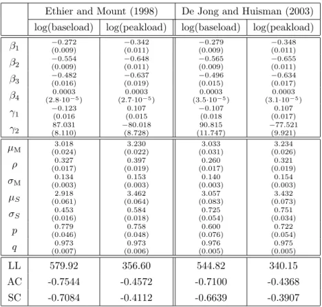
In fact, if we compare the results of the two regime model of Ethier and Mount

(1998)in table 2.3.2 with the results of De Jong and Huisman (2003), we observe

that the estimate of ρ is smaller in the two regime model of De Jong and Huisman

(2003) than in the model of Ethier and Mount (1998) for both considered time

series. Moreover, the estimate of p is also smaller, whereas the estimate of q is

larger in the De Jong and Huisman (2003) model than in the model of Ethier

and Mount (1998). All these results indicate that the approach of De Jong and

Huisman (2003) is capable of better disentangling spikes from the stable regime

than the model put forward by Ethier and Mount (1998). This is especially true for the logarithm of baseload. By contrast, for the logarithm of peakload the difference between the model results is smaller.

Table 2.3.2: Results on the Two-Regime Switching Models, see equations (2.3.4- 2.3.8).

Ethier and Mount (1998) De Jong and Huisman (2003) log(baseload) log(peakload) log(baseload) log(peakload) β 1 −0.272

(0.009)

−0.342 (0.011)

−0.279 (0.009)

−0.348 (0.011)

β 2 −0.554

(0.009) −0.648

(0.011) −0.565

(0.009) −0.655

(0.011)

β 3 −0.482

(0.016) −0.637

(0.019) −0.496

(0.015) −0.634

(0.017)

β 4 0.0003

(2.8·10 ⁻⁵ ) 0.0003

(2.7·10 ⁻⁵ ) 0.0003

(3.5·10 ⁻⁵ ) 0.0003 (3.1·10 ⁻⁵ )

γ 1 −0.123 (0.016

0.107 (0.015

−0.107 (0.018

0.107 (0.017)

γ 2 87.031

(8.110)

−80.018 (8.728)

90.815 (11.747)

−77.521 (9.921)

µ M 3.018

(0.024) 3.230

(0.022) 3.033

(0.031) 3.234

(0.026)

ρ _(0.017) ^0.327 _(0.019) ^0.397 _(0.017) ^0.260 _(0.019) ^0.321

σ M 0.134

(0.003)

0.153 (0.003)

0.140 (0.003)

0.154 (0.003)

µ S 2.918

(0.061)

3.462 (0.064)

3.057 (0.083)

3.432 (0.073)

σ S 0.453

(0.016)

0.584 (0.018)

0.725 (0.054)

0.751 (0.034)

p _(0.046) ^0.779 _(0.048) ^0.758 _(0.076) ^0.600 _(0.054) ^0.722 q _(0.007) ^0.973 _(0.006) ^0.973 _(0.005) ^0.976 _(0.005) ^0.975

LL 579.92 356.60 544.82 340.15

AC -0.7544 -0.4572 -0.7100 -0.4368

SC -0.7084 -0.4112 -0.6639 -0.3907

2.3.5 Estimation of Markov Regime-Switching Models

Here, we explain how the logarithmic likelihoods for the models of interest can be constructed. Let LL = P _T

t=1 ln f (X t |F t−1 ) be the logarithmic likelihood. Here, F t−1 denotes the information set at t − 1. The conditional density is expressed as follows:

f (X t |F t−1 ) = f (X t , S t = M |F t−1 ) + f (X t , S t = S|F t−1 ) (2.3.9)

= f (X t |S t = M, F t−1 ) · f (S t = M |F t−1 ) +

f (X t |S t = S, F t−1 ) · f (S t = S|F t−1 )

Moreover, the density f (S t = i|F t−1 ), i ∈ {M, S}, has to be determined. It holds (j ∈ {M, S} ),

f (S t = j|F t−1 ) = f (S t = j, S t−1 = M |F t−1 ) + f (S t = j, S t−1 = S|F t−1 )

= f (S t = j|S t−1 = M ) · f (S t−1 = M |F t−1 )

+ f (S t = j|S t−1 = S) · f (S t−1 = S|F t−1 ). (2.3.10)

The terms f (S _t = j|S _t−1 = i) are the one-step transition probabilities.

Conditional probabilities of type f (S t−1 = j|F t−1 ) are recursively calculated.

Due to F t−1 = {F t−2 , X t−1 } it holds

f(S t−1 = j|F t−1 ) = f (S t−1 = j|F t−2 , X t−1 ) = f (S t−1 = j, X t−1 |F t−2 )

f (X t−1 |F t−2 ) (2.3.11)

= f (X t−1 |S t−1 = j, F t−2 ) · f (S t−1 = j|F t−2 ) P

i={M,S} f (X t−1 |S t−1 = i, F t−2 ) · f (S t−1 = i|F t−2 ) .

According to Hamilton (1989), we can further decompose the densities in equation (2.3.9), f (X t |S t = M, F t−1 ), f(X t |S t = S, F t−1 ), and compute f (X t |F t−1 ) as given in equation (2.3.12),

f(X t |F t−1 ) =

f (X _t |S _t = M, S _t−1 = M |F _t−1 ) · f (S _t = M, S _t−1 = M |F _t−1 ) (2.3.12) + f (X t |S t = M, S t−1 = S|F t−1 ) · f (S t = M, S t−1 = S|F t−1 )

+ f (X t |S t = S, S t−1 = M |F t−1 ) · f (S t = S, S t−1 = M |F t−1 ) + f (X t |S t = S, S t−1 = S |F t−1 ) · f(S t = S, S t−1 = S|F t−1 ) .

Note that in this case spikes enter the stable regime due to f (X t |S t = M, S t−1 = S|F t−1 ). De Jong and Huisman (2003) want to avoid this effect. Therefore, they do not decompose f (X t |S t = M, F t−1 ) as in equation (2.3.12) but replace the part of the conditional density that represents the stable regime f (X t |S t = M, F t−1 ) by an approximation,

f(X t |S t = M, F t−1 ) ≈ X K

i=1

P rob[S t−i = M ∧S t−j 6= M for j < i]·f (X t |S t = M, F t−i ) The key problem in calibrating this conditional density is the determination of the value of X M,t−i , where i = 1, . . . K, because the last spot price originating from the stable regime is not known. K denotes how far we maximally go back to find the last spot price originating from the stable regime.

f(X t |S t = M, F t−i ) ≈ 1 V ar[X M,t |F t−i ] · √

2π · exp µ

− (X M,t − E[X M,t |F t−i ]) ² 2 · V ar[X M,t |F t−i ]

¶

with

E[X M,t |F t−i ] = ρ · µ M + (1 − ρ) · E[X M,t−1 |F t−i ] , (2.3.13)

V ar[X M,t |F t−i ] = σ _M ² + (1 − ρ) ² · V ar[X M,t−1 |F t−i ] . (2.3.14)

Applying these equations for the conditional expectations and variances yields E[X M,t |F t−i ] = (1 − ρ) ⁱ · X M,t−i + µ M · (1 − (1 − ρ) ⁱ ) , (2.3.15)

V ar[X M,t |F t−i ] = σ _M ² · (1 − ρ) ^2·i − 1

(1 − ρ) ² − 1 . (2.3.16) The expression P rob[S t−i = M ∧ S t−j 6= M for j < i] is the probability of the logarithm of the spot price X t−i to be the last logarithm of the spot price before X t

originating from the stable regime. X t−j with j < i, whereas, are supposed to be spikes. The remaining problem is to determine the right K. De Jong and Huisman (2003) propose K = 5. In our calculations, K = 5 appears to be sufficient, too.

2.3.6 Regime-Switching Models with Day-Dependent Spikes:

Kosater and Mosler (2006)

The models proposed by Ethier and Mount (1998) and De Jong and Huisman (2003) assume that deviations from the stable regime are independent of the type of the day. However, it seems more sensible to distinguish between working days on one hand and weekends and holidays on the other. Very low demand is typical of weekends and holidays. Therefore, upward directed spikes are rather not to be expected, whereas we can detect downward directed deviations from the stable regime in our German data. In order to take into account different types of days, Kosater and Mosler (2006) put forward to distinguish between high spikes and low spikes.

Practically, they decompose spikes by introducing an indicator function 1 H which takes the value zero on holidays, weekend days, and two days before and after a holiday. All remaining days are candidates for high spikes only, therefore for these days the indicator function takes value 1. The decomposition fits well to observed German data. However, weekends, at least Sundays, and holidays are days of low demand not only in Germany. In fact, De Jong (2006) finds that the decomposition put forward by Kosater and Mosler (2006) works well for a number of international markets, too.

1 H =

 



0 holiday, weekend, two days before and after a holiday ,

1 else . (2.3.17)

Since for both two-regime models, the authors only modify the spike regime, the stable regime is left unchanged with respect to the original models. Moreover, transition between the regimes is assumed to be governed by the transition matrix Π. The authors extend the spike regime in De Jong and Huisman (2003) as follows, X S,t = 1 H · (µ S,H + ² S,H,t ) + (1 − 1 H )· (µ S,L + ² S,L,t ) spike regime . (2.3.18) Additionally, they assume that the disturbances in the high spike regime denoted

² S,H,t and the low spike regime denoted ² S,L,t are both normally distributed with possibly different variances, ² S,H,t ∼ N (0, σ _S,H ² ) and ² S,L,t ∼ N (0, σ ² _S,L ).

Kosater and Mosler (2006) analogously extend the model of Ethier and Mount

(1998),

X S,t = µ S + (1 − ρ) · ¡

X _{{S t−1 =i},t−1} − µ _{{S t−1 =i}} ¢

+ ² S,t , (2.3.19) µ S = 1 H · (µ S,H ) + (1 − 1 H ) · (µ S,L ) , (2.3.20)

² S,t = 1 H · (² S,H,t ) + (1 − 1 H ) · (² S,L,t ) , (2.3.21)

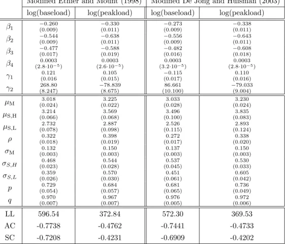
where j, i ∈ {M, S}, ² M,t ∼ N (0, σ ² ), ² S,H,t ∼ N (0, σ _S,H ² ), ² S,L,t ∼ N (0, σ _S,L ² ) . The results for the two- regime models with a day-dependent spike regime are collected in table 2.3.3. More precisely, table 2.3.3 shows that the modified mod- els put forward by Kosater and Mosler (2006) outperform the original versions of Ethier and Mount (1998) and De Jong and Huisman (2003) in terms of fit.

This result is also clearly confirmed by both information criteria. All parameter estimates are significant. Hence, the introduction of day-dependent spikes is a worthwhile extension.

In addition to the estimation results presented in tables 2.3.2-2.3.3, Figure 2.3.1 presents the smoothed probabilities for the considered Markov regime-switching approaches. Furthermore, Figure 2.3.2 shows quantile-quantile plots for the log- arithm of baseload series from which the deterministic effects have been removed against simulated series from the discussed Markov regime-switching approaches.

In more detail, the smoothed probabilities are computed as follows. Let ξ t|t be the vector of filtered regime probabilities at time t given the information at time t. We calculate the smoothed regime probabilities at time t given the information at time T , ξ t|T , according to Kim (1994):

ξ _t|T = ξ _t|t ¯ {Π ⁰ £

ξ _t+1|T ÷ ξ _t+1|t ¤

} . (2.3.22)

Note that ¯ is the element by element product, whereas ξ _t+1|T ÷ ξ _t+1|t symbolizes element by element division.

To summarize the results of the in-sample study, the models without independent spikes provide slightly higher spike probabilities than the models with independent spikes and outperform their independent counterparts in terms of fit, in particular for the logarithm of baseload.

Finally, the quantile-quantile plots in Figure 2.3.2 show that the simulated series

generated from the models put forward by Kosater and Mosler (2006) are notably

closer to the empirical series than simulated series from the original models of

Ethier and Mount (1998) as well as De Jong and Huisman (2003). For the loga-

rithm of baseload, the model without independent spikes of Kosater and Mosler

(2006) performs best.

Table 2.3.3: Results on Two- Regime Models with Day-Dependent Spikes, see equations (2.3.17-2.3.21).

Modified Ethier and Mount (1998) Modified De Jong and Huisman (2003) log(baseload) log(peakload) log(baseload) log(peakload) β 1 −0.260

(0.009)

−0.330 (0.011)

−0.273 (0.009)

−0.338 (0.011)

β 2 −0.544 (0.009)

−0.638 (0.011)

−0.556 (0.009)

−0.643 (0.011)

β 3 −0.477 (0.017)

−0.588 (0.019)

−0.482 (0.016)

−0.608 (0.018)

β 4 0.0003

(2.8·10 ⁻⁵ )

0.0003 (2.6·10 ⁻⁵ )

0.0003 (3.2·10 ⁻⁵ )

0.0003 (2.8·10 ⁻⁵ )

γ 1 0.121

(0.016

0.105 (0.015)

−0.115 (0.017)

0.110 (0.016)

γ 2 268.80

(8.247)

−78.839 (8.675)

86.661 (10.100)

−79.033 (9.004)

µ M 3.018

(0.024)

3.225 (0.022)

3.033 (0.028)

3.230 (0.024)

µ S,H 3.214

(0.066)

3.569 (0.068)

3.496 (0.100)

3.835 (0.083)

µ S,L 2.732

(0.078)

2.887 (0.098)

2.526 (0.115)

2.893 (0.124)

ρ _(0.018) ^0.322 _(0.019) ^0.398 _(0.017) ^0.272 _(0.020) ^0.338

σ M 0.132

(0.003)

0.150 (0.003)

0.137 (0.003)

0.150 (0.003)

σ S,H 0.468

(0.023)

0.544 (0.028)

0.537 (0.045)

0.530 (0.033)

σ S,L 0.359

(0.026) 0.570

(0.030) 0.451

(0.061) 0.605

(0.042)

p _(0.054) ^0.729 _(0.057) ^0.684 _(0.065) ^0.681 _(0.049) ^0.736 q _(0.007) ^0.970 _(0.007) ^0.967 _(0.005) ^0.976 _(0.006) ^0.972

LL 596.54 372.84 572.30 369.53

AC -0.7738 -0.4762 -0.7441 -0.4733

SC -0.7208 -0.4231 -0.6909 -0.4202

a

Month and Year

log(Euro/MWh)

6/2000 1/2001 1/2002 1/2003 1/2004

0 1 2 3 5 7 9

log(baseload) smoothed probability

b

Month and Year

log(Euro/MWh)

6/2000 1/2001 1/2002 1/2003 1/2004

0 1 2 3 5 7 9

log(baseload) smoothed probability

c

Month and Year

log(Euro/MWh)

6/2000 1/2001 1/2002 1/2003 1/2004

0 1 2 3 5 7 9

log(baseload) smoothed probability

d

Month and Year

log(Euro/MWh)

6/2000 1/2001 1/2002 1/2003 1/2004

0 1 2 3 5 7 9

log(baseload) smoothed probability

Figure 2.3.1: Plots showing smoothed spike regime probabilities for the following

models: (a) Ethier and Mount (1998), (b) De Jong and Huisman (2003), (c)

Kosater and Mosler (2006)(without independent spikes), (d) Kosater and Mosler

(2006) (with independent spikes).

2 3 4 5

123456

a

Quantiles of the Empirical Distribution

Quantiles of the Simulated Distribution

2 3 4 5

123456

b

Quantiles of the Empirical Distribution

Quantiles of the Simulated Distribution

2 3 4 5

123456

c

Quantiles of the Empirical Distribution

Quantiles of the Simulated Distribution

2 3 4 5

123456

d

Quantiles of the Empirical Distribution

Quantiles of the Simulated Distribution

Figure 2.3.2: Quantile-quantile plots for log(baseload) from which the determinis-

tic effects have been removed against the estimated models: (a) Ethier and Mount

(1998), (b) De Jong and Huisman (2003), (c) Kosater and Mosler (2006)(with-

out independent spikes), (d) Kosater and Mosler (2006) (with independent spikes),

(Note: To guarantee comparability, two elements in each simulated series through-

out the four plots are set equal to 1 and 6, respectively).