Loss Given Default of Leasing Contracts
Inauguraldissertation zur
Erlangung des Doktorgrades der
Wirtschafts- und Sozialwissenschaftlichen Fakultät der
Universität zu Köln 2016
vorgelegt von
Dipl.-Wirt.-Math. Patrick Michel Miller aus
Leverkusen
Vorsitz: Univ.-Prof. Dr. Heinrich R. Schradin, Universität zu Köln
Tag der Promotion: 11. Januar 2017
The completion of this thesis would not have been possible without being sup- ported by many people, whom I would like to thank.
Most of all, I would like to express my gratitude to my advisor Professor Dr.
Thomas Hartmann-Wendels for his support, motivation and incredibly helpful suggestions during my research. Moreover, I would also like to thank him for the opportunity to present my studies at several meetings and, in particular, international conferences. Another word of thanks is addressed to Professor Dr.
Dieter Hess for serving as co-referee and to Professor Dr. Heinrich R. Schradin for chairing the dissertation committee.
My sincere gratitude also goes to Dr. Eugen Töws for the great collaboration.
We had countless extensive and productive discussions on several topics that re- sulted in two co-authored projects. I really appreciate the joint research with him.
I would also like to thank my former colleagues at the University of Cologne. I would like to mention Patrick Wohl, Dr. Tobias Schlüter, Benjamin Döring, David Fritz, Elke Brand, Dr. Claudia Wendels and, in particular, Dr. Wolfgang Spörk for their support and their valuable suggestions and advices on various topics.
Further thanks go to all of my friends for their motivation. In particular, I would like to thank Benjamin Rombelsheim for several discussions and for his support.
Finally, I would like to express my deepest gratitude to my parents Horst and Bettina Miller for the continuous encouragement and tremendous support that made the completion of this thesis possible. I would also like to thank my girlfriend Monika Wieczorek for her patience, motivation and support. Moreover, my thanks go to the rest of my family and in particular I would like to say thank you to my grandfather Franz Josef Bock, who passed away way too early, for his unbounded confidence in every single life situation.
Cologne, January 2017 Patrick Michel Miller
default for leasing: Parametric and nonparametric estimations. Journal of Banking & Finance 40, 364–375.
Patrick Miller, 2015. Does the Economic Situation Affect the Loss Given Default of Leases?. Working paper.
Patrick Miller and Eugen Töws, 2016. Loss Given Default-Adjusted Workout
Processes for Leases. Working paper.
List of Abbreviations xi
List of Figures xiii
List of Tables xiv
1 Introduction 1
1.1 Estimating the loss given default: an initial literature review . . . 5
1.2 Contents and structure of the thesis . . . . 12
2 Loss given default for leasing: Parametric and nonparametric estimations 18 2.1 Introduction . . . . 18
2.2 Literature review . . . . 20
2.3 Data set . . . . 23
2.4 Methods . . . . 28
2.4.1 Finite mixture models and classification . . . . 30
2.4.2 Regression and model trees . . . . 31
2.4.3 Out-of-sample testing . . . . 34
2.5 Results . . . . 35
2.5.1 In-sample results . . . . 37
2.5.2 Out-of-sample results . . . . 39
2.5.3 Validation and interpretation . . . . 45
2.6 Conclusion . . . . 50
3 Does the Economic Situation Affect the Loss Given Default of Leases? 52 3.1 Introduction . . . . 52
3.2 Data . . . . 58
3.2.1 Fluctuations of the LGD . . . . 61
3.2.2 Workout Characteristics . . . . 63
3.2.3 Explanatory Idiosyncratic Factors . . . . 65
3.2.4 Explanatory Macroeconomic Factors . . . . 69
3.3 Methods . . . . 73
3.3.1 Regression Splines . . . . 75
3.3.2 Performance Measurements . . . . 76
3.3.3 Out-of-time Testing . . . . 78
3.4 In-sample Analysis . . . . 79
3.4.1 Analysis of the Idiosyncratic Factors . . . . 83
3.4.2 Analysis of the Macroeconomic Factors . . . . 87
3.5 Out-of-time Analysis . . . . 92
3.5.1 Results at Execution of the Contract . . . . 92
3.5.2 Results at Default of the Contract . . . . 95
3.5.3 Interpretation and Implications . . . . 99
3.6 Conclusion . . . 103
3.7 Appendix . . . 106
4 Loss Given Default-Adjusted Workout Processes for Leases 107 4.1 Introduction . . . 107
4.2 Related literature . . . 110
4.3 Dataset . . . 113
4.4 Methods . . . 121
4.4.1 Direct estimation . . . 122
4.4.2 Loss given default decomposition . . . 124
4.4.3 Loss given default classification . . . 125
4.4.4 Validation techniques . . . 127
4.4.5 Performance measurements . . . 130
4.5 Results . . . 132
4.5.1 In-sample validation . . . 133
4.5.2 Out-of-sample validation . . . 134
4.5.3 Out-of-time validation . . . 136
4.5.4 Further estimation and classification . . . 138
4.5.5 Interpretation . . . 141
4.6 Conclusion . . . 146
5 Summary and conclusions 148
Bibliography 152
AIC Akaike information criterion ALGD Asset-related loss given default ARR Asset-related recovery rate
BDL Federal Association of German Leasing Companies BIC Bayesian information criterion
CRR Capital Requirement Regulation EAD Exposure at default
FMM Finite mixture model
ICT Information and communication technology IRBA Internal Ratings Based Approach
k NN k -nearest neighbor LGD Loss given default MAE Mean absolute error
MLGD Miscellaneous loss given default MRR Miscellaneous recovery rate MSE Mean squared error
MURD Moody’s Ultimate Recovery Database
NAREC Normalized area under the regression error characteristic curve OLS Ordinary least squares
PD Probability of default
REC Regression error characteristic
REC Area Area under the regression error characteristic curve
RF Random forest
RMSE Root mean squared error
RR Recovery rate
RT Regression tree
TIC Theil inequality coefficient
2.1 Density of realized loss given default by company. . . . 26 2.2 Density of realized loss given default by company for the three
major asset types: vehicles, machinery, and information and com- munications technology. . . . 28 2.3 Densities of realized loss given default, loss given default estimated
by ordinary least squares regression without variable selection, and loss given default estimated by finite mixture combined with 3- nearest neighbors for company B. . . . 46 2.4 Scatter plot of realized and in-sample and out-of-sample estimated
loss given default. . . . 47 3.1 Density of the realized loss given default for company A and B. . 60 3.2 Evolution of the macroeconomic factors in the period from 01/1998
to 12/2009. . . . 71 3.3 Influence of the economic situation. . . . 88 3.4 Regression error characteristic curves of the out-of-time loss given
default estimations at default of the contract for company A by forecast period. . . . 97 4.1 Densities of the two classes of the loss given default, after separating
the contracts according to their relationship of loss given default to asset-related loss given default. . . 117 4.2 Densities of the shares of loss given default, asset-related loss given
default and miscellaneous loss given default. . . 118
4.3 Procedure of the developed models. . . 123
4.4 Procedure of the used validation techniques. . . 128
4.5 Visual comparison of the realized and estimated loss given default. 142
2.1 Numbers of contracts and lessees in the data sets of companies A–C in descending order of the number of contracts. . . . 23 2.2 Loss given default density information for companies A–C. . . . . 25 2.3 Loss given default density information by asset type for companies
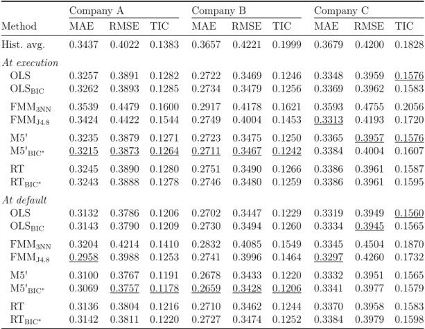
A–C. . . . 27 2.4 In-sample estimation errors at the execution and default of con-
tracts by company. . . . 37 2.5 Out-of-sample estimation errors at the execution and default of
contracts by company. . . . 39 2.6 Out-of-sample estimation errors at the execution and default of
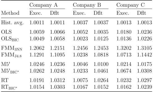
contracts by sample size. . . . 43 2.7 Janus quotient for in-sample and out-of-sample estimations of loss
given default for each method and company at execution and de- fault of the contracts. . . . 45 2.8 In-sample classification errors for the 3-nearest neighbors and J4.8
methods at execution and default of the contracts. . . . 48 3.1 Number of contracts and lessees in the datasets of the companies
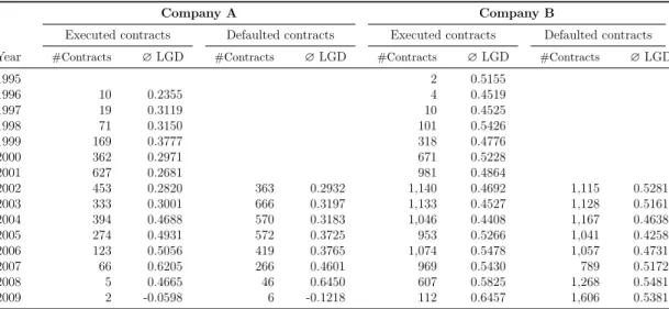
A and B. . . . 58 3.2 Number of executed respectively defaulted contracts and related
average loss given default, by year and company. . . . 61 3.3 Average share and standard deviation of the inflows from disposing
the leased asset respectively through customer payments in relation to the total inflows received during the workout, by company and year of default. . . . 63 3.4 Number of contracts with completed workout at the end of year t
that are used for model fitting. . . . 78 3.5 In-sample performance measurements at execution and default of
the contracts by company. . . . 80
3.6 In-sample coefficient estimates at execution of the contracts. . . . 81
3.7 In-sample coefficient estimates at default of the contracts. . . . 82
3.8 Out-of-time performance measurements at execution of the con- tract by company and forecast period. . . . 93 3.9 Out-of-time performance measurements at default of the contract
by company and forecast period. . . . 96 4.1 Numbers of contracts and lessees as well as loss given default and
exposure at default key figures of the dataset. . . 113 4.2 Distribution parameters of the loss given default. . . 116 4.3 Distribution parameters of the loss given default for each default
year. . . 120 4.4 Year of default and frequency of contracts. . . 130 4.5 Consistent set of variables used for regression and classification. . 133 4.6 In-sample loss given default estimation results. . . 133 4.7 Out-of-sample loss given default estimation results. . . 134 4.8 Out-of-time loss given default estimation results. . . 136 4.9 Asset-related loss given default and miscellaneous loss given default
estimation results. . . 138 4.10 Classification results. . . 139 4.11 Classification results, considering exclusively classification proba-
bilities below 25% or above 75%. . . 141
4.12 Performance improvements in loss given default estimation literature.144
Risk management is of crucial importance for financial institutions. Identifying and quantifying the risk related to financial instruments is essential to make eco- nomically and strategically reasonable decisions. In particular, the knowledge of potential losses of financial assets is substantial for properly allocating regulatory and economic capital.
One of the major concerns of financial institutions’ risk management is credit risk. Together with the probability of default (PD) and the exposure at default (EAD), the credit risk of a financial asset is particularly determined by the loss given default (LGD) respectively its counterpart, the recovery rate. The LGD is defined as the percentage of the EAD the financial institution loses if a debtor defaults.
According to Article 107 (1) of the Capital Requirement Regulation (CRR), financial institutes shall apply either the Standardised Approach or the Internal Ratings Based Approach (IRBA) to calculate their regulatory capital requirements for credit risk. To implement the advanced IRBA requires financial institutes to develop internal models for estimating PD, EAD, and LGD. One of the main objectives of the IRBA, which was introduced by the banking regulation within Basel II, the predecessor of the CRR, is to achieve risk-adjusted capital require- ments (see Basel Committee on Banking Supervision (2003)). However, accurate estimates of PD, EAD, and LGD are also beneficial for pricing financial instru- ments and may lead to competitive advantages in general, as Gürtler and Hibbeln (2013) mention.
For many years, research on credit risk was mainly focused on analyzing the
PD. As a result, up to now, various elaborated methods for estimating the PD have been established (for an overview see, e. g., Saunders and Allen (2002)). In contrast, despite the importance of the LGD not only from the regulatory perspec- tive, but also from the economic perspective, its detailed analysis for various asset classes has just started with the announcement of Basel II. In the recent years, several studies have analyzed and modeled the LGD. However, as yet, there are doubts about which methods are suitable for estimating the LGD. In addition, the typical drivers of the LGD have not yet been unambiguously identified.
In view of the key importance of the LGD for financial institutions’ credit risk management, this thesis contributes to the recent literature on LGD research by focusing on the modeling and estimation of the LGD. In particular, the main attention is paid to the LGD of leasing contracts. The findings obtained in this thesis are evaluated from a practical point of view and are discussed in the light of the results of previous studies.
Several of the recently published studies that have addressed the modeling and estimation of the LGD have focused on bonds (see, e. g., Frye (2005), Dwyer and Korablev (2009), and Jankowitsch et al. (2014)). In addition, numerous re- searchers have analyzed the LGD of loans (see, e. g., Caselli et al. (2008), Bastos (2010), and Zhang and Thomas (2012)). However, despite the particular impor- tance of the leasing business for economies like Germany, only a few studies have investigated the LGD of leases (see, e. g., Laurent and Schmit (2005), De Lau- rentis and Riani (2005), and Hartmann-Wendels and Honal (2010)). According to the Federal Association of German Leasing Companies (BDL), about 50% of the externally financed investments and nearly 25% of the total investments are currently lease-financed in Germany.
Typically, loans and leases feature a higher seniority level than bonds. Moreover,
what is even more important for the calculation of the LGD, unlike bonds, loans
and leases are not tradeable in general. Therefore, it is generally not possible to
apply the concept of market LGDs to loans or leases. For a financial asset, the market LGD is calculated as one minus the ratio of the observed market price of the asset soon after its default to the trading price at the time of default. For loans and leases it is rather necessary to rely on the concept of workout LGDs.
Workout LGDs can basically be applied to all types of financial assets and are calculated as one minus the ratio of the discounted cash flows after default to the EAD.
In almost all empirical studies, the density function of workout LGDs is re- ported to be bimodal with peaks around 0 and 1 (see, e. g., Hartmann-Wendels and Honal (2010), Zhang and Thomas (2012), and Calabrese (2014)). This applies in particular for both loans and leasing contracts. High concentrations of realized LGDs around 0 and 1 imply that frequently the recovered amount of the EAD is either quite high or fairly small. This unusual shape of the LGD density is par- ticularly challenging from the econometric perspective, because, as Qi and Zhao (2011) argue, it is at least questionable whether standard statistical methods such as the ordinary least squares (OLS) linear regression are suitable for estimating the LGD.
The bimodal nature of the LGD density represents one of the considerable commonalities of loans and leases. Basically, also the drivers of the LGD might be to some extent similar for loans and leasing contracts. Nevertheless, leases are also characterized by some distinctive features. For the modeling and estimation of leasing LGDs it is crucial to consider these specific characteristics of leases.
Any leasing contract is obligatory collateralized by its leased asset. In particular,
the fundamental characteristic of all leases is that the lessor retains the legal
owner of the leased asset. Therefore, repossession of the leased asset is easier
than foreclosure on the collateral for a secured loan, which is a key advantage
of the leasing business according to Eisfeldt and Rampini (2009). In particular,
different to the collateral realization for a secured loan, the lessor can retain any
recovered value of the leased asset’s disposal. In fact, Schmit and Stuyck (2002) observe lower LGDs for leases than for loans in general, which emphasizes that leasing companies potentially enjoy a competitive advantage.
Taking into account the specific characteristics of leases is crucial for economic reasons but also from the econometric perspective. With regard to defaulted loans, it is frequently assumed that the LGD is bounded within the interval [0 , 1]
(see, e. g., Dermine and de Carvalho (2006), Bastos (2010), and Calabrese (2014)).
This implies that independent from the course of the workout process, the lender cannot recover respectively lose more than the EAD. While the predefinition of the lower limit is justified for bank loans, it is not generally applicable to leases.
To be precise, when disposing the leased asset, the lessor, as the legal owner of
the leased asset, may in particular retain revenues which exceed the EAD. In
fact, LGDs smaller than 0 are a frequently observed phenomenon in the leasing
business (see, e. g., Schmit and Stuyck (2002), Laurent and Schmit (2005), and
Hartmann-Wendels and Honal (2010)). In addition, with regard to the upper limit
of the LGD, the assumption that the LGD does not exceed 1 is inappropriate for
both loans and leases. According to Article 5 (1) of the CRR, workout costs are
required to be included in the LGD calculation. However, if workout costs are
considered, the lender’s loss may exceed the EAD. Analyzing commercial real
estate loans, Johnston Ross and Shibut (2015) observe several LGDs above 1 and
thus highlight that capping the LGD at 1 might understate true losses. Regarding
leasing contracts, De Laurentis and Riani (2005) also stress the impact of workout
costs when determining the LGD. Studying Italian leasing contracts, the authors
find workout costs amounting to more than 5% of the EAD on average.
1.1 Estimating the loss given default: an initial literature review
The recent literature that addresses the modeling and estimation of the LGD basically focuses on two different aspects of research. One major research stream covers the analysis of different approaches for estimating the LGD. The other main area of research concentrates on the examination of the drivers of the LGD.
As yet, numerous different methods for estimating the LGD have already been investigated in the literature. Remarkably, also the basic ideas of the studied methods differ occasionally.
A couple of studies aim on reproducing the LGD’s density function in order to extrapolate accurate LGD estimations in this way. For this purpose, Calabrese and Zenga (2010) model the LGD on the unit interval by a mixed random variable and apply this concept to a dataset of defaulted Italian loans. Similar approaches were also pursued by Hlawatsch and Ostrowski (2011) and Altman and Kalotay (2014). Hlawatsch and Ostrowski (2011) suggest a mixture of two beta distribu- tions to approximate the LGD distribution. The authors generate accurate LGD estimations when employing their model to synthesized loan portfolios. Altman and Kalotay (2014) present an approach based on the mixture of Gaussian distri- butions and likewise report successful LGD predictions using Moody’s Ultimate Recovery Database (MURD).
Several other surveys investigate the suitability of parametric and nonpara-
metric methods for estimating the LGD. It must be stressed that the obtained
findings do not always conform to the results of the mentioned studies which focus
on reproducing the LGD’s density function. Using MURD, Qi and Zhao (2011)
estimate the LGD by different parametric and nonparametric methods and ana-
lyze the results. They note that the nonparametric methods generally outperform
the parametric methods. In particular, the authors find regression trees to be a
suitable nonparametric method to estimate the LGD. The predictions generated by the regression trees are noticeably more accurate than those obtained by frac- tional response regression, the best performing parametric method. They argue that the good performance of the nonparametric methods is related to their ability to model nonlinear relationships between the LGD and continuous explanatory variables. Moreover, Qi and Zhao (2011) find no evidence for a correlation between a model’s ability to reproduce the LGD distribution and its estimation accuracy.
They conclude that reproducing the LGD distribution is only of secondary im- portance when modeling the LGD. Li et al. (2014) utilize the same dataset as Qi and Zhao (2011) to further analyze the performance of some parametric meth- ods for estimating the LGD, including recently proposed gamma regressions and different transformation regressions such as inverse Gaussian regression. Their results confirm the findings of the earlier study as they find none of the used methods performing at least as good as the nonparametric methods investigated by Qi and Zhao (2011). In another large study, Loterman et al. (2012) compare several regression techniques for modeling and predicting the LGD using data of six different banks. The results of their benchmarking study correspond to the conclusions of Qi and Zhao (2011). They notice a clear trend that the nonlinear methods, and in particular support vector machines and neural networks, perform better than the linear methods. In this context Bastos (2010) conducts another noteworthy study estimating the LGD of Portuguese bank loans by regression trees and fractional response regression. While the latter was successfully used in some earlier studies (see, e. g., Dermine and de Carvalho (2006) and Chalupka and Kopecsni (2009)), he finds in line with the results obtained by Qi and Zhao (2011) fractional response regression to be outperformed by the regression trees.
In fact, until now most of the methods that have been used for estimating
the LGD are so-called single-stage models. This means that the LGD is directly
modeled using a set of explanatory variables. Recently, some studies have pro-
posed to predict the LGD by two-stage models. The basic idea of most two-stage models is to split the observations ex ante according to a specific key feature.
In particular, the applied splitting criterion depends on the characteristics of the used data. Leow and Mues (2012) introduce a two-stage approach to forecast the LGD of mortgage loans. In a first step, they estimate the probability of a de- faulted mortgage account undergoing repossession. In order to finally obtain an estimated LGD, they subsequently calculate the loss in the event of repossession using a haircut value. The latter is defined as the ratio of the forced sale price and the market valuation of the repossessed property. Another two-stage model was successfully implemented by Gürtler and Hibbeln (2013). Analyzing defaulted private and commercial loans of a German bank, the authors find that recovered and written off loans feature different characteristics. Hence, they first estimate the probability that a loan will be recovered or written off. In a second step, they predict the LGD for recovered and written off loans separately to combine these predictions to a final LGD estimate using the probability-weighted average. A similar approach was proposed by Johnston Ross and Shibut (2015) investigating commercial real estate loans. The authors suggest to differentiate between loans with zero and non-zero losses.
Recently, the fairly new concept of ensemble learning has been applied in dif- ferent areas of credit risk research. The concept of ensemble learning provides a complement to the development of single procedures for estimating the LGD, as the basic idea of this approach is to combine predictions of several individual models in order to generate more precise estimates in this way. Bastos (2013) fo- cuses on analyzing different ensemble learning strategies for estimating the LGD using MURD. He finds that in particular an ensemble learning strategy based on regression trees exhibits a high predictive power in forecasting the LGD.
With regard to the methods that have already been successfully used to estimate
the LGD it is important to emphasize that proper LGD predictions have also been
generated by OLS linear regression, although this may not be the best suited method to forecast the LGD from the econometric point of view. Actually, some studies show that the OLS linear regression is able to generate more accurate LGD predictions than more advanced estimation techniques. Zhang and Thomas (2012) estimate the LGD using various approaches, including some straight-forward two- stage models, and compare the outcomes with the results produced by OLS linear regression. Using a dataset of defaulted personal loans, the authors find that the OLS linear regression achieves the best LGD estimates in general. In particular, they find that the predictions of the OLS linear regression are more accurate than those obtained by first identifying loans with an expected LGD of 0 or 1 and explicitly estimating the LGD value only if the value is expected to be within the interval (0 , 1). A similar result is obtained by Bellotti and Crook (2012) when investigating the LGD of UK credit cards. They find OLS linear regression outperforming several other methods, including various transformation regressions.
Despite the wide range of different concepts for estimating the LGD that has been analyzed, as yet, no single approach could be established, neither for loans and particularly not for leases. This can probably be ascribed to the fact that the findings of different studies are to some extent contradictory. In fact, up to now the linear regression is the most commonly used method for estimating the LGD.
This thesis specifically addresses leasing contracts and examines which methods are particularly suitable for estimating the LGD in this context. In particular, this means that a method’s ability to forecasting the LGD is strictly discussed against the background of the specific nature of the leasing business. Already at this early stage it has to be stressed that some of the methods for predicting the LGD which have been presented in the literature are not applicable to leases.
Based on the assumption that the LGD is bounded within the interval [0 , 1], a
few studies focused particularly on methods generating estimates that are likewise
restricted to a corresponding range of values. Beside some other approaches such as inverse Gaussian regression, one of these methods is in particular the frequently used fractional response regression. While restricting the LGD estimates to the interval [0 , 1], is generally already questionable from the regulatory perspective, for leasing contracts such a restriction is basically inappropriate, because the specific characteristics of leases would be neglected in this way. As highlighted previously, a typical feature of defaulted leasing contracts is that its LGD certainly exceeds both limits of the interval [0 , 1].
Within this thesis, it is also explicitly analyzed under which circumstances, methods generate proper LGD estimates. This investigation is of particular im- portance because it might provide an explanation why the findings of recent stud- ies are to some extent contradictory. For instance, the performance of a method potentially depends on the scope and quality of the available information.
The second main area in LGD research, which covers the analysis of the drivers of the LGD, contains in particular a large number of studies that dealt with loans (see, e. g., Grunert and Weber (2009), Chalupka and Kopecsni (2009), and Khieu et al. (2012)). By contrast, for leases the drivers of the LGD were rarely analyzed, notable exceptions are Schmit and Stuyck (2002), Laurent and Schmit (2005), and De Laurentis and Riani (2005).
Of course, when analyzing the drivers of the LGD for leases it is essential tak-
ing into account the specific characteristics of the leasing business. Nevertheless,
factors driving the LGD of loans are probably partly also drivers of the LGD for
leases. This assumption is reasonable, because loans and leases feature several
common characteristics and often serve the same market segments. Regarding
this, it should in particular be noted that, apart from the obligatory collateral-
ization of a leasing contract by the leased asset, the seniority level of loans and
leases is similar. Consequently, especially given the low number of studies that
have analyzed the drivers of the LGD explicitly for leases, it is useful to consider
the findings of recent studies that have covered loans.
Previous studies that have dealt with loans focused in particular on the impact of contract characteristics and customer characteristics on the LGD. In this re- gard, several studies examined the relationship between the LGD and, e. g., the customer type or the type of the loan. Moreover, in this context it was also ana- lyzed to what extent the LGD depends on factors such as the creditworthiness of the debtor or the length of the business relationship between the financial institute and the customer.
Basically, all studies that have analyzed the LGD of loans emphasize that the LGD tends to be lower if the loan is secured by collateral. Caselli et al. (2008) and Grunert and Weber (2009) observe this correlation investigating defaulted loans issued by Italian respectively German banks. Khieu et al. (2012) confirm this finding using MURD. Moreover, among the other analyzed determinants, there are also some factors that have frequently been identified as drivers of the LGD of loans. Several authors note, e. g., that debtors with a poor creditworthiness exhibit higher LGDs. This dependence is found by Grunert and Weber (2009) in their study on German loans and the analysis of Portuguese loans by Bastos (2010) reveals a similar result.
Nevertheless, for plenty of the analyzed factors the results of recent studies on loans are quite controversial. As a result, apart from some exceptions, as yet, there has been no general consensus concerning the key drivers of the LGD for loans.
The determinant with the most ambiguous results regarding its influence on the LGD is probably the size of the loan. Bastos (2010) finds that large loans fea- ture higher LGDs and a similar result is obtained by Hurt and Felsovalyi (1998) investigating defaulted loans in Latin America. In contrast, e. g. Khieu et al.
(2012) observe no significant relationship between the LGD and the size of the
loan. Moreover, for corporate loans, Acharya et al. (2007) actually argue from a
theoretical point of view that large loans could also exhibit lower LGDs due to
the high bargaining power of big corporates that typically take those large loans.
Beside the size of the loan, the results in the literature are also heterogeneous, e. g. concerning the link between the LGD and factors such as the customer type or the intensity of the business relationship between the financial institute and the customer. Grunert and Weber (2009) note higher LGDs for large companies, Khieu et al. (2012), however, do not confirm a significant correlation between the LGD and the size of the borrowing company. With regard to the dependence of the LGD on the intensity of the business relationship between the financial insti- tute and the customer, Grunert and Weber (2009) and Chalupka and Kopecsni (2009) obtain quite contradictory results, whereas Bastos (2010) finds no evi- dence for such a dependency. While Grunert and Weber (2009) observe that an intensive business relationship between the financial institute and the customer leads to lower LGDs, Chalupka and Kopecsni (2009) note for Czech loans that customers having a long business relationship with the financial institute feature higher LGDs.
The few studies that covered leases concentrated in particular on the relation- ship between the LGD and determinants which are associated with the collater- alization of the leasing contract by the leased asset. The authors highlight unani- mously that the LGD of leases depends on the type of the leased asset. Schmit and Stuyck (2002) obtain this result investigating defaulted leasing contracts from 12 European financial institutions in six different countries. De Laurentis and Riani (2005) and Hartmann-Wendels and Honal (2010) confirm this finding analyzing Italian respectively German leases. Moreover, Schmit and Stuyck (2002) note that the LGD of leases depends on the loan to value ratio and therefore on the age of the contract at default relative to its term to maturity.
In order to identify the key drivers of the LGD specifically for leases, within
this thesis a comprehensive analysis of factors that potentially influence the LGD
of leasing contracts is conducted. Bearing in mind, in particular, the specific
characteristics of the leasing business, this analysis considers numerous idiosyn- cratic factors which include first of all determinants that are related to the leased asset but also, e. g., contract characteristics and customer characteristics. More- over, some macroeconomic factors are also taken into account within the analysis.
Especially with regard to leases, so far only very few studies investigated the in- fluence of macroeconomic factors on the LGD and, in particular, the few existing investigations on this topic were commonly not carried out within the context of a general analysis of the key drivers of the LGD (see, e. g., Hartmann-Wendels and Honal (2010)).
Moreover, bearing in mind that the findings of recent studies concerning the key drivers of the LGD are at least controversial for loans, potential reasons for such divergent outcomes are also discussed within this thesis. In particular, referring to the results of the conducted analysis on leasing contracts, this discussion also evaluates whether it is actually possible to determine the key drivers of the LGD globally for the entire leasing business. For instance, the LGD and its drivers potentially depend on a company’s organization of the workout process.
1.2 Contents and structure of the thesis
This thesis consists of three essays dealing with the modeling and estimation of the LGD for leasing contracts. The workout LGDs are standardized calculated by taking into account the regulatory requirements, which means in particular that workout costs are incorporated. Basically, all models for estimating the LGD that are introduced in this thesis meet crucial requirements of the CRR respectively Basel II. This may involve, e. g., that LGD estimates that were carried out at the execution of a contract are updated in case of default.
The first essay (Hartmann-Wendels, Miller, and Töws, 2014, Loss given default
for leasing: Parametric and nonparametric estimation) focuses on the methodolog-
ical aspects of estimating the LGD and extends the related literature by comparing different approaches for predicting the LGD of leasing contracts. Using a dataset with a total of 14,322 defaulted leasing contracts provided by three major German leasing companies for several parametric and nonparametric estimation methods the quality of the LGD predictions is analyzed in-sample and out-of-sample. In particular, with finite mixture models (FMMs), on the one hand, an approach aim- ing on reproducing the LGD’s density function is implemented and, conversely, with the model tree M5', which represents an extension of a classical regression tree, in addition a method is used that does not require any assumptions concern- ing the distribution of the underlying data. The results of the applied models are benchmarked against the historical average and the outcomes generated by the so far frequently used OLS linear regression.
The results stress that it is crucial to execute in-sample and out-of-sample
testing to reliably evaluate a model’s suitability for estimating the LGD. The
in-sample estimation accuracy of a model turns out to be only a weak indicator
for its out-of-sample estimation accuracy, and, in particular, a model operating
well in-sample does not necessarily perform well out-of-sample. Accounting for
the bimodal or rather multimodal nature of the LGD density, the FMMs produce
precise predictions in-sample. Out-of-sample, however, the estimates generated
by the FMMs are quite poor, although the LGD density is still properly repro-
duced. In contrast, by mainly outperforming a classical regression tree, the model
tree M5' achieves robust LGD estimates in-sample, but, in addition, generally
provides the most accurate LGD predictions out-of-sample. Moreover, while OLS
linear regression is particularly outperformed on datasets with a large number of
observations, the results show some indications that OLS linear regression might
be a suitable method for estimating the LGD given datasets containing only a
small number of observations. For all implemented methods, the quality of the
LGD predictions differs significantly between the analyzed companies, but in gen-
eral the prediction accuracy improves by using additional information that are only available at default of the contract.
The findings of the first essay emphasize that the quality of LGD estimates essentially depends on the applied estimation method. Moreover, taking into ac- count the improved estimation accuracy at default of the contract, the results ad- ditionally suggest that a method’s ability to forecast the LGD is considerably de- termined by the available set of information. Therefore, the second essay (Miller, 2015, Does the Economic Situation Affect the Loss Given Default of Leases?) uses data from two different leasing companies to analyze the drivers of the LGD.
Bearing in mind that the results of the first essay point out significant differences between the companies with regard to the accuracy of the LGD predictions that could be achieved, it is particularly investigated whether and to what extent the drivers of the LGD differ for the two lessors. In order to obtain an overview of the drivers of the LGD which is as complete as possible, the analysis contains various idiosyncratic factors and additionally several macroeconomic factors. Referring to the specific characteristics of the leasing business, the considered idiosyncratic factors include substantial information about the leased asset and also details, e. g., about the contract structure and the customer. Based on an observation pe- riod covering defaults between 2002 and 2009 for the macroeconomic factors, it is also evaluated whether a potential impact on the LGD is stable over the economic cycle. To ensure that the obtained findings are not biased by the use of a specific estimation methods, the outcomes of two different estimation approaches, namely OLS linear regression and a nonlinear regression spline model, are considered for the analyzes. Moreover, in-sample and out-of-time testing is performed to validate the results.
Showing some remarkable differences between the lessors studied, the results
point out that identifying the relevant drivers of the LGD individually for each
leasing company is substantial in order to develop an appropriate model for es-
timating the LGD. In particular, the differences noted among the lessors refer to both the set of idiosyncratic factors influencing the LGD and the determined relationship between the LGD and macroeconomic factors. With regard to the idiosyncratic factors the outcomes differ in detail between the leasing companies investigated. Nonetheless, in summary the results support that the LGD of leases generally depends in particular on determinants that are related to the leased as- set. Moreover, there are also indications that contract characteristics significantly influence the LGD of leases, whereas, e. g., details about the customer have only a marginal impact. Referring to the relationship between the LGD and macroe- conomic factors, the findings vary considerably depending on whether the LGD estimates are carried out at the contract’s execution or its default. For both leas- ing companies, the outcomes regarding the macroeconomic factors expose that the economic situation at the point in time of contract’s execution drives the LGD.
In contrast, a relationship between the LGD and the economic situation at the point in time of contract’s default is revealed only for one of the lessors studied.
The findings of the first two essays show that the quality of LGD predictions
depends on the used estimation method as well as on the available set of informa-
tion. Furthermore, the results of the second essay attest that the LGD of leases
generally depends on determinants that are related to the leased asset. How-
ever, the outcomes additionally emphasize significant differences between lessors,
in particular with regard to the factors driving the LGD. Therefore, in order
to obtain reliable LGD predictions, it is indispensable to calibrate a method for
estimating the LGD for each leasing company individually, taking into account
the company’s specific characteristics. Moreover, with the objective to forecast
the LGD as accurately as possible, developing advanced approaches for estimat-
ing the LGD which explicitly address the specific characteristics of the respective
company seems to be reasonable. In particular, when designing advanced models
for estimating the LGD of leases, it appears to be of crucial importance that these
models consider the peculiarities of the leasing business.
Consequently, the third essay (Miller and Töws, 2016, Loss Given Default- Adjusted Workout Processes for Leases) contributes to the related literature on LGD research by using a dataset of a German lessor to develop an advanced approach for estimating the LGD of leases that explicitly considers the specific characteristics of the leasing business. Based on the economic consideration that the revenues received during the workout process of defaulted leasing contracts come from two different payment sources, the LGD is initially separated into two distinct parts. On the one hand, the asset-related LGD (ALGD) includes all asset- related payments, such as the asset’s liquidation proceeds and incurred liquidation costs. In addition, the so-called miscellaneous LGD (MLGD) summarizes all remaining revenues, such as customer payments and indirect workout costs. Based on this separation of the LGD, subsequently, a multi-step model for estimating the LGD of leasing contracts is designed. In a first step, the respective parts of the LGD are estimated. Then, in a second step, a classification procedure is applied to predict whether a contract’s LGD is expected to be below or above its ALGD, because the evaluation of the data reveals that this feature is important in order to distinguish the contracts. The implemented classification model in particular includes the previously calculated estimates of ALGD and MLGD. Following the classification, in a third step, two LGD estimates are generated for every contract, each under the assumption that the contract’s LGD is below or above its ALGD.
The final LGD estimation for each contract is obtained as a linear combination of these two estimated LGDs weighted with the contract’s classification probability.
To evaluate the performance of the introduced multi-step estimation model,
in-sample, out-of-sample and out-of-time testing is performed. The results prove
that LGD estimates for leases clearly benefit from developing advanced estimation
models that explicitly consider the peculiarities of the leasing business. Compared
to the benchmarking results of established estimation approaches, the predictions
generated by the proposed multi-step estimation model are significantly more
accurate. Moreover, the developed multi-step model provides valuable interim
results that can be used as a decision support for actions to be taken during
the workout process. It turns out that the ALGD frequently exceeds the LGD
which implies that the collection of miscellaneous payments generates losses due
to incurred workout costs. Consequently, in case a contract’s LGD is expected to
be below its ALGD, the workout process should be restricted to the disposal of
the leased asset in order to improve the resulting LGD of the contract.
Parametric and nonparametric estimations
2.1 Introduction
The loss given default (LGD) and its counterpart, the recovery rate, which equals one minus the LGD, are key variables in determining the credit risk of a financial asset. Despite their importance, only a few studies focus on the theoretical and empirical issues related to the estimation of recovery rates.
Accurate estimates of potential losses are essential to efficiently allocate regu- latory and economic capital and to price the credit risk of financial instruments.
Proper management of recovery risk is even more important for lessors than for banks because leases have a comparative advantage over bank loans with respect to the lessor’s ability to benefit from higher recovery rates in the event of default.
In their empirical cross-country analysis, Schmit and Stuyck (2002) note that the
average recovery rate for defaulted automotive and real estate leasing contracts is
slightly higher than the recovery rates for senior secured loans in most countries
and much higher than the recovery rates for bonds. Moreover, the recovery time
for defaulted lease contracts is shorter than that for bank loans. Because the
lessor retains legal title to the leased asset, repossession of a leased asset is easier
than foreclosure on the collateral for a secured loan. Moreover, the lessor can
retain any recovered value in excess of the exposure at default. Repossessing used
assets and maximizing their return through disposal in secondary markets are
aspects of normal leasing business and are not restricted to defaulted contracts.
Therefore, lessors have a good understanding of the secondary markets and of the assets themselves. Because the lessor’s claims are effectively protected by legal ownership, the high recoverability of the leased asset may compensate for the poor creditworthiness of a lessee. Lasfer and Levis (1998) find empirical evidence for the hypothesis that lower-rated and cash-constrained firms have a greater propen- sity to become lessees. To leverage their potential lower credit risk, lessors must be able to accurately estimate the recovery rates of defaulted contracts.
This paper compares the in-sample and out-of-sample accuracies of parametric and nonparametric methods for estimating the LGD of defaulted leasing con- tracts. Employing a large data set of 14 , 322 defaulted leasing contracts from three major German lessors, we find in-sample accuracy to be a poor predictor of out-of-sample accuracy. Methods such as the hybrid finite mixture models (FMMs), which attempt to reproduce the LGD distribution, perform well for in- sample estimation but yield poor results out-of-sample. Nonparametric models, by contrast, are robust in the sense that they deliver fairly accurate estimations in-sample, and they perform best out-of-sample. This result is important because out-of-sample estimation has rarely been performed in other studies – with the notable exceptions of Han and Jang (2013) and Qi and Zhao (2011) – although out-of-sample accuracy is critical for proper risk management and is required for regulatory purposes.
Analyzing estimation accuracy separately for each lessor, our results suggest that the number of observations within a data set has an impact on the relative performance of the estimation methods. Whereas sophisticated nonparametric estimation techniques yield, by far, the best results for large data sets, simple OLS regression performs fairly well for smaller data sets.
Finally, we find that estimation accuracy critically depends on the available
set of information. We estimate the LGD at two different points in time, at the
execution of the contract and at the point of contractual default. This procedure is of particular importance for leasing contracts because the loan-to-asset value changes during the course of a leasing contract. Furthermore, the Basel II accord requires financial institutions using the advanced internal ratings-based approach (IRBA) to update their LGD estimates for defaulted exposure. To the best of our knowledge, an analysis of this type of update has been neglected in the literature thus far.
The remainder of our study is organized as follows. We review the related literature in Section 2.2. Section 2.3 provides an overview of the data set, defines the LGD measurement, and presents some descriptive statistics. In Section 2.4, we introduce the methods used in this study. Section 2.5 reports the empirical results, and Section 2.6 presents the conclusions of the study.
2.2 Literature review
There are two major challenges in estimating recovery rates for leases with respect
to defaulted bank loans or bonds. First, estimates of LGD on loans or bonds take
for granted that the recovery rate is bounded within the interval [0 , 1], which
assumes that the bank cannot recover more than the outstanding amount (even
under the most favorable circumstances) and that the lender cannot lose more than
the outstanding amount (even under the least favorable circumstances). Although
the assumption of an upper boundary is justified for bank loans, it does not apply
to leasing contracts. As the legal owner of the leased asset, the lessor may retain
any value recovered by redeploying the leased asset, even if the recoveries exceed
the outstanding claim. In fact, there is some empirical evidence that recovery rates
greater than 100% are by no means rare. For example, Schmit and Stuyck (2002)
report that up to 59% of all defaulted contracts in their sample have a recovery
rate that exceeds 100%. Using a different data set, Laurent and Schmit (2005)
find that recovery rates are greater than 100% in 45% of all defaulted contracts.
The lower boundary of the recovery rate rests on the implicit assumption of a costless workout procedure. In fact, most empirical studies neglect workout costs (presumably) because of data limitations. Only Grippa et al. (2005) account for workout costs in their study of Italian bank loans and find that workout costs average 2 . 3% of total operating expenses. The Basel II accord, however, requires that workout costs are included in the LGD calculation. Thus, when workout costs are incorporated, there is no reason to assume that workout recovery rates must be non-negative. The second challenge in estimating recovery rates is the bimodal nature of the density function, with high densities near 0 and 1. This property of workout recovery rates is well documented in almost all empirical studies, whether of bank loans or leasing contracts (e. g., Laurent and Schmit (2005)).
Because of the specific nature of the recovery rate density function, standard econometric techniques, such as OLS regression, do not yield unbiased estimates.
Renault and Scaillet (2004) apply a beta kernel estimator technique to estimate the recovery rate density of defaulted bonds, but they find that it is difficult to model its bimodality. Calabrese and Zenga (2010) extend this approach by con- sidering the recovery rate as a mixed random variable obtained as a mixture of a Bernoulli random variable and a continuous random variable on the unit interval and then apply this new approach to a large data set of defaulted Italian loans.
Qi and Zhao (2011) compare fractional response regression to other parametric and nonparametric modeling methods. They conclude that nonparametric meth- ods – such as regression trees (RTs) and neural networks – perform better than parametric methods when overfitting is properly controlled for. A similar result is obtained by Bastos (2010), who compares the estimation accuracy of fractional response to RTs and neural networks.
Despite the growing interest in the modeling of recovery rates, little empirical
evidence is available on this topic. Several studies (e. g., Altman and Ramayanam
(2007), Friedman and Sandow (2005), and Frye (2005)) rely on the concept of market recoveries, which are calculated as the ratio of the price for which a de- faulted asset is traded some time after default to the price of that asset at the time of default. Market recoveries are only available for bonds and loans issued by large firms. Workout recoveries are used by Khieu et al. (2012), Dermine and Neto de Carvalho (2005), and Friedman and Sandow (2005). However, Khieu et al. (2012) find evidence that the post-default price of a loan is not a rational estimate of actual recovery realization, i. e., it is biased and/or inefficient. According to Frye (2005), many analysts prefer the discounted value of all cash flows as a more re- liable measurement of defaulted assets because: (1) cash flows ultimately become known with certainty, whereas the market price is derived from an uncertain fore- cast of future cash flows; (2) the market for defaulted assets might be illiquid; (3) the market price might be depressed; and (4) the asset holder might not account for the asset on a market-value basis.
Schmit et al. (2003) analyze a data set consisting of 40 , 000 leasing contracts, of which 140 are defaulted. Using bootstrap techniques, they conclude that the credit risk of a leasing portfolio is rather low because of its high recovery rates.
Similar studies are conducted by Laurent and Schmit (2005) and Schmit (2004).
Schmit and Stuyck (2002) find considerable variation in the recovery rates of 37 , 000 defaulted leasing contracts of 12 leasing companies in six countries. Aver- age recovery rates depend on the type of the leased asset, country, and contract age. De Laurentis and Riani (2005) find empirical evidence that leasing recov- ery rates are inversely correlated with the level of exposure at default. However, recovery rates increase with the original asset value, contract age, and existence of additional bank guarantees. Applying OLS regressions to forecast LGDs in that study leads to rather poor results: the unit interval is divided into three equal intervals, and only 31–67% of all contracts are correctly assigned in-sample.
With a finer partition of five intervals, the portion of correctly assigned contracts
decreases even further. These results clearly indicate that more appropriate esti- mation techniques are needed to accurately estimate recovery rates.
Our study differs from the LGD literature in several crucial aspects. First, we calculate workout LGDs and consider workout costs. Second, we perform out- of-sample testing at contract execution and default, which meets the Basel II requirements for LGD validation. Third, by separately analyzing the data sets of three lessors, we gain insight into the robustness of the estimation techniques.
2.3 Data set
This study uses data sets provided by three German leasing companies, which shall be referred to herein as companies A, B, and C. All three companies use a default definition consistent with the Basel II framework. According to Table 2.1, the data set from lessor A contains 9 , 735 leasing contracts with 5 , 811 different customers and default dates between 2002 and 2010. The data set from lessor B contains 2 , 995 leasing contracts with 2 , 344 different lessees who defaulted between 1994 and 2009, with the majority of defaults occurring between 2001 and 2008.
The data set for leasing company C consists of 1 , 592 leasing contracts with 964 different lessees who defaulted between 2002 and 2009.
Company # Contracts # Lessees
A 9 , 735 5 , 811
B 2 , 995 2 , 344
C 1 , 592 964
Table 2.1: Numbers of contracts and lessees in the data sets of companies A–C in descending order of the number of contracts.
For the defaulted contracts, we calculate the LGD as one minus the recovery
rate. The recovery rate is the ratio of the present value of cash inflows after
default to the exposure at default (EAD). For leasing contracts, the cash flows
consist of the revenues obtained by redeploying the leased asset and other collat- eral combined with other returns and less workout expenses. The cash flows are discounted to the time of default using the term-related refinancing interest rate.
1The EAD is the sum of the present value of the outstanding minimum lease pay- ments, compounded default lease payments, and the present residual value. All values refer to the time of default. A contract is classified as defaulted when at least one of the triggering events set out in the Basel II framework has occurred.
Before the data was collected, all three companies agreed to use identical defi- nitions for all the elements that are entered into the LGD calculation, and for all details of the leasing contract, lessee, and leased asset. Thus, for every contract, we have detailed information about the type and date of payments that the lessor received after the default event. Moreover, we incorporate expenses arising during the workout into the LGD calculation, to meet Basel II requirements. Workout costs are rarely considered in empirical studies.
The workouts have been completed for all the observed contracts. Gürtler and Hibbeln (2013) recommend restricting the observation period of recovery cash flows to avoid the under-representation of long workout processes, which might result in an underestimation of LGDs. Because we do not see a similar problem in our data, we do not truncate our observations based on that effect.
All three companies also provide a great deal of information about factors that might influence the LGD, which we divide into four categories:
1. contract information;
2. customer information;
3. object information; and
4. additional information at default.
1Only a few studies (such as Gibilaro and Mattarocci (2007)) address risk-adjusted discounting.
We use the term related refinancing interest rate to discount cash flows at the time of default, independently of the time span of the workout and the risk of each type of cash flow.
Contract information is elementary information about the contract, such as its type, e. g., whether it was a full payment lease, partial amortization, or hire- purchase; its duration; its calculated residual value or prepayment rents; and in- formation about collateralization and/or purchase options. Customer information mainly identifies retail and non-retail customers. The category object information consists of basic information about the object of the lease, including its type, ini- tial value, and supplementary information, such as the asset depreciation range.
Whereas all the information in the first three groups is available from the moment the contract is concluded, the last category consists of information that only be- comes available after the contract has defaulted, such as the exposure at default and the contract age at default.
Descriptive statistics
The LGD is clearly not restricted to the interval [0 , 1]. As presented in Table 2.2 and Figure 2.1, negative LGDs are not only theoretically possible but also occur frequently in the leasing business. Hartmann-Wendels and Honal (2010) argue that such cases mainly occur if a defaulted contract with a rather low EAD yields a high recovery from the sale of the asset. Because we incorporate the workout expenses, LGDs greater than one are also feasible. Thus, we do not bound LGDs within the [0 , 1] interval, as is common for bank loans and as is done by Bastos (2010), by Calabrese and Zenga (2010), and by Loterman et al. (2012).
Company Mean Std P5 P25 Median P75 P95
A 0 . 52 0 . 40 − 0 . 11 0 . 19 0 . 52 0 . 88 1 . 05 B 0 . 35 0 . 42 − 0 . 18 0 . 00 0 . 25 0 . 72 1 . 01 C 0 . 39 0 . 42 − 0 . 23 0 . 03 0 . 32 0 . 77 1 . 03
Table 2.2: Loss given default (LGD) density information for companies A–C. Std is the standard deviation and P5–P95 are the respective percentiles.
An LGD of 45%, as specified in the standard credit risk approach, is consider-
ably higher than the median LGDs observed for companies B and C. In general, we emphasize that the shape of the LGD distribution varies significantly among these three companies. As presented in Figure 2.1, only the LGD distribution of company C exhibits the frequently mentioned bimodal shape, whereas those of companies A and B feature three maxima. These differences continue to prevail when we account for differences in the leasing portfolio. Thus, we trace these vari- ations back to differences in workout policies. Because the requirements for the pooling of LGD data, set out in section 456 of the Basel II accord, are clearly vio- lated, we construct individual estimation models to account for institution-specific characteristics and differences in LGD profiles among the companies.
–.5 0 .5 1 1.5
A LGD B C
Figure 2.1: Density of the realized loss given default (LGD) by company. The realized LGD concentrates on the interval [ − 0 . 5 , 1 . 5]. The figures describe a loss severity of
− 50% on the left end, which indicates that 150% of the exposure at default (EAD) was recovered. On the right end, the loss severity is 150%, indicating a loss of 150% of the EAD. Consequently, a realized LGD of 0 or 1 indicates the following: in case of 0, full coverage of the EAD (included workout costs); or, in case of 1, total loss of the EAD.
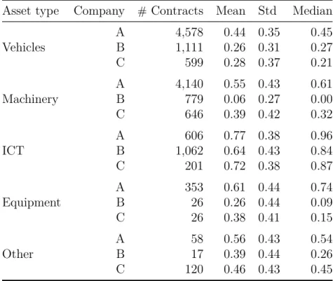
Previous studies on the LGD of defaulted leasing contracts consistently show
that the LGD distribution depends largely on the underlying asset type. We cat-
egorize the contracts according to the underlying asset using five classes: vehicles,
machinery, information and communications technology (ICT), equipment, and
Asset type Company # Contracts Mean Std Median
Vehicles A 4,578 0 . 44 0 . 35 0 . 45
B 1,111 0 . 26 0 . 31 0 . 27 C 599 0 . 28 0 . 37 0 . 21
Machinery A 4,140 0 . 55 0 . 43 0 . 61
B 779 0 . 06 0 . 27 0 . 00 C 646 0 . 39 0 . 42 0 . 32
ICT A 606 0 . 77 0 . 38 0 . 96
B 1,062 0 . 64 0 . 43 0 . 84 C 201 0 . 72 0 . 38 0 . 87
Equipment A 353 0 . 61 0 . 44 0 . 74
B 26 0 . 26 0 . 44 0 . 09
C 26 0 . 38 0 . 41 0 . 15
Other A 58 0 . 56 0 . 43 0 . 54
B 17 0 . 39 0 . 44 0 . 26
C 120 0 . 46 0 . 43 0 . 45
Table 2.3: Loss given default (LGD) density information by asset type for companies A–C. For each asset type, # Contracts is the number of contracts containing this type of asset, Mean is its mean, Std is its standard deviation, and Median is its median. ICT is information and communications technology. The displayed asset types vary in the numbers of their contracts and even further in the characteristics of their realized LGD.
other. Table 2.3 summarizes the key statistical figures of the distributions for each company. We can unambiguously rank the three companies with respect to their mean LGD. Company B achieves the lowest average LGD for all asset types, company C is second best, and company A bears the highest losses. Contracts in ICT have the highest average LGD. Examining the median of ICT, we find that companies A, B, and C retrieve only 4%, 16%, and 13% of the EAD, respectively, in half of the cases. The key statistical figures for equipment and other assets are seemingly less meaningful because of the small sample sizes for these classes, but the trends are consistent across all three companies.
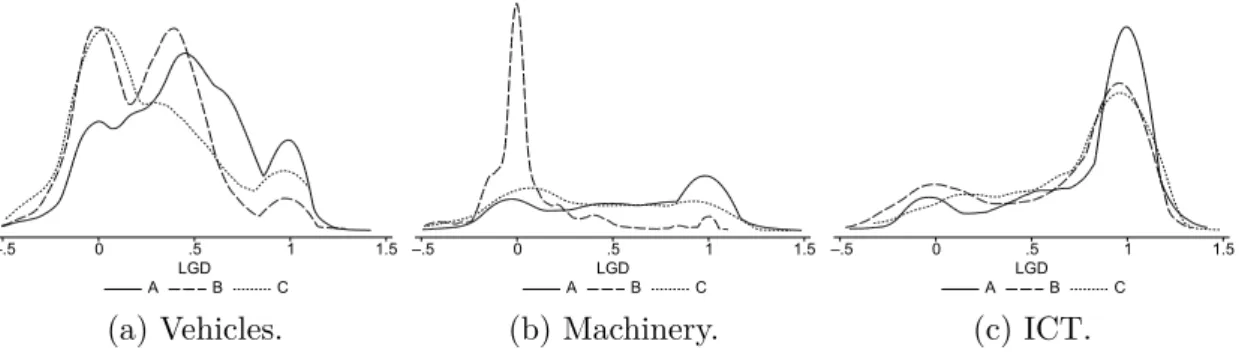
Figure 2.2 presents the LGD distributions for vehicles, machinery, and ICT for
each company. The shape of the LGD distributions differs tremendously with
respect to the different asset types. Whereas for ICT, the LGD density in Fig-
–.5 0 .5 1 1.5
A LGDB C
(a) Vehicles.
–.5 0 .5 1 1.5
A LGDB C
(b) Machinery.
–.5 0 .5 1 1.5
A LGDB C