Advanced Methods for
Loss Given Default Estimation
Inauguraldissertation zur
Erlangung des Doktorgrades der
Wirtschafts- und Sozialwissenschaftlichen Fakultät der
Universität zu Köln 2015
vorgelegt von
Dipl.-Wirt.-Math. Eugen Töws
Klimowka aus
Referent: Univ.-Prof. Dr. Thomas Hartmann-Wendels, Universität zu Köln Korreferent: Univ.-Prof. Dr. Dieter Hess, Universität zu Köln
Vorsitz: Univ.-Prof. Dr. Heinrich R. Schradin, Universität zu Köln
Tag der Promotion: 11. Januar 2016
Acknowledgments
The completion of this thesis would not have been possible without the support from many people, whom I would like to thank.
Foremost, I would like to express my sincere gratitude to my advisor Professor Dr. Thomas Hartmann-Wendels for his continuous support, patience, motivation, and immense knowledge. His guidance helped me in all the time of research and writing of this thesis. I would also like to thank him for the opportunity to present my work at several international conferences. Further thanks go to Professor Dr. Dieter Hess for serving as co-referee and Professor Dr. Heinrich Schradin for chairing the dissertation committee.
I am greatly indebted to Patrick Miller, who partnered with me on the the- sis’ subject from the first day. I am especially grateful for the numerous highly productive discussions with him that resulted in two co-authored projects. I very much appreciate conducting joint research with him. I want to thank Dr. Hans Elbracht for his exceptional work on collecting the data employed in this thesis without which this thesis would not have been.
Many thanks go to my former colleagues at the University of Cologne. In particular, I would like to mention Patrick Wohl, Dr. Tobias Schlüter, Dr. Claudio Wewel, Benjamin Döring, David Fritz, and Elke Brand as well as Dr. Claudia Wendels and Dr. Wolfgang Spörk for their advice and support concerning matters beside this thesis. I am grateful for the wonderful time spent together both on and off campus.
Finally, I wish to thank my mother Irene and above all my girlfriend Genesis for her steady encouragement and support that made the completion of this work possible and who continuously reminded me of the really important things in life.
Cologne, January 2016 Eugen Töws
This thesis consists of the following works:
Thomas Hartmann-Wendels, Patrick Miller, and Eugen Töws, 2014. Loss given default for leasing: Parametric and nonparametric estimations. Journal of Banking & Finance 40, 364–375.
Eugen Töws, 2014. The impact of debtor recovery on loss given default. Working paper.
Patrick Miller and Eugen Töws, 2015. Loss given default-adjusted workout pro-
cesses for leases. Working paper.
Contents
List of Abbreviations xi
List of Figures xiii
List of Tables xiv
1 Introduction 1
2 Loss given default for leasing: Parametric and nonparametric
estimations 9
2.1 Literature review . . . . 11
2.2 Dataset . . . . 14
2.3 Methods . . . . 19
2.3.1 Finite mixture models and classification . . . . 20
2.3.2 Regression and model trees . . . . 22
2.3.3 Out-of-sample testing . . . . 25
2.4 Results . . . . 26
2.4.1 In-sample results . . . . 27
2.4.2 Out-of-sample results . . . . 29
2.4.3 Validation and interpretation . . . . 36
2.5 Conclusion . . . . 41
3 The impact of debtor recovery on loss given default 43
3.1 Dataset . . . . 46
3.2 Methods . . . . 52
3.2.1 Tree algorithms . . . . 53
3.2.2 Regression model . . . . 56
3.2.3 Model testing . . . . 56
3.3 Results . . . . 58
3.3.1 Recovery classification . . . . 59
3.3.2 Loss given default estimation . . . . 61
3.3.3 Validation and robustness . . . . 64
3.4 Conclusion . . . . 67
4 Loss given default-adjusted workout processes for leases 71
4.1 Dataset . . . . 76
4.2 Methods . . . . 83
4.2.1 Direct estimation . . . . 84
4.2.2 Loss given default decomposition . . . . 86
4.2.3 Loss given default classification . . . . 88
4.2.4 Validation techniques . . . . 89
4.2.5 Performance measurements . . . . 93
4.3 Results . . . . 94
4.3.1 In-sample validation . . . . 95
4.3.2 Out-of-sample validation . . . . 96
4.3.3 Out-of-time validation . . . . 98
4.3.4 Further estimation and classification . . . 100
4.3.5 Interpretation . . . 103
4.4 Conclusion . . . 107
5 Summary and conclusion 109
Bibliography 111
List of Abbreviations
AIC Akaike information criterion ALGD Asset-related loss given default AP Asset proceeds
ARR Asset-related recovery rate BIC Bayesian information criterion
CF Cash flows
CRR Capital requirement regulation EAD Exposure at default
FMM Finite mixture model
ICT Information and communications technology IRBA Internal ratings based approach
Is In-sample
k
NN
k-nearest neighbor LC Liquidation costs LGD Loss given default MAE Mean absolute error
MLGD Miscellaneous loss given default MRR Miscellaneous recovery rate MSE Mean squared error
MURD Moody’s Ultimate Recovery Database
NN Neural network
OLS Ordinary least squares Oos Out-of-sample
Oot Out-of-time
PD Probability of default
RF Random forest
RMSE Root mean squared error
RR Recovery rate
RT Regression Tree
SVM Support vector machine
TARGET Tree analysis with randomly generated and evolved trees TIC Theil inequality coefficient
WC Workout costs
List of Figures
2.1 Density of realized loss given default by company. . . . 17 2.2 Density of realized loss given default by company for the three
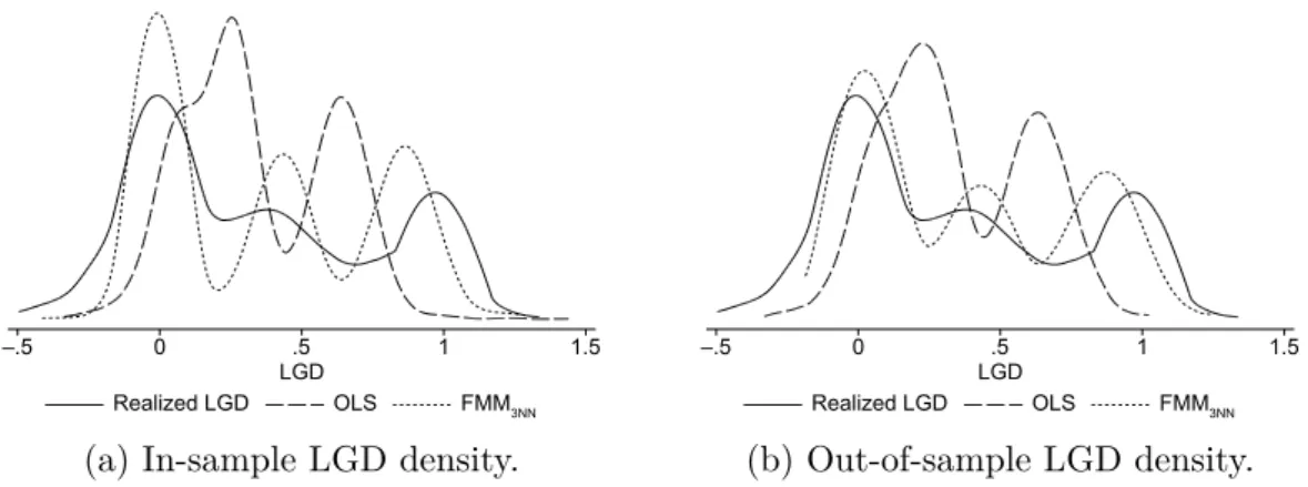
major asset types: vehicles, machinery, and information and com- munications technology. . . . 19 2.3 Densities of realized loss given default, loss given default estimated
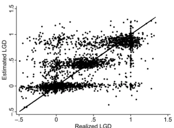
by ordinary least squares regression without variable selection, and loss given default estimated by finite mixture combined with 3- nearest neighbors for company B. . . . 37 2.4 Scatter plot of realized and in-sample and out-of-sample estimated
loss given default. . . . 38 3.1 Density of loss given default of the total dataset and recovered and
written off contracts of companies D–F. . . . 51 3.2 Procedure of the two-step model. . . . 53 3.3 Receiver operating characteristic curves for random forest classifi-
cation of company D’s dataset at contracts’ default. . . . 65 3.4 Out-of-sample classification error for random forest classification of
company D’s recovered and written off contracts as a function of the forest’s size. . . . 68 4.1 Densities of loss given default, after separating the contracts ac-
cording to their relationship of loss given default to asset-related loss given default. . . . 80 4.2 Density of loss given default, asset-related loss given default, and
miscellaneous loss given default. . . . 81
4.3 Procedure of the developed models. . . . 85
4.4 Validation techniques. . . . 90
4.5 Visual comparison of realized and estimated loss given default. . . 104
2.1 Numbers of contracts and lessees in the datasets of companies A–C in descending order of the number of contracts. . . . 14 2.2 Loss given default density information for companies A–C. . . . . 16 2.3 Loss given default density information by asset type for companies
A–C. . . . 18 2.4 In-sample estimation errors at the execution and default of con-
tracts by company. . . . 28 2.5 Out-of-sample estimation errors at the execution and default of
contracts by company. . . . 30 2.6 Out-of-sample estimation errors at the execution and default of
contracts by sample size. . . . 34 2.7 Janus quotient for in-sample and out-of-sample estimations of loss
given default for each method and company at execution and de- fault of the contracts. . . . 35 2.8 In-sample classification errors for the 3-nearest neighbors and J4.8
methods at execution and default of the contracts. . . . 39 3.1 Number of contracts and lessees in the datasets of companies D–F
in descending order of the most current default year. . . . 47 3.2 Categorized information contained in the datasets of companies D–F. 48 3.3 Loss given default density information of recovered and written off
contracts for companies D–F. . . . 49 3.4 Classification errors at execution and default of the contracts of
companies D–F. . . . 59 3.5 Coefficient of determination
R2of the one-step and two-step models
for companies D–F. . . . 62 3.6 Variable importance in random forest for company D’s contracts at
their default. . . . 67
4.1 Distribution parameters of loss given default. . . . 79
4.2 Distribution parameters of loss given default for each default year. 82
4.3 Year of default and frequency of contracts. . . . 92
List of Tables xv 4.4 In-sample loss given default estimation results. . . . 96 4.5 Out-of-sample loss given default estimation results. . . . 97 4.6 Out-of-time loss given default estimation results. . . . 99 4.7 Asset-related loss given default and miscellaneous loss given default
estimation results. . . 101 4.8 Classification results of classifying according to Equation (4.7). . . 102 4.9 Classification results of classifying according to Equation (4.7), con-
sidering exclusively classification probabilities below 25% or above 75%. . . 103 4.10 Comparison of performance improvements in loss given default es-
timation literature. . . 106
1 Introduction
Credit risk is a major concern of financial institutions and their risk management.
To the institutes, it is essential to identify and measure this risk in order to make economically reasonable credit decisions and to calculate regulatory capital. For the determination of credit risk of financial assets, banking regulation provides three essential components. These are the probability of default (PD), the loss given default (LGD), and the exposure at default (EAD). Moreover, two different approaches are provided to incorporate these components. Article 107 (1) of the capital requirement regulation (CRR) states that financial institutions shall apply either the Standardised Approach or the Internal Ratings Based Approach (IRBA) to calculate their regulatory capital requirements for credit risk. Depending on the chosen approach, these components can or must be determined for regulatory and economic purposes. With the IRBA, the Basel Committee on Banking Supervision (2003) intends to increase the sensitivity of risk factors to the risk of the assets of the applying institutions. A risk-adequate approach, such as IRBA, should ideally reduce the regulatory capital of these institutes. Consequently, capital could be released that is tied-up in backing financial assets.
So far, researchers studied the PD extensively and established sophisticated
measurements, such as the value-at-risk. Implementations are available abun-
dantly, e. g., CreditPortfolioView, CreditMetrics
TM, and
CreditRisk+. Front-
czak and Rostek (2015) assume that the EAD is predictable to a large extent by
means of amortization schedules. Hence, only for LGD robust estimation proce-
dures are scarce.
In the following, we will consider LGD in more detail. LGD is that share of the outstanding claim of a defaulted contract that could not have been recovered.
Several studies refer to its counterpart the recovery rate, which is 1
−LGD.
Accurate estimates of potential losses are essential to allocate economic and regulatory capital and to price credit risk of financial instruments. Moreover, Gürtler and Hibbeln (2013) argue that accurately estimating the LGD should re- sult in competitive advantages to the applying institution. Against this theoretical and practical background, this thesis contributes to the growing research area of LGD estimation. Particularly, it introduces new approaches and puts these into the context of the existing literature. Furthermore, several findings in related research can be confirmed empirically or put into perspective.
Recent studies on the estimation of LGD are mainly based on defaulted loans and bonds, such as Yao et al. (2015), Leow et al. (2014), Jankowitsch et al.
(2014), Khieu et al. (2011), and Calabrese and Zenga (2010). Only little evidence
exists on the LGD of leases apart from Hartmann-Wendels and Honal (2010),
De Laurentis and Riani (2005), and Schmit and Stuyck (2002). However, there is
at least one major peculiarity of leases when comparing their recovery risk to that
of loans, which may reduce the LGD significantly. Eisfeldt and Rampini (2009)
argue that for the legal owner of the leased asset, i. e. the lessor, its reposition is
easier than foreclosure on the collateral for a secured loan. Moreover, the lessor
may retain any value from disposing of the asset, even if the recoveries exceed the
outstanding claim. Thus, the asset of a lease contract is a native collateral, which
lessors are experts in disposing off. In fact, examining defaulted lease contracts
from major European financial institutions, Schmit and Stuyck (2002) find that
defaulted leases on vehicles and real estate on average exhibit lower LGDs than
loans and bonds. Theoretically, this finding is plausible. However, there might be
exceptions to this rule.
3
Calculation of LGD is a rather technical issue. There are two acknowledged methods to determine the LGD of financial instruments. One of which is the concept of market LGDs. The market LGD is calculated as one minus the ratio of the trading price of the asset some time after default to the trading price at the time of default. However, market LGDs are only available for bonds and loans issued by large firms. Moreover, Khieu et al. (2011) find evidence, that market LGDs are biased and inefficient estimates of the realized LGD. The second concept is the workout LGD. Workout LGDs are calculated as one minus the ratio of the discounted cash flows after default to the EAD.
The distribution of workout LGDs is often reported to be bimodal, e. g. by Li et al. (2014), Qi and Zhao (2011), and Hartmann-Wendels and Honal (2010). The distribution of a parameter is considered bimodal if it exhibits two local maxima.
Particularly for the LGD of leases these maxima are located around zero and one.
This shape is rather unusual because there is no single probability function com- ing close to bimodal distributions. The unusual shape raises the question whether standard econometric methods, such as ordinary least squares (OLS) linear re- gression, are appropriate for the estimation task. This thesis presents empirical evidence that complex approaches, such as regression trees and multi-step models, have a significant advantage over standard methods, given a sufficiently large data and information base. Furthermore, we find that economic consideration can be a key driver of estimation improvements.
All approaches developed in this work incorporate workout LGDs and several additional requirements of the CRR and its predecessor Basel II. In particular, we consider workout costs and the update of LGD estimates in case of default, which prior literature mostly neglects.
This thesis consists of three essays on the estimation of the risk parameter LGD.
The first essay (Hartmann-Wendels, Miller, and Töws, 2014, Loss given default
for leasing: Parametric and nonparametric estimations) fills a gap in LGD re- lated literature by focusing on elementary differences of the examined estimation approaches. Three major German leasing companies provided a total of 14
,322 defaulted leasing contracts. Based on this data, we compare parametric, semi- parametric and nonparametric estimation methods. We use the historical average and the parametric OLS regression as benchmark and compare the semipara- metric finite mixture model (FMM) to the nonparametric model tree M5'. We evaluate the performance of the used methods in an in-sample and out-of-sample validation.
The most elementary estimation method is a look-up table, which either bases on historical averages or expert opinions (see Gupton and Stein (2005)). Directly following is OLS, which is also easy to implement. Therefore, OLS dominates the used methods for estimating the LGD in recent literature. Most empirical studies find the LGD to have a bimodal or even multimodal shape. Given this finding, OLS may lead to inefficient estimates by estimating the conditional expectation of the LGD. Whereas it is econometrically reasonable to approximate the LGD distribution by a mixture of a finite number of standard distributions, e. g. normal distributions. Implementing FMM, we develop a multi-step model to cluster the data into distinct clusters first. The data then is classified to the found clusters employing different classification algorithms. Finally, we calibrate OLS models to the contracts of each cluster. Thereby, we allow for different influencing factors within these clusters. The last category of studied approaches is tree algorithms.
These methods produce decision trees using if-then conditions to divide the data subsequently in order to reduce its inhomogeneity. The determined final subsam- ples then are averaged in terms of their LGD. Alternatively, regression models are built within these subsamples.
Our results show that a model’s in-sample performance is a poor indicator
of its out-of-sample estimation capability. We find that FMM is quite capable
5
of reproducing the unusual shape of the LGD distribution in-sample as well as out-of-sample. Moreover, when measuring the models performance in terms of the deviation of estimated from realized LGDs, FMM produces very low in-sample er- rors. However, out-of-sample the error increases significantly and exceeds that of OLS in most cases. While OLS is mostly outperformed in-sample, the model tree produces robust in-sample and out-of-sample estimations exhibiting the lowest level of out-of-sample estimation errors. Furthermore, we find that the improve- ment of the model tree increases with an increasing dataset. Also, all models’
performance level is highly dependent on the peculiarities of the underlying data.
In order to account for a company’s idiosyncratic characteristics, it is reasonable to consider the datasets separately.
The second essay (Töws, 2014, The impact of debtor recovery on loss given default) addresses the economic consideration of the workout process of defaulted contracts. It founds on the lessor’s retainment of legal title to the leased asset and, consequently, his easy access to it in case of default. Dependent on the lessor’s workout strategy, defaulted contracts may develop in two distinct ways. Either the default reason can be dissolved and the debtor recovers or the contract must be written off. This work uses the essential information of the contract’s default end to study its influence on the LGD. We observe the recovery or write-off of 42
,575 defaulted leasing contracts of three German leasing companies. In the data, we find that recovered contracts exhibit significantly lower LGD levels than contracts that were written off. According to the significant influence, we provide evidence that employing the default end in an LGD estimation approach is highly beneficial to the estimation accuracy.
Reminding ourselves that regression trees performed well in estimating LGD in the first essay, we compare the forecasting performance of three tree algorithms.
These are J4.8, random forest (RF), and C5.0. Developing a two-step approach
for estimating LGD, we first divide the data according to the contracts’ default
end in a classification. On each of the two classes, a regression model is calibrated in the second step, and every contract is assigned exactly two LGD estimations from both of the regression models. The final LGD estimation then is the linear combination of the estimated LGDs weighted with their respective classification probability.
Compared to direct estimation with OLS, we find our approach to improve the estimation accuracy of LGD. When we consider the coefficient of determination, the improvement is significant for each of the three datasets. The study indicates the benefits of establishing the lessor’s expertise in assessing a defaulted contract’s continuation worthiness. If successfully implemented, the resulting workout pro- cess should produce lower LGDs than before and thereby strengthen the lenders competitiveness.
The third essay (Miller and Töws, 2015, Loss given default-adjusted workout processes for leases) contributes to the LGD estimation literature considering unique features of leasing contracts. Based on a dataset of 1
,493 defaulted leasing contracts, we economically account for leasing peculiarities and develop a partic- ularly suited approach to estimate the contracts’ LGD. To the best of our knowl- edge, we are the first to separate the LGD into two distinct parts. We ground this separation on the economic consideration that cash flows of the workout process of defaulted leasing contracts, in general, are coming from two distinct sources.
The first part includes all asset-related cash flows, such as the asset’s liquidation value and incurred liquidation costs. The second part comprises the remaining cash flows, such as overdue payments and collection costs.
In the course of the study, we find ALGD to be a theoretical upper bound to
the LGD, given that the MLGD does not exceed a value of one. Assuming this is
the case, an ALGD less than one directly indicates the overall LGD being below
a value of one. As soon as ALGD reaches a value of zero, the disposal revenues
7 cover EAD in full. In any case, if MLGD exceeds a value of one, the lessor should restrict the workout process to the asset’s disposal. Under such circumstances, the collection of overdue payments is economically inefficient and causes monetary losses to the lessor.
Constructing a multi-step LGD estimation approach, we essentially compare the performance of two different methods: OLS regression and RF. The first step estimates the respective shares of the LGD. These are the asset-related LGD (ALGD) and the miscellaneous LGD (MLGD). Including these factors, we perform a classification of the data in the second step. We estimate whether a contract’s ALGD exceeds its LGD. Similar to the approach of the second essay, we calibrate regression models for each class in step three. The final LGD estimation is the weighted linear combination of the estimated LGDs and the contract’s classification probability.
Including the estimated ALGD and MLGD into the estimation approach in-
creases the estimation accuracy. Most importantly, the relative performance im-
provement is independent of the method applied. It rather arises from the eco-
nomic approach, which targets the specifics of leasing contracts. We find that the
estimated values of ALGD and MLGD are sturdy indicators for the success or
failure of the workout process. Thus, the lessor can benefit from the consideration
of both these forecasts for his actions concerning the workout process.
2 Loss given default for leasing:
Parametric and nonparametric estimations
The loss given default (LGD) and its counterpart, the recovery rate, which equals one minus the LGD, are key variables in determining the credit risk of a financial asset. Despite their importance, only a few studies focus on the theoretical and empirical issues related to the estimation of recovery rates.
Accurate estimates of potential losses are essential to efficiently allocate regu- latory and economic capital and to price the credit risk of financial instruments.
Proper management of recovery risk is even more important for lessors than for banks because leases have a comparative advantage over bank loans with respect to the lessor’s ability to benefit from higher recovery rates in the event of default.
In their empirical cross-country analysis, Schmit and Stuyck (2002) note that the average recovery rate for defaulted automotive and real estate leasing contracts is slightly higher than the recovery rates for senior secured loans in most countries and much higher than the recovery rates for bonds. Moreover, the recovery time for defaulted lease contracts is shorter than that for bank loans. Because the lessor retains legal title to the leased asset, repossession of a leased asset is easier than foreclosure on the collateral for a secured loan. Moreover, the lessor can retain any recovered value in excess of the exposure at default. Repossessing used assets and maximizing their return through disposal in secondary markets are aspects of normal leasing business and are not restricted to defaulted contracts.
Therefore, lessors have a good understanding of the secondary markets and of the
assets themselves. Because the lessor’s claims are effectively protected by legal ownership, the high recoverability of the leased asset may compensate for the poor creditworthiness of a lessee. Lasfer and Levis (1998) find empirical evidence for the hypothesis that lower-rated and cash-constrained firms have a greater propen- sity to become lessees. To leverage their potential lower credit risk, lessors must be able to accurately estimate the recovery rates of defaulted contracts.
This paper compares the in-sample and out-of-sample accuracies of parametric and nonparametric methods for estimating the LGD of defaulted leasing contracts.
Employing a large dataset of 14
,322 defaulted leasing contracts from three major German lessors, we find in-sample accuracy to be a poor predictor of out-of-sample accuracy. Methods such as the hybrid finite mixture models (FMMs), which at- tempt to reproduce the LGD distribution, perform well for in-sample estimation but yield poor results out-of-sample. Nonparametric models, by contrast, are ro- bust in the sense that they deliver fairly accurate estimations in-sample, and they perform best out-of-sample. This result is important because out-of-sample esti- mation has rarely been performed in other studies – with the notable exceptions of Han and Jang (2013) and Qi and Zhao (2011) – although out-of-sample accuracy is critical for proper risk management and is required for regulatory purposes.
Analyzing estimation accuracy separately for each lessor, our results suggest that the number of observations within a dataset has an impact on the relative performance of the estimation methods. Whereas sophisticated nonparametric estimation techniques yield, by far, the best results for large datasets, simple OLS regression performs fairly well for smaller datasets.
Finally, we find that estimation accuracy critically depends on the available
set of information. We estimate the LGD at two different points in time, at the
execution of the contract and at the point of contractual default. This procedure
is of particular importance for leasing contracts because the loan-to-asset value
changes during the course of a leasing contract. Furthermore, the Basel II accord
2.1 Literature review 11 requires financial institutions using the advanced internal ratings based approach (IRBA) to update their LGD estimates for defaulted exposure. To the best of our knowledge, an analysis of this type of update has been neglected in the literature thus far.
2.1 Literature review
There are two major challenges in estimating recovery rates for leases with respect to defaulted bank loans or bonds. First, estimates of LGD on loans or bonds take for granted that the recovery rate is bounded within the interval [0
,1], which assumes that the bank cannot recover more than the outstanding amount (even under the most favorable circumstances) and that the lender cannot lose more than the outstanding amount (even under the least favorable circumstances). Although the assumption of an upper boundary is justified for bank loans, it does not apply to leasing contracts. As the legal owner of the leased asset, the lessor may retain any value recovered by redeploying the leased asset, even if the recoveries exceed the outstanding claim. In fact, there is some empirical evidence that recovery rates greater than 100% are by no means rare. For example, Schmit and Stuyck (2002) report that up to 59% of all defaulted contracts in their sample have a recovery rate that exceeds 100%. Using a different dataset, Laurent and Schmit (2005) find that recovery rates are greater than 100% in 45% of all defaulted contracts.
The lower boundary of the recovery rate rests on the implicit assumption of a
costless workout procedure. In fact, most empirical studies neglect workout costs
(presumably) because of data limitations. Only Grippa et al. (2005) account for
workout costs in their study of Italian bank loans and find that workout costs
average 2
.3% of total operating expenses. The Basel II accord, however, requires
that workout costs are included in the LGD calculation. Thus, when workout costs
are incorporated, there is no reason to assume that workout recovery rates must
be non-negative. The second challenge in estimating recovery rates is the bimodal
nature of the density function, with high densities near 0 and 1. This property of workout recovery rates is well documented in almost all empirical studies, whether of bank loans or leasing contracts (e. g., Laurent and Schmit (2005)).
Because of the specific nature of the recovery rate density function, standard econometric techniques, such as OLS regression, do not yield unbiased estimates.
Renault and Scaillet (2004) apply a beta kernel estimator technique to estimate the recovery rate density of defaulted bonds, but they find that it is difficult to model its bimodality. Calabrese and Zenga (2010) extend this approach by con- sidering the recovery rate as a mixed random variable obtained as a mixture of a Bernoulli random variable and a continuous random variable on the unit interval and then apply this new approach to a large dataset of defaulted Italian loans.
Qi and Zhao (2011) compare fractional response regression to other parametric and nonparametric modeling methods. They conclude that nonparametric meth- ods – such as regression trees (RTs) and neural networks – perform better than parametric methods when overfitting is properly controlled for. A similar result is obtained by Bastos (2010), who compares the estimation accuracy of fractional response to RTs and neural networks.
Despite the growing interest in the modeling of recovery rates, little empirical
evidence is available on this topic. Several studies (e. g., Altman and Ramayanam
(2007), Friedman and Sandow (2005), and Frye (2005)) rely on the concept of
market recoveries, which are calculated as the ratio of the price for which a de-
faulted asset is traded some time after default to the price of that asset at the time
of default. Market recoveries are only available for bonds and loans issued by large
firms. Workout recoveries are used by Khieu et al. (2011), Dermine and Neto de
Carvalho (2005), and Friedman and Sandow (2005). However, Khieu et al. (2011)
find evidence that the post-default price of a loan is not a rational estimate of
actual recovery realization, i. e., it is biased and/or inefficient. According to Frye
(2005), many analysts prefer the discounted value of all cash flows as a more re-
2.1 Literature review 13 liable measurement of defaulted assets because: (1) cash flows ultimately become known with certainty, whereas the market price is derived from an uncertain fore- cast of future cash flows; (2) the market for defaulted assets might be illiquid; (3) the market price might be depressed; and (4) the asset holder might not account for the asset on a market-value basis.
Schmit et al. (2003) analyze a dataset consisting of 40
,000 leasing contracts, of which 140 are defaulted. Using bootstrap techniques, they conclude that the credit risk of a leasing portfolio is rather low because of its high recovery rates.
Similar studies are conducted by Laurent and Schmit (2005) and Schmit (2004).
Schmit and Stuyck (2002) find considerable variation in the recovery rates of 37
,000 defaulted leasing contracts of 12 leasing companies in six countries. Aver- age recovery rates depend on the type of the leased asset, country, and contract age. De Laurentis and Riani (2005) find empirical evidence that leasing recov- ery rates are inversely correlated with the level of exposure at default. However, recovery rates increase with the original asset value, contract age, and existence of additional bank guarantees. Applying OLS regressions to forecast LGDs in that study leads to rather poor results: the unit interval is divided into three equal intervals, and only 31–67% of all contracts are correctly assigned in-sample.
With a finer partition of five intervals, the portion of correctly assigned contracts decreases even further. These results clearly indicate that more appropriate esti- mation techniques are needed to accurately estimate recovery rates.
Our study differs from the LGD literature in several crucial aspects. First, we
calculate workout LGDs and consider workout costs. Second, we perform out-
of-sample testing at contract execution and default, which meets the Basel II
requirements for LGD validation. Third, by separately analyzing the datasets of
three lessors, we gain insight into the robustness of the estimation techniques.
Company
#Contracts
#Lessees
A 9
,735 5
,811
B 2
,995 2
,344
C 1
,592 964
Table 2.1: Numbers of contracts and lessees in the datasets of companies A–C in de- scending order of the number of contracts.
2.2 Dataset
This study uses datasets provided by three German leasing companies, which shall be referred to herein as companies A, B, and C. All three companies use a default definition consistent with the Basel II framework. According to Table 2.1, the dataset from lessor A contains 9
,735 leasing contracts with 5
,811 different customers and default dates between 2002 and 2010. The dataset from lessor B contains 2
,995 leasing contracts with 2
,344 different lessees who defaulted between 1994 and 2009, with the majority of defaults occurring between 2001 and 2008.
The dataset for leasing company C consists of 1
,592 leasing contracts with 864 different lessees who defaulted between 2002 and 2009.
For the defaulted contracts, we calculate the LGD as one minus the recovery rate. The recovery rate is the ratio of the present value of cash inflows after default to the exposure at default (EAD). For leasing contracts, the cash flows consist of the revenues obtained by redeploying the leased asset and other collat- eral combined with other returns and less workout expenses. The cash flows are discounted to the time of default using the term related refinancing interest rate.
1The EAD is the sum of the present value of the outstanding minimum lease pay- ments, compounded default lease payments, and the present residual value. All values refer to the time of default. A contract is classified as defaulted when at least one of the triggering events set out in the Basel II framework has occurred.
1Only a few studies (such as Gibilaro and Mattarocci (2007)) address risk-adjusted discounting.
We use the term related refinancing interest rate to discount cash flows at the time of default, independently of the time span of the workout and the risk of each type of cash flow.
2.2 Dataset 15 Before the data was collected, all three companies agreed to use identical defi- nitions for all the elements that are entered into the LGD calculation, and for all details of the leasing contract, lessee, and leased asset. Thus, for every contract, we have detailed information about the type and date of payments that the lessor received after the default event. Moreover, we incorporate expenses arising during the workout into the LGD calculation, to meet Basel II requirements. Workout costs are rarely considered in empirical studies.
The workouts have been completed for all the observed contracts. Gürtler and Hibbeln (2013) recommend restricting the observation period of recovery cash flows to avoid the under-representation of long workout processes, which might result in an underestimation of LGDs. Because we do not see a similar problem in our data, we do not truncate our observations based on that effect.
All three companies also provide a great deal of information about factors that might influence the LGD, which we divide into four categories:
1. contract information;
2. customer information;
3. object information; and
4. additional information at default.
Contract information is elementary information about the contract, such as its type, e. g., whether it was a full payment lease, partial amortization, or hire- purchase; its duration; its calculated residual value or prepayment rents; and in- formation about collateralization and/or purchase options. Customer information mainly identifies retail and non-retail customers. The category object information consists of basic information about the object of the lease, including its type, ini- tial value, and supplementary information, such as the asset depreciation range.
Whereas all the information in the first three groups is available from the moment
the contract is concluded, the last category consists of information that only be-
Company Mean Std P5 P25 Median P75 P95 A 0
.52 0
.40
−0
.11 0
.19 0
.52 0
.88 1
.05 B 0
.35 0
.42
−0
.18 0
.00 0
.25 0
.72 1
.01 C 0
.39 0
.42
−0
.23 0
.03 0
.32 0
.77 1
.03
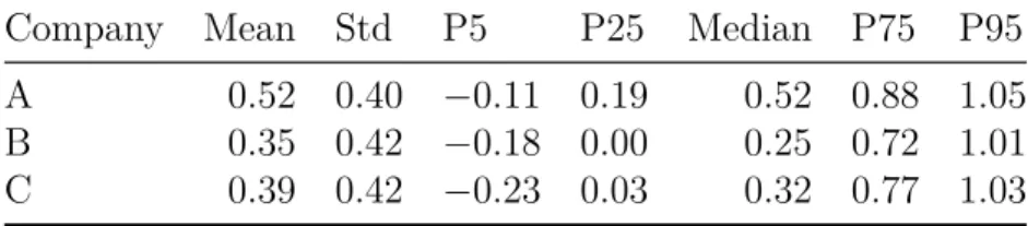
Table 2.2: Loss given default (LGD) density information for companies A–C. Std is the standard deviation and P5–P95 are the respective percentiles.
comes available after the contract has defaulted, such as the exposure at default and the contract age at default.
Descriptive statistics
The LGD is clearly not restricted to the interval [0
,1]. As presented in Table 2.2 and Figure 2.1, negative LGDs are not only theoretically possible but also occur frequently in the leasing business. Hartmann-Wendels and Honal (2010) argue that such cases mainly occur if a defaulted contract with a rather low EAD yields a high recovery from the sale of the asset. Because we incorporate the workout expenses, LGDs greater than one are also feasible. Thus, we do not bound LGDs within the [0
,1] interval, as is common for bank loans and as is done by Bastos (2010), by Calabrese and Zenga (2010), and by Loterman et al. (2012).
An LGD of 45%, as specified in the standard credit risk approach, is consider-
ably higher than the median LGDs observed for companies B and C. In general,
we emphasize that the shape of the LGD distribution varies significantly among
these three companies. As presented in Figure 2.1, only the LGD distribution of
company C exhibits the frequently mentioned bimodal shape, whereas those of
companies A and B feature three maxima. These differences continue to prevail
when we account for differences in the leasing portfolio. Thus, we trace these vari-
ations back to differences in workout policies. Because the requirements for the
pooling of LGD data, set out in section 456 of the Basel II accord, are clearly vio-
2.2 Dataset 17
–.5 0 .5 1 1.5
A LGD B C
Figure 2.1: Density of the realized loss given default (LGD) by company. The realized LGD concentrates on the interval [−0.5,1.5]. The figures describe a loss severity of
−50% on the left end, which indicates that 150% of the exposure at default (EAD) was recovered. On the right end, the loss severity is 150%, indicating a loss of 150% of the EAD. Consequently, a realized LGD of 0 or 1 indicates the following: in case of 0, full coverage of the EAD (included workout costs); or, in case of 1, total loss of the EAD.
lated, we construct individual estimation models to account for institution-specific characteristics and differences in LGD profiles among the companies.
Previous studies on the LGD of defaulted leasing contracts consistently show
that the LGD distribution depends largely on the underlying asset type. We cat-
egorize the contracts according to the underlying asset using five classes: vehicles,
machinery, information and communications technology (ICT), equipment, and
other. Table 2.3 summarizes the key statistical figures of the distributions for
each company. We can unambiguously rank the three companies with respect to
their mean LGD. Company B achieves the lowest average LGD for all asset types,
company C is second best, and company A bears the highest losses. Contracts in
ICT have the highest average LGD. Examining the median of ICT, we find that
companies A, B, and C retrieve only 4%, 16%, and 13% of the EAD, respectively,
in half of the cases. The key statistical figures for equipment and other assets are
Asset type Company
#Contracts Mean Std Median
Vehicles A 4,578 0
.44 0
.35 0
.45
B 1,111 0
.26 0
.31 0
.27 C 599 0
.28 0
.37 0
.21
Machinery A 4,140 0
.55 0
.43 0
.61
B 779 0
.06 0
.27 0
.00 C 646 0
.39 0
.42 0
.32
ICT A 606 0
.77 0
.38 0
.96
B 1,062 0
.64 0
.43 0
.84 C 201 0
.72 0
.38 0
.87
Equipment A 353 0
.61 0
.44 0
.74
B 26 0
.26 0
.44 0
.09
C 26 0
.38 0
.41 0
.15
Other A 58 0
.56 0
.43 0
.54
B 17 0
.39 0
.44 0
.26
C 120 0
.46 0
.43 0
.45
Table 2.3: Loss given default (LGD) density information by asset type for companies A–C. For each asset type, #
Contracts is the number of contracts containing this type of asset, Mean is its mean, Std is its standard deviation, and Median is its median. ICT is information and communications technology. The displayed asset types vary in the numbers of their contracts and even further in the characteristics of their realized LGD.
seemingly less meaningful because of the small sample sizes for these classes, but the trends are consistent across all three companies.
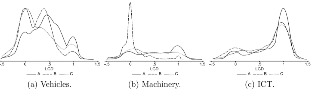
Figure 2.2 presents the LGD distributions for vehicles, machinery, and ICT for each company. The shape of the LGD distributions differs tremendously with respect to the different asset types. Whereas for ICT, the LGD density in Fig- ure 2.2c is right-skewed toward high LGDs with only weak bimodality throughout all of the companies, the density of machinery runs partly the opposite direction.
For machinery, in Figure 2.2b, we see a higher concentration around 0, but for
company A, larger LGDs again outweigh this effect. The LGD for contracts with
vehicles varies greatly from company to company. We observe a strong multi-
modality for all of the companies with an additional peak at approximately 0
.5,
and most of the density lies in the lower LGD range.
2.3 Methods 19
–.5 0 .5 1 1.5
A LGDB C
(a) Vehicles.
–.5 0 .5 1 1.5
A LGDB C
(b) Machinery.
–.5 0 .5 1 1.5
A LGDB C
(c) ICT.
Figure 2.2: Densities of realized loss given default (LGD) by company for the three major asset types: vehicles, machinery, and information and communications technology (ICT). Depending on the asset type, the realized LGD density appears in completely different shapes. For machinery (Figure b), even the difference between companies is enormous.
2.3 Methods
This section describes the various approaches that we use to estimate the LGD and its density. According to section 448 of the Basel II regulations, institutes are required to base their estimations on a history of defaults and to consider all relevant data, information, and methods. Furthermore, a bank using the advanced IRBA must be able to break down its experience with respect to the probability of default (PD), LGD, and the IRBA conversion factor. This breakdown is to be based on the factors that are identified as drivers of the respective risk parameters.
The basic method used to identify these drivers is to partition the data ac- cording to a certain attribute (e. g., the type of object). Differences in the means of the partitions are then captured by setting the inducing factor as the driver.
The average value is then the (naive) estimator of the LGD for the corresponding
subclass. As Gupton and Stein (2005) note, this traditional look-up table ap-
proach is static and backward-looking, even if considerable variation is observed
in the LGD distributions for different types of objects. An alternative method of
verifying the impact of potential factors and developing an estimation model is to
conduct a regression analysis. Linear regressions always estimate the (conditional)
expectation of the target variable, but this average is not a reasonable parameter
under mixed distributions, so it is not an adequate approach from a statistical perspective. However, regression analyses for LGD estimation are successfully implemented by Bellotti and Crook (2012) and by Zhang and Thomas (2012).
Table 2.2 reports the median LGDs as 52%, 25%, and 32% for companies A, B, and C, respectively. Considering the LGD distribution in Figure 2.1, its het- erogeneity suggests that the overall portfolio is composed of several subclasses, which are less heterogeneous in terms of the LGD. This implies that each sub- class has its own characteristic LGD distribution. We use FMMs to reveal these unknown classes (cluster analysis), to fit a reasonable model to the data and to classify the observations into these classes. Furthermore, we apply two different regression/model tree algorithms to the data. These tree-based models also have the basic function of dividing the portfolio into homogeneous partitions; by con- trast to the FMMs, however, the number of subclasses is endogenously determined rather than exogenously specified.
At the end of this section, we present an overview of how to select the ex- planatory variables for tree-based methods. We also describe our methodology for out-of-sample testing.
2.3.1 Finite mixture models and classification
Modeling the probability density of realized LGDs as a mixed distribution allows us to use different potential LGD drivers for different clusters and to capture differences in the effects of these drivers on the LGD in various subclasses. We adapt an approach originally proposed by Elbracht (2011). FMMs are described by Frühwirth-Schnatter (2006).
The approach consists of three steps: (1) cluster the total dataset into finite
classes by finite mixture distributions using all available information; (2) classify
the dataset into the resulting classes using only the information available at the
2.3 Methods 21 execution or default of the contract by the
k-nearest neighbors (
kNN) or the classification tree algorithm J4.8; and (3) perform OLS regressions for each class.
Step (1) can be adjusted between the two extremes of nonparametric and para- metric modeling, thus providing a flexible method of data adaptation. We use normal distributions to construct the mixing distributions. We estimate unknown model parameters using the expectation maximization algorithm, which also pro- vides a probabilistic classification of the observations. The accuracy of classifica- tion step (2) can be measured for in-sample testing. However, in out-of-sample testing, the goal is to classify observations that do not belong to any class initially – because these objects are not part of the training sample used to form classes – into exactly one of the given classes.
We compare two different approaches to classifying contracts into previously established classes. The nonparametric
kNN approach assigns an observation to the class with the majority of its
knearest neighbors, whereas the distance between observations is determined as the Euclidean distance. This approach is described by Hastie et al. (2009). We also apply the tree algorithm J4.8 for classification.
The J4.8 algorithm generates pruned C4.5 revision 8 decision trees, as illustrated
by Witten et al. (2011) and originally implemented by Quinlan (1993). The
decision tree is constructed by dividing the sample according to certain threshold
values. The optimal split in terms of maximized gain ratio is performed until
additional splits yield no further improvement, or a minimum of instances per
subset is reached. Every partition results in a node. To prevent overfitting, we
prune back the fully developed tree to a certain level. According to Quinlan
(1993), these deleted nodes shall not contribute to the classification accuracy of
unseen cases.
2.3.2 Regression and model trees
RTs are classified as nonparametric and nonlinear methods. Similar to other regression methods, they can be applied to analyze the underlying dataset and to predict the (numeric) dependent variable. An essential difference between RTs and parametric methods, such as linear or logistic regressions, is that ex-ante no assumption is made concerning the distribution of the underlying data, and no functional relationship is specified.
These characteristics are particularly beneficial in case of LGD estimation be- cause it is typically not possible to describe the distribution of the LGD suitably with a single distribution, such as the normal distribution. In addition, the dis- tribution of the LGD varies significantly according to the underlying data. Thus, as described in Section 2.2, the LGD distributions of the three companies studied here are all multimodal, although there are appreciable differences between com- panies, such as the number of maxima. In particular, more types of distributions are observed for bank loans (for an overview, see Dermine and Neto de Carvalho (2005)).
The basic idea of regression and model trees is to partition the entire dataset into homogeneous subsets by a sequence of splits, which creates a tree consisting of logical if-then conditions. Starting with the root node of the tree that contains all instances of the underlying data, each leaf covers only a fraction of the data.
In an RT, the prediction of the dependent variable is given by a constant for all instances belonging to a leaf, typically defined as the average value of these instances. Model trees are an extension of RTs in the sense that the target vari- able of instances belonging to a leaf is estimated by a linear regression model.
Therefore, model trees are hybrid estimation methods combining RTs and linear
regression. Model trees are clearly applicable for LGD estimation because RTs
are successfully used in previous studies such as Bastos (2010) and Qi and Zhao
(2011). Linear regression models are also applied to analyze and predict LGDs,
2.3 Methods 23 and these models may deliver comparable or better results than those of more complex models, as shown by Bellotti and Crook (2012) and Zhang and Thomas (2012).
For our LGD estimation, we apply the M5' model tree algorithm and the cor- responding RT algorithm that is introduced by Wang and Witten (1997) and described by Witten et al. (2011). This algorithm is a reconstruction of Quinlan’s M5 algorithm that was published in 1992. In the case of the M5' algorithm, the underlying dataset is divided step by step, each time using the binary split based on the explanatory variables with the greatest expected reduction in the stan- dard deviation. The constructed tree is subsequently pruned back to obtain an appropriately sized tree to control overfitting, which can influence out-of-sample performance negatively.
The resulting tree essentially depends on the explanatory variables used, par- ticularly with respect to the M5' model tree algorithm; selecting appropriate vari- ables is a complex issue because of ex-ante relevance and effectiveness not always being known. In the first step, we consider the potential application of a large number of parameters. However, it might be preferable to include only a fraction of the available variables, which we account for in the second step.
There are various algorithmic approaches for variable selection; two frequently applicable greedy algorithms are forward selection and backward elimination. Bel- lotti and Crook (2012) use forward selection for their LGD estimations of retail credit cards with OLS regression. However, forward selection has a significant disadvantage neglecting variable interactions.
Instead of forward selection, we employ backward elimination, initiating all
available variables and step by step eliminating the variables without which the
best value in terms of the respective fit criterion is achieved. This procedure
continues until a stop condition is reached, or all the variables are eliminated.
A typical fit criterion for regression models is the F-score. However, the Akaike information criterion (AIC) and Bayesian information criterion (BIC) are used for forecasting, both of which are based on the log-likelihood function.
Analogous to the approximation of the AIC used by Bellotti and Crook (2012), the BIC can be approximated by
BIC =
n·ln(MSE) +
p·ln(
n)
,(2.1)
where
ndenotes the number of observations,
pis the number of input variables, and MSE is the mean squared error of the observations.
We use the BIC, which penalizes the complexity of the model more than the AIC. This complexity is measured by the number of input variables. In addition to the number of explanatory variables, regression and model trees offer another complexity feature: the number of leaves in the computed tree. This aspect is among those included by Gray and Fan (2008) when designing the TARGET RT algorithm. The more leaves that are present in the computed tree, the greater the risk is that a contract will be misclassified, which negatively influences the estimation.
We find that the number of leaves is determined not only by the pruning proce- dure but also by the input variables. Thus, we modify the BIC and penalize the size of the computed tree
BIC
∗=
n·ln(MSE) +
p·ln(
n) +
|T| ·ln(
n)
,(2.2)
where
|T|denotes the number of leaves of the computed tree.
For BIC
∗, lower values are preferred. As with our data, MSE
∈(0
,1),
n pand
n |T|holds; thus, we have BIC
∗ <0. We set the stop condition for
our backward elimination such that a variable in the
i-th iteration can only be
2.3 Methods 25 eliminated if the BIC
∗value increased by an absolute value of at least one, which implies that the following constraint must be fulfilled
BIC
∗i−1−BIC
∗i ≥1
.(2.3)
2.3.3 Out-of-sample testing
We calibrate our models on randomly divided training sets of 75% and validate their performance on the remaining 25% of the total dataset. Division and cali- bration are repeated 25 times. The final results are averaged. Our out-of-sample validation combines the advantages of
k-fold cross-validation and the approach of splitting the dataset into training and test sets, and is particularly suitable for large datasets.
Bastos (2010) and Qi and Zhao (2011) employ
k-fold cross-validation – using
k= 10 – to evaluate the out-of-sample performance of their models. This method
relies on partitioning the dataset randomly into
kequal-sized subsets. While the
model is calibrated on
k−1 subsets, the models predictive performance is validated
on the remaining subset. This procedure is performed
ktimes, with each of the
ksubsets used exactly once for validation. Therefore each observation contained
in the total dataset is used exactly once for validation. By contrast, we draw
the 25 divisions in training and test data randomly. With a small
kin the
k-fold
cross-validation there are fewer performance estimates, but the size of the subsets,
and therefore the amount of the total dataset which is used for each validation, is
larger. As
kincreases, the number of performance estimates increases, however,
the size of the validation subset decreases rapidly. Given larger datasets, the data
can be split into some training and test sets. Here, the validation is restricted to
the unseen cases of the test set. Gürtler and Hibbeln (2013) randomly shuffle and
divide their data as 70% training and 30% validation. Consequently, our out-of-
sample validation combines the advantages of these two approaches. In particular we make use of large test sets and still generate multiple estimations.
2.4 Results
We present both in-sample and out-of-sample results in terms of LGD estimation – using different error measurements – and compare the results. These error parameters reflect the performance of our methods. Naturally, a low parameter outcome is preferable. We calculate the mean absolute error (MAE) and root mean squared error (RMSE) for each applied method according to the following definitions
MAE = 1
nn
X
i=1
|
LGD
i−LGD
∗i|,(2.4)
RMSE =
v u u t
1
n
n
X
i=1
(LGD
i−LGD
∗i)
2,(2.5)
where LGD denotes the realized LGD, LGD
∗is the predicted LGD, and
nis the number of observations.
In addition to these measurements we calculate the Theil inequality coefficient (TIC), presented by Theil (1967)
TIC =
1 n
n
P
i=1
(LGD
i−LGD
∗i)
2s
1 n
n
P
i=1
LGD
2i+
s
1 n
n
P
i=1
(LGD
∗i)
2.
(2.6)
TIC sets the mean squared error relative to the sum of the average quadratic
realized and estimated LGD and thereby accounts for both the model’s goodness
of fit and robustness. The factor is bound to [0
,1] with TIC = 0 being the perfect
estimator. Theil finds that a useful forecast can be made up to TIC
≈0
.15.
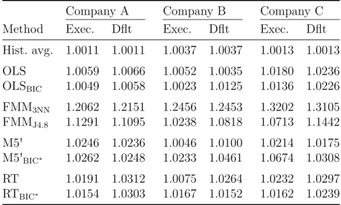
2.4 Results 27 For a better interpretation of the results, we also show the results of the his- torical average and two simple OLS regression models as benchmarks. We use identical explanatory variables for OLS regression as for the M5' algorithm and RT before applying the variable selection procedure. Similar to M5' and RT, we further apply a backward elimination to the OLS regression according to the BIC criterion in Equation (2.1).
We estimate the LGD at two different points in time: once at the execution of the contract and once at the time of default. Typically, more information is available at default, which should theoretically yield better predictions.
The in-sample and out-of-sample results are evaluated by calculating the Janus quotient introduced by Gadd and Wold (1964)
Janus =
v u u u u u t
1 n
n
P
i=1
(LGD
i−LGD
∗i,Oos)
21 m
m
P
i=1
(LGD
i−LGD
∗i,Is)
2 ,(2.7) with the in-sample estimation LGD
∗Isin the denominator and the out-of-sample estimation LGD
∗Oosin the numerator. Janus = 1 for equally large prediction errors for both estimations. A value close to 1 indicates a stable model and data structure.
At the end of the chapter, we also provide quality features of the identified finite mixture distributions and the error rates of classification for robustness reasons, and we interpret these results.
2.4.1 In-sample results
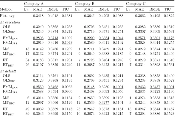
Beginning with the in-sample outcomes presented in Table 2.4, our models largely produce better estimations with the additional information available at default.
Our results clearly show the superiority of the FMMs for in-sample testing. The
MAE, RMSE, and TIC of the FMM
3NNare mostly far from their counterparts
Company A Company B Company C
Method Lv. MAE RMSE TIC Lv. MAE RMSE TIC Lv. MAE RMSE TIC Hist. avg. 0.3418 0.4018 0.1381 0.3646 0.4205 0.1988 0.3662 0.4195 0.1822 At execution
OLS 0.3240 0.3868 0.1268 0.2706 0.3451 0.1235 0.3282 0.3889 0.1519 OLSBIC 0.3246 0.3874 0.1272 0.2719 0.3471 0.1251 0.3307 0.3909 0.1537 FMM3NN 0.2806 0.3713 0.1099 0.2209 0.3354 0.1044 0.2571 0.3601 0.1176 FMMJ4.8 0.2919 0.3916 0.1043 0.2589 0.3911 0.1192 0.3028 0.3914 0.1255 M5' 13 0.3142 0.3786 0.1209 1 0.2711 0.3459 0.1241 2 0.3272 0.3874 0.1504 M5'BIC∗ 17 0.3132 0.3774 0.1201 9 0.2640 0.3388 0.1185 9 0.3148 0.3751 0.1400 RT 34 0.3183 0.3817 0.1231 7 0.2726 0.3464 0.1248 9 0.3279 0.3871 0.1510 RTBIC∗ 26 0.3197 0.3829 0.1240 11 0.2687 0.3423 0.1217 7 0.3314 0.3898 0.1531 At default
OLS 0.3114 0.3761 0.1191 0.2692 0.3435 0.1211 0.3238 0.3858 0.1490 OLSBIC 0.3123 0.3768 0.1195 0.2709 0.3451 0.1234 0.3238 0.3858 0.1527 FMM3NN 0.2550 0.3468 0.0955 0.2148 0.3280 0.1001 0.2432 0.3437 0.1091 FMMJ4.8 0.2588 0.3594 0.0900 0.2408 0.3693 0.1056 0.2835 0.3723 0.1190 M5' 6 0.3014 0.3680 0.1134 2 0.2650 0.3399 0.1193 1 0.3274 0.3883 0.1513 M5'BIC∗ 12 0.2997 0.3666 0.1126 12 0.2539 0.3277 0.1101 3 0.3244 0.3858 0.1490 RT 49 0.3032 0.3689 0.1143 25 0.2642 0.3373 0.1181 13 0.3247 0.3844 0.1487 RTBIC∗ 39 0.3046 0.3699 0.1150 10 0.2674 0.3422 0.1215 7 0.3294 0.3886 0.1523
Table 2.4: In-sample estimation errors at the execution and default of contracts by company. The best results are underlined for each company and type of error. Hist. avg.
is the historical average loss given default (LGD) used as estimation of the LGD. OLS represents the ordinary least squares regression, and FMM is the finite mixture model in combination with 3-nearest neighbors (3NN), or J4.8. OLS is also performed with the variable selection BIC algorithm and the M5' algorithm and the RT are performed with the variable selection BIC∗ algorithm. Lv. defines the number of leaves on the tree.
MAE is the mean absolute error defined in Equation (2.4) and RMSE is the root mean squared error defined in Equation (2.5). TIC is the Theil inequality coefficient defined in Equation (2.6). For MAE, RMSE, and TIC, lower outcomes are preferable.
![Figure 2.1: Density of the realized loss given default (LGD) by company. The realized LGD concentrates on the interval [ − 0.5, 1.5]](https://thumb-eu.123doks.com/thumbv2/1library_info/3757462.1510682/33.892.206.735.115.465/figure-density-realized-default-company-realized-concentrates-interval.webp)