Essays on Mechanism Design & Industrial Organization

Essays on

Mechanism Design &

Industrial Organization

Inauguraldissertation zur Erlangung des Doktorgrades der Wirtschafts- und Sozialwissenschaftlichen Fakult¨ at der

Universit¨ at zu K¨ oln

2017

vorgelegt von

Diplom–Volkswirt Andreas Pollak aus

Andernach am Rhein

Referent: Prof. Dr. Axel Ockenfels Korreferent: Prof. Dr. Oliver G¨urtler Datum der Promotion: 29.08.2017

Acknowledgments

During the last four years I strongly benefited from my coauthors, colleagues and friends who inspired, encouraged and supported me on many dimensions.

First and foremost, I want to thank my supervisor and coauthor Axel Ockenfels for his continuous guidance, encouraging feedback and for giving me the opportunity to do research at his chair.

I am also very grateful to my coauthors Felix Bierbrauer, Jos Jansen and D´esir´ee R¨uckert for the fruitful collaborations and inspiring discussions.

Furthermore, I would like to thank Oliver G¨urtler for co-refereeing this thesis and Marina Schr¨oder for chairing the defense board.

I gratefully acknowledge financial support provided by the German Research Foundation through the Leibniz program and through the DFG research unit “Design

& Behavior – Economic Engineering of Firms and Markets (FOR 1371)”. Further I acknowledge support from “The Excellence Center for Social and Economic Behavior at the University of Cologne (C-SEB)”.

I am also very thankful to my current and former colleagues for an enjoyable and cooperative working environment. In particular, I thank Kevin Breuer, Michael Cristescu, Christoph Feldhaus, Andrea Fix, Kiryl Khalmetski, David Kusterer, Felix Lamouroux, Susanne Ludewig-Greiner, Johannes Mans, Uta Schier, Margit Schmidt and Peter Werner. I always enjoyed working with you!

I also want to thank our current and former student research assistants Fabian Balmert, Andreas Gl¨ucker, Zena Kießner, Franziska Neder, Miriam Sobotta and Wolfram Uerlich. Particularly, I am indebted to Markus Baumann, Paul Beckmann, Max R. P. Grossmann, Lea Lamouroux, Yero Ndiaye, Frank Undorf and Johannes Wahlig for their valuable support and friendship.

Last but not least, I am deeply grateful to my parents, Norbert and Ilse, my brother Christian, my grandmother Christel as well as my girlfriend Andrea, her mother Ulrike and all my friends. It is good to have you!

Contents

1 Introduction 1

2 Do Price-Matching Guarantees with Markups Facilitate Tacit

Collusion? Theory and Experiment 5

2.1 Introduction . . . 6

2.2 Previous literature . . . 7

2.3 Theory . . . 10

2.3.1 Framework . . . 10

2.3.2 Market demand in equilibrium . . . 11

2.3.3 Equilibrium pricing without guarantees - The competitive benchmark case . . . 13

2.3.4 Equilibrium pricing with guarantees . . . 16

2.3.5 Summary of results . . . 21

2.4 Experiment . . . 22

2.4.1 Design and hypotheses . . . 22

2.4.2 Results . . . 25

2.5 Conclusion . . . 29

2.A References . . . 30

2.B Proofs . . . 33

2.C English Instructions (translated) . . . 47

2.D German Instructions (original) . . . 54

3 Strategic Disclosure of Demand Information by Duopolists: Theory and Experiment 60 3.1 Introduction . . . 61

3.2 The model . . . 64

3.3 Theoretical analysis . . . 65

3.3.1 Equilibrium outputs . . . 65

3.3.2 Equilibrium disclosure strategies . . . 67

3.3.3 Bertrand competition . . . 71

3.3.4 Hypotheses . . . 72

3.4 Experimental analysis . . . 75

3.4.1 Design . . . 75

3.4.2 Results . . . 79

3.5 Conclusion . . . 88

3.A References . . . 90

3.B Mathematical appendix . . . 93

3.C Table of test results & Stability of disclosure behavior . . . 107

3.D English Instructions (translated) . . . 110

3.E German Instructions (original) . . . 142

4 Robust Mechanism Design and Social Preferences 151 4.1 Introduction . . . 152

4.2 Related literature . . . 158

4.3 Mechanism design with and without social preferences . . . 160

4.3.1 The bilateral trade problem . . . 162

4.3.2 Optimal mechanism design under selfish preferences . . . 165

4.3.3 An observation on models of social preferences . . . 169

4.3.4 Social-preference-robust mechanisms . . . 172

4.3.5 Optimal robust and externality-free mechanism design . . . . 174

4.4 A laboratory experiment . . . 178

4.5 Which mechanism is more profitable? . . . 181

4.6 Redistributive income taxation . . . 183

4.7 Concluding remarks . . . 191

4.A References . . . 194

4.B Proofs . . . 199

4.C Other models of social preferences . . . 203

4.D Externality-freeness as a necessary condition. . . 206

4.E Supplementary material . . . 210

4.F English Instructions (translated) . . . 214

4.G German Instructions (original) . . . 219

5 Curriculum Vitae 223

Chapter 1

Introduction

Allocation rules, information sharing requirements or precommitments of firms to specific actions can strongly influence the outcome of a market. The understanding of how these features affect incentives of players in a given context is hence essential for market designers, antitrust authorities and legislators. In the following three chapters of this dissertation these effects are analyzed. Methodologically, all chap- ters have in common that they first develop and discuss a game theoretic model, which is then used for the derivation of hypotheses that are tested in a laboratory experiment. Each chapter thereby connects to and extends previous findings in industrial organization, experimental economics or mechanism design.

A key difference between the chapters lies in the level of abstraction. Chapter 2 analyzes specific price commitments of firms in a well-defined market environment.

Chapter 3 looks more generally at the incentives of firms for sharing information in environments which differ in the degree of information asymmetry and the type of competition. Finally, the last chapter examines how institutions in general can be designed to lead to a desired outcome, even if players have social preferences which are unknown to the market designer.

Chapter 2 is motivated by a new low-price guarantee which was recently intro- duced in the German gasoline market by Shell.¹ The guarantee promises to regis- tered customers of Shell that its effective gasoline price never exceeds the current price of any regional competitor by more than 2 Cents. In addition, this guarantee does not need to be explicitly claimed by participating customers, but is imple- mented automatically since Shell checks every purchase with a complete and real- time dataset from the German antitrust authority on whether the conditions of its guarantee are met. This chapter investigates, how this new type of price guarantee in general influences competition and, in particular, whether it can induce collusive high prices.

To this end, we analyze the guarantee in a sequential Hotelling duopoly model with two symmetric competitors which are located at the opposite ends of a road and compete in prices for a homogeneous good. We find that whenever at least the price-leader, i.e. the first moving firm, provides a guarantee with a sufficiently low markup, the equilibrium price level in the market is on average at the monopoly price

1Chapter 2 is written without coauthors. Despite this, the termswe orus instead of I are used throughout the chapter for consistency with the following chapters.

level. The data from a laboratory experiment supports this theoretical prediction.

Here, we find that in the treatment where the first moving firm has a guarantee with a low markup, prices of both firms are significantly higher in comparison with the treatments where the markup is high, or no price guarantee is in place.

The findings contribute to the previous theoretical and experimental literature on perfect price-matching guarantees and emphasize that this new type of price guarantee should be carefully reviewed by regulators and antitrust authorities.

Chapter 3 is joint work with Jos Jansen. It is motivated by a conflict between accounting rules and antitrust policies.² In particular, antitrust authorities are typ- ically skeptic about information sharing among competitors because this might lead to price coordination, while accounting rules often force firms to publicly disclose information in order to protect investors. This chapter studies strategic incentives for the disclosure of private information by firms about common market character- istics, like input costs or the demand level, and the corresponding consequences for the market outcome.

For the analysis, we use a duopoly model with incomplete information on a common demand intercept. This intercept can be either high or low and is drawn according to some distribution. Each duopolist can learn the intercept with a pre- defined probability. If they are successful in learning, they can voluntarily share this information with their competitor before competing with each other in a product market. Within this framework, we vary the demand distribution, the chances of learning the intercept and whether the competition is in prices or quantities.

We find that, independently on the variation of the model, firms selectively disclose information in order to gain a strategic advantage. By doing this, they manage their competitor’s belief about the demand intercept as well as about their own conduct. Hereby, they manipulate their competitor’s conduct in the product market in a way favorable for them. However, what kind of information they disclose and how strong the disclosure affects the market outcome depends on the information asymmetries among firms and the type of competition. With Cournot competition, firms typically disclose low demand and conceal high demand. However, we also identify conditions under which one Cournot competitor follows this strategy and

2Both authors were equally involved in generating the general research ideas, the experimental design as well as the hypotheses and in writing the draft. The theoretical model was developed by Jos Jansen. Mathematical proofs were done by Jos Jansen. The experiment was programmed, planned and conducted by Andreas Pollak. Statistical analyses were carried out by Andreas Pollak.

— The chapter is a modified version of Jansen and Pollak (2015). The data collection for the homogenous goods Cournot treatments and parts of the empirical analysis regarding the first hypothesis was done in Pollak (2012). The current version of the chapter was submitted to the

“International Journal of Industrial Organization” where it received a Revise & Resubmit.

the other chooses the reverse strategy. Moreover, the reverse disclosure strategy is always chosen in Bertrand competition, irrespective of the demand distribution and the degree of information asymmetry.

The chapter connects to previous theoretical and experimental studies on infor- mation disclosure. In particular, it is related to a paper by Ackert et al. (2000) who find evidence for selective disclosure in a model where only one firm has the ability to obtain and share information. We replicate and extend their findings by considering bilateral disclosure decisions, Bertrand competition, and information asymmetries between firms. We show that the previous finding of selective disclosure is robust to various kinds of market environments. In addition, we provide a tool to examine the resulting effect of disclosure on the market outcome.

In summary, our results help to evaluate the effects of economic policies regu- lating information disclosure by firms, such as competition policies or accounting rules.

Chapter 4 is joint work with Felix Bierbrauer, Axel Ockenfels and D´esir´ee R¨uck- ert.³ Standard mechanism design literature takes selfish preferences of players for granted. Consequently, the mechanisms proposed by this literature might system- ically fail when players are motivated by social preferences. In this chapter, we compare standard mechanisms with social-preference-robust mechanisms by study- ing two classical challenges of mechanism design, the bilateral trade problem and the problem of optimal income taxation.

For the bilateral trade problem, we first characterize a standard optimal and seller surplus maximizing mechanism, where the “buyer” and the “seller” are expected to truthfully report their type. We test this mechanism in a laboratory experiment and find that a non-negligible fraction of high valuation buyers understate their valua- tion. This finding contradicts to the underlying assumption of selfish preferences in classical mechanism design but is consistent with models of social preferences such as Fehr and Schmidt (1999) and Falk and Fischbacher (2006). We then characterize a mechanism which is externality-free, i.e. where each player’s equilibrium payoff does not depend on the other player’s type, and is thus social-preference-robust.

Testing this mechanism in the laboratory, we find that there are no longer devia- tions from truth-telling. Hence, the social-preference-robust mechanism is able to

3The research question and the experimental design were developed by Felix Bierbrauer and Axel Ockenfels, with comments from Andreas Pollak and Desiree R¨uckert. The theoretical analysis was done by Felix Bierbrauer and Desiree R¨uckert. The experiment was planned, programmed and conducted by Andreas Pollak. The statistical analyses were carried out by Andreas Pollak. All authors contributed equally to writing the paper. The current version of the paper is forthcoming in the “Journal of Public Economics”.

induce the desired outcome. However, in theory under the standard assumption of selfish preferences, this social-preference-robust mechanism is inferior in terms of performance relative to the standard mechanism, because the implementation of externality-freeness comes with a cost. Due to this cost, the standard mechanism outperformed the social-preference-robust mechanism in the experiment as the num- ber of deviations in the former was too small to compensate for that cost. Based on this observation, we engineered a hybrid mechanism by implementing externality- freeness only for the cases where a deviation from truthful behavior was observed, and tested it in the laboratory. In this experiment, the hybrid mechanism outper- formed the standard mechanism in terms of both truth-telling and performance.

For the problem of optimal income taxation, we compare a mechanism proposed by Piketty (1993), which is optimal in the classical sense, with a mechanism of Mir- rlees (1971) which is externality-free. In an additional experiment, we find that the (globally) externality-free Mirrleesian mechanism outperforms the standard optimal (but not social-preference-robust) mechanism by Piketty in terms of both truthful reporting and welfare.

Thus, Chapter 4 shows theoretically and experimentally that classic mechanisms can fail in generating a desired outcome, whereas externality-free mechanisms can preclude players from untruthful reporting. Whether a classic or a social-preference- robust mechanism is superior in terms of performance depends on the extent of deviations of players from truth-telling in the former. If the market designer knows where deviations can be expected, externality-freeness can be implemented locally and at a lower cost.

Chapter 2

Do Price-Matching Guarantees with Markups Facilitate Tacit Collusion?

Theory and Experiment ^∗

Andreas Pollak University of Cologne

Abstract

This paper studies how competitive prices are affected by price-matching guarantees allowing for markups on the lowest competing price. This new type of low-price guarantee was recently introduced in the German retail gasoline market. Using a sequential Hotelling model, we show that such guarantees, similar to perfect price- matching guarantees, can induce collusive prices. In particular, this occurs if the first mover provides a price guarantee with a markup which is below a threshold value. In these cases, prices are on average set at the monopoly level. A laboratory experiment supports the theoretical predictions.

Keywords: price-matching guarantee, tacit collusion, Hotelling, spatial competi- tion, sequential pricing, laboratory experiment

JEL Codes: C92, D21, D22, D43, L11, L13, L41

∗The research project was funded by The Excellence Center for Social and Economic Behavior at the University of Cologne via aJunior Start-up Grant of e3,000, which is gratefully acknowl- edged. I also acknowledge support from theGerman Research Foundation, who fund theCologne Laboratory for Economic Researchwhere the experiment was conducted. I thank Axel Ockenfels, Oliver G¨urtler, Felix Bierbrauer and my colleagues at the chair for helpful advice. I also thank Alexander Rasch, Achim Wambach and all other participants of theLenzerheide Seminar on Com- petition Economics 2016 for valuable comments. Finally, special thanks go to Kiryl Khalmetski for careful proof reading and Yero Ndiaye, who did a great job in assisting conducting the laboratory experiment. Naturally, all errors are mine.

2.1 Introduction

Since summer 2015, Shell promotes a new kind of low-price guarantee for standard gasoline: a price-matching guarantee with a markup on the lowest competing price within the regional market. In order to benefit from this guarantee, Shell’s customers have to register once, which is free of charge. Hereafter, Shell automatically checks for any purchase whether the posted gasoline price exceeds the lowest competing price by more than 2 Cents per liter, and, if this is the case, reduces its selling price to the lowest price plus the markup of 2 Cents.¹

The introduction of the guarantee followed a change in the design of the gasoline retail market, implemented by the German antitrust authority in 2013. More pre- cisely, the Bundeskartellamt established a real-time database for standard gasoline and diesel, called theMarkttransparenzstelle f¨ur Kraftstoffe or market transparency unit, and forced almost all gasoline retailers to keep their prices in the database up to date.² The market transparency unit is accessible for anyone free of charge via var- ious websites or smart-phone apps. The purpose of its introduction was to increase competition in the German gasoline retail market, as this market was found to be prone to (tacit) price coordination.³ However, it also enabled Shell to introduce this kind of guarantee, by providing the data for its automatic price comparisons. This made the guarantee especially attractive to customers, because they do not incur any costs of invoking the guarantee.

The question arising from this motivating example is whether this new kind of low-price guarantee might have an anti-competitive effect. Previous theoretical, em- pirical and experimental literature suggests that perfect price-matching guarantees are anti-competitive if the costs of invoking the guarantee are low. In contrary, other forms of low-price guarantees, especially price-beating guarantees, can even be pro- competitive. In a nutshell, the anti-competitive effect of the perfect price-matching guarantees results from making it virtually impossible to effectively undercut a ri- val’s price. However, this argument does not apply if the guarantee comes with a markup, since effective undercutting within the markup is possible. To the authors best knowledge, no previous theoretical or experimental paper studied the effect of a price guarantee with a maximal markup on competing prices, except for a re- cent empirical study by Dewenter and Schwalbe (2015), who find evidence for an anti-competitive effect of Shell’s guarantee.

1For exact condition terms of the guarantee see Shell Deutschland Oil GmbH (2016).

2See Bundeskartellamt (2014, 2015) for details.

3See Bundeskartellamt (2011).

This paper intends to close this gap. First, it analyzes the effects of price- matching guarantees with non-negative markups on competition in a theoretical framework inspired by the motivating example. Second, the obtained theoretical predictions are tested in a laboratory experiment. Both, theoretical and experimen- tal results show that the guarantee with a non-negative markup can indeed induce price coordination and leads to (on average) monopoly prices in these cases.

The remainder of the paper is structured as follows. The second section provides a brief overview of previous theoretical, experimental and empirical literature on low-price guarantees. The third section theoretically analyzes the price guarantee with a markup in a sequential Hotelling framework with two symmetric firms com- peting in prices and producing homogeneous goods. The fourth section presents an experimental design which is used to test the main theoretical predictions. Finally, the last section summarizes and discusses the results.

2.2 Previous literature

The effects of low-price guarantees have been discussed extensively in the economics and law literature since the early 1980s.⁴

Salop (1986) was the first to intuitively point out that perfect price-matching guarantees potentially lead to inefficient and anti-competitive market outcomes.

The basic idea is that, when a firm faces a competitor with a perfect price-matching guarantee, its incentive to undercut the competitor’s price is dampened since hisre- bate mechanism effectively creates a penalty (Salop, 1986, p.16), as individual price cuts become mutual. Accordingly, whenever all firms offer price-matching in mar- kets with simultaneous price competition, new equilibria arise with prices above the competitive level. This was later formalized by Doyle (1988). A further study by Logan and Lutter (1989) shows that under certain conditions, it is sufficient for a collusive market outcome if at least one firm offers a perfect price-matching guar- antee. The authors endogenize the adoption of perfect price-matching guarantees in a model with asymmetric costs, differentiated goods and simultaneous price com- petition. They find that only the high-cost firm offering a guarantee can induce an anti-competitive market outcome. In particular, if cost asymmetries are small, it adopts the guarantee and hereby creates incentives for supra-competitive pricing, whereas under large asymmetries it does not offer price-matching.

Additional literature focuses on further potentially negative effects of price match- ing guarantees. Edlin and Emch (1999) study the role of market entry and find

4Hviid (2010) provides a detailed survey.

that in markets with perfect price-matching, new entrants are attracted by collusive profits and also adopt the given pricing strategy. Hence, these entries only create inefficiencies, due to their entry and fixed costs, without making prices more com- petitive. Furthermore, Corts (1996) and Chen et al. (2001) suggest that low-price guarantees can be a tool to facilitate price discrimination between informed and uninformed customers, as only the former can invoke the guarantee. Consequently, in most cases uninformed customers loose whereas informed customers gain.⁵

In line with the previous argumentations Hay (1982), Sargent (1993) and Edlin (1997) advocate in favor of legislative prohibition of low-price guarantees and advise anti-trust authorities to at least carefully monitor markets in which they are used.

Further theoretical literature points out restrictions of the previous arguments against low-price guarantees. Hviid and Schaffer (1999) introduce the term has- sle costs, which subsumes all non-pecuniary costs of invoking the guarantee. They show that whenever hassle costs exist, a perfect price-matching guarantee does not prevent a competitor from undercutting within the hassle costs, since customers would not enforce the guarantee in these cases. This reasoning implies that in the presence of hassle costs, price-matching guarantees do not give rise to collusive equi- libria in symmetric markets, while in asymmetric markets the potential for collusive outcomes is limited.⁶ Moorthy and Winter (2006) show that in highly asymmetric markets with costly information, low-costs firms adopt price guarantees not to foster collusion, but rather as a signaling device. In these cases, under certain conditions low-price guarantees can increase welfare.

A different strand of literature studies price-beating guarantees, i.e. promises to strictly underbid the lowest competing price to a certain percentage or amount.

Hviid and Schaffer (1994) as well as Corts (1995) find that these guarantees do not lead to collusive market outcomes and in turn can be used to offset perfect price-matching guarantees. The reason is that price-beating guarantees reestablish the firms’ ability to unilaterally undercut prices, even if the competitors offer price- matching or beating. Intuitively, by posting a higher price, a firm offering a price- beating guarantee forces itself to effectively undercut the competitors’ prices, while at the same time the guarantees of the competitors are not activated. Kaplan (2000) criticizes these findings by pointing out that these results are restricted to price guarantees which pertain to posted prices, although admitting that these form of guarantees are empirically more relevant.

5Corts (1996) finds, for a special case where informed customers have the less elastic demand and firms can offer price-beating guarantees, that prices fall for both groups.

6Mao (2005) comes to a similar conclusion when focusing on the costs of returning of ex ante uninformed customers to stores that provide price-matching.

Empirical studies qualitatively confirm most of the theoretical results. For exam- ple, Hess and Gerstner (1991) study the price development of five supermarket chains in North Carolina in the mid 1980s. They find that after the first chain adopted a perfect price-matching guarantee for specific goods, the others followed suit by adopting similar guarantees. Consequently, prices of the goods included in the guar- antees rose significantly in comparison to those excluded, while the differences in the former prices almost vanished completely. Arbatskaya et al. (2004) study over 500 price guarantees by using data from newspaper advertisements. They find that 56 percent of the perfect price-matching guarantees and only about 10 percent of the price-beating guarantees led to pricing above the competitive level. In addition, they find that most of the latter referred to posted instead of effective prices. A further study by Arbatskaya et al. (2006) comes to a similar conclusion when re- viewing low-price guarantees in the retail tire market. Moorthy and Winter (2006) as well as Moorthy and Zhang (2006) find support for the usage of price-matching guarantees as signaling device by low-cost firms. A recent paper by Dewenter and Schwalbe (2015) studies the effect of low-price guarantees in the German gasoline market. With a difference-in-difference panel regression, controlling for exogenous effects and using data from the market transparency unit, they examine changes in pricing of two chains which recently started offering low-price guarantees. For the chain HEM, which are offering a non-automatic prefect price-matching guarantee, they do not find any significant price effect. The authors speculate, that this is a result of the relative high hassle costs customer faces for invoking the guarantee. For Shell’s hassle cost free price-matching guarantee with a markup, the authors find a significant price increase by Shell of 2.4–2.8 Cent per liter standard gasoline after the introduction of the guarantee.

Furthermore, experimental literature also supports most of the theoretical im- plications. Dugar (2007) and Mago and Pate (2009) consider perfect price-matching guarantees and focus on the resulting equilibrium selection in symmetric and asym- metric markets with homogeneous goods and simultaneous pricing. They find evi- dence for the selection of the most collusive equilibrium, as long as the asymmetries in costs are sufficiently small. In addition, Fatas and Manez (2007) and Fatas et al.

(2013) results support the prediction that perfect price-matching guarantees lead to a collusive outcome when symmetric firms compete simultaneously in a market with differentiated goods. Finally, Fatas et al. (2005) find no evidence that price-beating guarantees cause an anti-competitive market outcome.

2.3 Theory

2.3.1 Framework

The model is based on the Hotelling duopoly framework with linear transportation costs. There are two firms producing a homogeneous good, which are located at the opposite ends of a road and compete in prices (Hotelling, 1929).

Customers are uniformly distributed along the road, normalized to a mass of 1, and have a valuation of v > 0 for a unit of the good. They behave as price takers, since they are infinitely many. Customers have full transparency about prices and incur linear transportation costs of t > 0 times the distance to their dealer. The transportation costs are assumed to be moderate, i.e. t < ^v₃, which keeps the analysis simple and assures that the firms serve the entire road in equilibrium. All customers behave rationally and have a single unit demand. Thus, they buy at the best deal they can get whenever their net benefit is positive, otherwise they do not buy at all.

Firms do not face capacity constraints and incur neither fixed nor variable costs.

They are allowed to set any non-negative price, i.e. dumping is prohibited. Firm A is located at the left end of the road, at positionx_A= 0. The main new element of the model is that it provides a price-matching guarantee with an (exogenous) markup m≥ 0.⁷ That is, it guarantees to customers that it never exceeds the competitor’s price by more thanm.⁸ Firm B is located at the right end of the road, i.e. atx_B = 1, and offers no price guarantee. Restricting to only Firm A offering a price guarantee is sufficient to show the collusive effect of the price guarantee. In Appendix 2.B we prove that any version of the model where Firm B additionally has an arbitrary price guarantee with a non-negative markup leads to identical prices in equilibrium, compared to the game with only Firm A offering such a guarantee.

The timing of the game is as follows. In the first stage, Firm A chooses its posted price p^p_A (i.e. its initially announced price). After observing p^p_A, Firm B chooses its price p_B in the second stage. Based on these posted prices the effective price of Firm A, denoted as p_A, results by applying the guarantee, i.e.

pA:= min{p^p_A, pB+m} with m ∈[0, t[. (2.1)

7A markup smaller than zero would be an exotic form of a price-beating guarantee, which is activated if the competitors price is not sufficiently higher than the price of the guarantee issuing firm. For a discussion of price-beating guarantees see the previous literature section and the references therein.

8For simplification, the analysis is restricted to cases where m < t, since otherwise the market share would be zero for Firm A whenever the price guarantee is active.

The effective price of Firm B always equals its posted price. Once the effective prices are determined, customers make their purchasing decisions, and the game ends.

The game is solved by backward induction, i.e. the solution concept is a sub-game perfect Nash equilibrium.

2.3.2 Market demand in equilibrium

Now, we derive the market demand function of Firmi. The location of the customer who is indifferent between purchasing at Firm A or Firm B is denoted by ˜x^AB (i.e. ˜x^AB ∈ [0,1] is the share of customers located to the left of this customer on the road). If this customer has a non-negative net benefit from consumption, his position determines market shares, since all customers to the left of him will buy at Firm A whereas all customers to the right of him will find it more profitable to buy at Firm B.

In general, a customer located at positionxgets a net benefit ofu^A_x from buying at Firm A, which equals his valuation minus the price and the incurred transportation costs:

u^A_x =v−p_A−x·t. (2.2)

The same customer receives a net benefit of u^B_x if he instead buys at Firm B:

u^B_x =v−p_B−(1−x)·t. (2.3) Consequently, the location of the customer who is indifferent between Firm A and Firm B is

˜

x^AB = 1

2+ p_B−p_A 2t .

This position is interior (i.e., between 0 and 1) if and only if

p_A−t < p_B < p_A+t. (2.4) Naturally, being indifferent between buying at Firm A and Firm B does not neces- sarily assure that the customer is willing to buy at all. This is only the case if his net benefit of purchasing is non-negative, i.e. u^A_x˜AB =u^B_x˜AB ≥0. This is equivalent to:

p_B ≤2v−t−p_A. (2.5)

Next, we consider four possible cases depending on the location and preferences of the indifferent customer.

Case 1: Condition (2.5) is not satisfied, while the indifferent customer does not exist along the road. The non-existence of the indifferent customer implies that condition (2.4) does not hold, i.e. the price difference between the firms exceeds the highest possible transportation cost. Then, all customers on the road prefer the firm with the lower price over the other firm (whose demand is then 0 anyway). The former firm hence faces a monopolistic demand function:

D_M(p_i) =















1 if p_i ≤v −t, v−pi

t if v−t < p_i < v,

0 else.

(2.6)

Case 2: Condition (2.5) is not satisfied, while the indifferent customer exists along the road. In this case, there exists a range of customers along the road who do not buy from any of the firms. Then, firms do not effectively compete with each other, since the price of one firm does not affect the demand of the other, and hence again face a monopolistic demand function given by (2.6), except that the first segment withD_M(p_i) = 1 does not exist in this case.

Case 3: Condition (2.5) is satisfied, while the indifferent customer does not exist along the road. Then, as in Case 1, the firm with a higher price has a demand of zero, while the firm with a lower price faces monopolistic demand. However, one can show that under considered conditions it always holds for the latter firm that p_i ≤v−t, which by (2.6) implies that it demand is 1.

Case 4: Condition (2.5) is satisfied, while the indifferent customer exists along the road. In this case, the indifferent customer prefers to buy the good over not buying.

Hence, Firm A (B) faces competitive demand given by the fraction of customers positioned to the left (right) from the indifferent customer. That is, the market demand for Firm i∈ {A, B}, denoted as D_i, is a function of the effective prices p_i and p_−i:

D_i(p_i, p_−i) = 1

2 +p_−i−p_i

2t . (2.7)

Finally, note that a firm gets a demand of 1 if and only if the following condition is satisfied:

Lemma 1. Firmireceives the whole demand if and only ifp_i ≤v−tandp_i < p−i−t.

Proof. A given firm receives the whole demand if and only if the following two incentive constraints for the customers are satisfied: 1) all customers prefer buying from this firm over not buying; 2) all customers prefer buying from this firm over buying from the other firm. Given (2.2) and (2.3), these conditions are equivalent

to the conditions stated in the lemma.

Thus, summing up all four cases and taking Lemma 1 into account, the market demand for Firmi∈ {A, B} is:

D_i(p_i, p−i) =



























1 ifp_i ≤v−t ∧ p_i < p−i−t , 1

2 +p−i−p_i

2t ifp_i ≤2v−t−p−i ∧ p_i ∈[p−i−t, p−i+t], v−p_i

t ifp_i >2v−t−p−i ∧ p_i ∈]v−t, v[,

0 else.

(2.8)

2.3.3 Equilibrium pricing without guarantees - The competitive benchmark case

To begin, we relax the assumption that Firm A offers a price guarantee and look what happens in the competitive benchmark case, i.e. p^p_A=p_A.⁹ In the next section, we will then consider the model with Firm A having a price-matching guarantee with a non-negative markup, as described above.

In stage 2, Firm B knows p^p_A and maximizes π_B by choosing the optimal p_B. Since Firm A’s posted price is also its effective price and given (2.8), we get the following piecewise defined profit function:

π^{N o P G}_B (pB, p^p_A)=































pB ifpB ≤v−t ∧ pB < p^p_A−t , p_B·

1

2 +p^p_A−p_B 2t

ifp_B <2v−t−p^p_A ∧ p_B ∈[p^p_A−t, p^p_A+t], p_B·

v−pB

t

ifp_B ≥2v −t−p^p_A ∧ p_B∈]v−t, v[,

0 else.

(2.9)

9This is technically equivalent to offering a guarantee with an infinitely high markup on the competitor’s price, which therefore cannot be activated.

This implies the following result:

Proposition 1. Firm B’s reaction function, when Firm A does not provide a price guarantee, is given by:

R^{N o P G}_B (p^p_A) =



















v−t if p^p_A > v, p^p_A−t if 3t ≤p^p_A ≤v,

p^p_A+t

2 if p^p_A <3t.

Proof. See Appendix 2.B.

Thus, Firm B’s best response depends on p^p_A being in one of three different cases.

Now, we discuss the intuition for B’s best response in each of these cases.

Case 1 – Firm A posts a prohibitively high price, i.e. p^p_A> v. In this case, Firm B is de facto a monopolist. Since the transportation costs are moderate, a monopolist wants to serve the entire road and sets a price ofv−t.

Case 2 – Firm A posts a price between3tandv. In this interval,p^p_Ais not prohibitive, but high enough to make it profitable for Firm B to serve the full market on its own.

Thus, Firm B undercuts Firm A’s price just to the extent of the transportation costs.

Case 3 – Firm A posts a price between 0 and 3t. For this interval of p^p_A, it is not optimal, even in some cases not possible, for Firm B to serve the entire road. Hence, Firm B shares the market with Firm A. The price p_B = ¹₂(p^p_A+t) solves Firm B’s trade-off between gaining a higher market share and charging a higher price.

In the first stage, Firm A anticipates Firm B’s reaction function given by Propo- sition 1 and hence faces the following maximization problem:

argmax

p^p_A

π_A^{N o P G}(p^p_A)|R^{N o P G}_B =











0 if p^p_A≥3t,

p^p_A· 1

2 +t−p^p_A 4t

if p^p_A<3t

(2.10)

Ifp^p_Ais at least 3t, Firm B, according to Proposition 1, undercuts Firm A’s price at least byt. In these cases, the demand of Firm A will be zero, as even the closest customer atx= 0 would prefer to buy from Firm B.

If p^p_A is smaller than 3t, Firm B undercuts, if at all, to a lesser extent than t by setting p_B = ^p

p A+t

2 . In these cases, all conditions of the second case of the demand function in (2.8) are fulfilled: First,

p^p_A−p_B = p^p_A−t 2 < t, p_B−p^p_A = t−p^p_A

2 >−t, where the inequalities follow from p^p_A <3t. Second,

pB = p^p_A+t

2 ≤ 2v−t−p^p_A

⇔ p^p_A ≤ 4 3v−t,

which holds forp^p_A<3t because t≤ ^v₃. Thus, by (2.8), wheneverp^p_A is smaller than 3t the demand for Firm A is

1

2+ p_B−p^p_A 2t = 1

2+

1

2p^p_A+¹₂t−p^p_A

2t = 1

2+ t−p^p_A 4t ,

which implies the above profit maximization problem of Firm A. That is, if Firm A posts a price higher than 3t, Firm B will serve the market on its own and conse- quently A’s profits are zero, whereas for lower prices Firm A has to share the market with Firm B and the profits are equal to its market share multiplied by its charged price.

Solving the maximization problem of Firm A gives the optimal price of p^p_A = ³₂t.

Using Firm B’s reaction function and the demand function in (2.8), we obtain the equilibrium characterization of the competitive benchmark case in which Firm A does not provide a price guarantee:

p^p_A= 3

2t, p_B = 5

4t, D_A= 3

8, D_B = 5

8, π_A= 18

32t, π_B = 25 32t.

Note that Firm B is better off than Firm A in equilibrium, which results from the sequential structure of the game. Since prices are strategic complements, Firm B has a second mover advantage. It can profitably undercut Firm A’s price and hereby gain a higher market share as well as higher profits in equilibrium.

2.3.4 Equilibrium pricing with guarantees

In this subsection we assume that Firm A provides a guarantee with a non-negative markup on the competitor’s price.¹⁰ This includes, ifm is zero, also a perfect price- matching guarantee.

In the second stage Firm B maximizes its profit function

π_B^{P G}(p_B, p_A(p^p_A, p_B)) =







π_B^{N o P G}(p_B, p^p_A) if p_B ≥p^p_A−m , π_B^{P G−Active}(pB, pB+m) else.

That is, only if it undercuts the price of Firm A by no more than m, Firm A’s guarantee will not be activated and profits are defined byπ^{N o P G}_B . For any lowerp_B, the guarantee will be activated and the profits of Firm B are defined by (given the demand function (2.8)):

π_B^{P G−Active}(p_B, p_B+m) =





















 p_B·

1 2 +m

2t

if p_B ≤v− t+m 2 , p_B·

v−p_B t

if v− t+m

2 < p_B < v,

0 else.

(2.11)

Whenever Firm A’s price guarantee is active, the effective price difference between p_A and p_B equals the markup, independently of p_B. Consequently, the position of the customer being indifferent between buying at Firm A or B exists along the road, as the price difference m is by assumption smaller than t (see condition 2.4).

Hence, by the demand function in (2.8), whenever this customer finds it profitable to purchase a good, i.e. if condition (2.5) holds (which is then equivalent to p_B ≤ v− ^t+m₂ ), the market demands are fixed to D_A = ¹₂ − ^m_2t and D_B = ¹₂ + ^m_2t. This is plausible, as customers balance the trade-off between better (effective) prices and higher transportation costs. However, if p_B exceeds v − ^t+m₂ (i.e. the indifferent customer prefers not to buy), the demand is calculated with the demand function of a monopolist, stated in (2.6). Thus, forp_B ≤v−^t+m₂ profits are linearly increasing in p_B, whereas for higher prices profits are decreasing, so that the profits are maximized atpB =v− ^t+m₂ .

10As proven in Appendix 2.B, prices in equilibrium are identical if additionally Firm B provides a price-matching guarantee with a non-negative markup.

The following proposition derives the reaction function of Firm B maximizingπ_B^{P G}: Proposition 2. Firm B’s reaction function, when Firm A provides a price guarantee with a markup m on the competitor’s price, is given by:

R^{P G}_B (p^p_A) =



















v −t+m

2 if p^p_A> v− ^t−m₂ ,

p^p_A−m if t+ 2m < p^p_A≤v− ^t−m₂ , p^p_A+t

2 if p^p_A≤t+ 2m.

(2.12)

Proof. See Appendix 2.B.

Thus, Firm B’s reaction is dependent on p^p_A being in a specific interval. In the following paragraphs the intuition for the optimal choice of p_B is briefly discussed with the help of a graphical illustration for each of the three intervals.

p_B π^{P G}_B

ν−^t+m

2

ν

Figure 2.1: π^{P G}_B if p^p_A > v− ^t−m₂

Figure 2.1 depicts the profit function of Firm B for p^p_A > v − ^t−m₂ . Whenever p_B is below v − ^t+m₂ Firm A’s price guarantee is active while the market is fully covered. Hence, by (2.8), Firm B’s market demand is D_B = ¹₂ + ^m_2t, and thus constant. Therefore, profits are linearly increasing in this interval. For any higher p_B, condition (2.5) is violated, and thus, independently of whetherp_B might activate Firm A’s guarantee or not, Firm B faces monopolistic demand. Since the monopolist prefers to serve the entire road, Firm B’s profits are monotonically decreasing in this segment. Consequently, it is optimal to setp_B =v−^t+m₂ for anyp^p_A> v−^t−m₂ , since any higherp_B would lead to an unprofitable loss in market share and any lower price would trigger a harmful automatic reduction of Firm A’s price. The latter precludes Firm B from gaining any higher market demand.

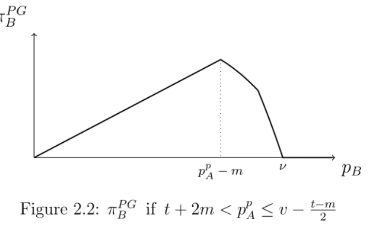
Figure 2.2 illustrates Firm B’s profits for posted prices in the interval [t + 2m, v−^t−m₂ ]. Analogously to the reasoning above, due to the price guarantee, it can not

p_B π_B^{P G}

p^p_A−m ν

Figure 2.2: π^{P G}_B if t+ 2m < p^p_A≤v− ^t−m₂

be optimal to setp_B< p^p_A−m, since this would result in decreased profits for both firms while leaving market shares unaffected. For any higherp_B, Firm B’s trade-off between charging at a higher price and gaining a higher demand is in favor of the demand, independently of whether p_B would violate condition (2.5) or not. As a resultπ_B^{P G} is decreasing in this segment. In summary,p^p_A is still sufficiently high so that Firm B has an incentive to undercut Firm A’s price just to the extent of the markup.

Figure 2.3 finally refers to the states where Firm A posted a price lower or equal 2m+t. Here, the posted price of Firm A is so low, that Firm B would not want to undercut it by more thanm, even if it could effectively do so. Thus, the optimal reaction for these posted prices is, similar to the competitive benchmark case, to set p_B = ^p

p A+t

2 .

p_B π_B^{P G}

p^p_A−m (p^p_A+t)/2 p^p_A+t

Figure 2.3: π^{P G}_B if p^p_A ≤t+ 2m

In summary, Firm B ensures in all cases that the market is fully covered and shared with Firm A, with a maximal market share of Firm B of ¹₂ +^m_2t.

Given Firm B’s reaction, given by Proposition 2, and the demand function in (2.8), Firm A faces the following maximization problem:

argmax

p^p_A

π_A(p^p_A)|R_B^{P G}=























v− t−m 2

· 1

2− m 2t

if p^p_A> v− ^t−m₂ , p^p_A·

1 2− m

2t

if t+ 2m < p^p_A≤v− ^t−m₂ , p^p_A·

1

2+ t−p^p_A 4t

if p^p_A≤t+ 2m.

(2.13) That is, for any posted price higher than t+ 2m, Firm A will serve a market demand of ¹₂−^m_2t, since Firm B will either undercut just to the extent of the markup or activate Firm A’s price guarantee (see Proposition 2). Moreover, its profits strictly increase in the interval [t+ 2m, v−^t−m₂ ] because its effective price will be the posted price as p_B will be set to just p^p_A−m. All posted prices higher than v − ^t−m₂ will result in an effective price of Firm A of v− ^t−m₂ , due to the activation of the price guarantee. Only for p^p_A ≤ t + 2m the maximization problem is identical to the problem of the competitive benchmark case.

The following proposition shows the optimal price of Firm A:

Proposition 3. In equilibrium, Firm A will set

p^p_A =







p^p_A≥v− t−m

2 if m < φ, 3

2t if m≥φ.

(2.14)

with φ= ¹₂√

4v² −9t²−v+t.

Proof. See Appendix 2.B.

According to Proposition 3 Firm A’s optimal price depends on the markup being above or below the critical threshold value φ. Whenever m < φ, Firm A can maximize its profits by setting any collusive arbitrary high price which is at least v− ^t−m₂ , since Firm B will then take care, that the market is jointly covered with the highest possible prices. For m ≥ φ Firm A’s optimal price coincides with the equilibrium price in the competitive benchmark case.

Figure 2.4 shows an example of Firm A’s profit function ifmis below the critical threshold value. Here, the local profit maximum in the competitive section, reached with the competitive price p^p_A = ³₂t in the example, is clearly below the maximum which can be achieved by setting a collusive price. This argument also holds if the

p^p_A π_A^{P G}

3

2t ν−^t−m₂

Figure 2.4: π_A^{P G} if m < φ

local maximum of the parabola is to the right of the competitive section, i.e. if

3

2t <2m+t.

Figure 2.5 portrays Firm A’s profit function whenm exceeds the critical thresh- old. Here, the profits from collusion are lower than the profits which can be achieved in the competitive segment. This results from the fact that the market division with collusion is increasingly disadvantageous for Firm A whenm gets larger.

p^p_A π_A^{P G}

3

2t ν−^t−m₂

Figure 2.5: π^{P G}_A if m≥φ

Finally, Proposition 2 and Proposition 3 together imply the following result, fully characterizing the effective prices in equilibrium.

Proposition 4. If Firm A offers a price guarantee with a non-negative markup of (a) m < φ, the effective price of Firm A is v − ^t−m₂ and the effective price of Firm B is v− ^t+m₂ , and hence prices equal on average the monopoly price of v− ^t₂. (b) m ≥φ, the effective price of Firm A is ³₂t, and the effective price of Firm B is ⁵₄t, and hence prices are the same as in the competitive benchmark case where no firm provides a guarantee.

Proof. See Appendix 2.B.

The intuition for Proposition 4 is simply that Firm A’s market share is decreasing in the size of the markup. Hence, if m exceeds φ, Firm A’s profit from setting a collusive price would be too small, so that it prefers to post the competitive price.

In contrast, ifm is below φ, the guarantee induces a collusive outcome.

2.3.5 Summary of results

Table 2.1 summarizes the results and compares equilibrium market outcomes across different kinds of competition.

It shows that whenever Firm A offers perfect price-matching, the market outcome is identical to a case where both firms are owned by a monopolist. This type of price guarantee is most attractive for Firm A, because it neutralizes the second mover advantage of Firm B, i.e. both firms share the monopoly profit ofv− ₂^t equally.

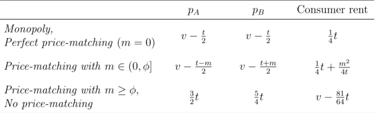
Table 2.1: Equilibrium Prices and Consumer Rent

p_A p_B Consumer rent

Monopoly,

v− ₂^t v− ₂^{t 1}₄t

Perfect price-matching (m= 0)

Price-matching with m∈(0, φ] v−^t−m₂ v−^t+m₂ ¹

4t+ ^m_4t² Price-matching with m≥φ, ₃

2t ⁵₄t v− ⁸¹₆₄t

No price-matching

According to Proposition 4, whenever Firm A is offering a price guarantee with a positive small markup, the average price level of both firms is still the monopoly price. However, due to the unequal market division, the profit of Firm A decreases when the markup gets bigger, whereas the profits of Firm B increase. The consumer rent in this case is slightly higher in comparison with perfect price-matching, as cus- tomers close to Firm B benefit from its lower prices and their gains overcompensate the losses of customers close to Firm A.

If Firm A offers a price guarantee with a high markup, the guarantee will be virtually ignored. Both firms set prices as in the competitive benchmark case, and accordingly rents and profits are unaffected by the guarantee.

2.4 Experiment

We conducted a laboratory experiment using the model-framework discussed in the previous section. We aim to investigate the collusive effects of guarantees with different maximum markups on the competitor’s price.

Background information. All treatments were programmed with the software z-Tree (Fischbacher, 2007) and all sessions were conducted in theCologne Laboratory for Economic Research at the University of Cologne in August 2016. Participants were randomly recruited from a sample of 1,500 students, enrolled in business ad- ministration or economics, via email with the Online Recruitment System ORSEE (Greiner, 2015). We conducted in total six sessions with 30 participants each. Each subject was only allowed to participate in one session. The share of males and fe- males, 53.3% and 46.7% respectively, was almost equal. The average age was 24.7 years. Payments to subjects consisted of a 4 Euro lump-sum payment for showing up, another 4 Euro for completing a short questionnaire and additional money which could be earned in every period, based on achieved profits. The currency used was Experimental Currency Units (ECU), which was converted to Euro at the end of the experiment at an exchange rate of 1 EUR per 14,000 ECU. Average individual payments including the lump-sum payments were 13.56 Euro. Each session took about one hour.

2.4.1 Design and hypotheses

The lab experiment was designed to test the extend of tacit collusion in the presence of guarantees. Three treatments were conducted: A baseline treatment without a price guarantee, a treatment with a markup below and a treatment with a markup above the threshold value φ, which determines whether a guarantee is expected to lead to collusive prices or not. In each treatment subjects were in role of either Firm A or Firm B and faced a computerized equilibrium demand function.

Besides the markup, all parameters were kept constant across treatments. The valuation of customers for a good was set to v = 200 and the transportation costs were set to t = 35. Given these parameters, the threshold value φ predicts that a price guarantee with a markup below 27.99 results in collusive prices, whereas guarantees with higher markups are expected to result in competitive prices. Addi- tionally, potential customers along the road were set to a mass of 100 instead of 1 in the previous section. This does not qualitatively change theoretical predictions, but scales up demand and profits and thus makes the experiment less artificial and easier

to explain in the instructions. In order to gain sufficient statistical power for the analysis, all treatments consisted of two sessions with 30 participants each. Since we used a matching group size of six, this resulted in 10 independent observations for each role in every treatment.

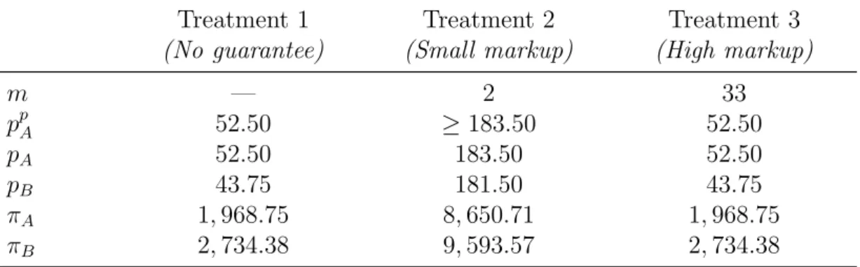
Table 2.2 summarizes the treatment design and states theoretical point predic- tions for posted as well as effective prices, and the corresponding equilibrium profits.

Table 2.2: Treatment Design and Point Predictions

Treatment 1 Treatment 2 Treatment 3

(No guarantee) (Small markup) (High markup)

m — 2 33

p^p_A 52.50 ≥183.50 52.50

p_A 52.50 183.50 52.50

pB 43.75 181.50 43.75

π_A 1,968.75 8,650.71 1,968.75

π_B 2,734.38 9,593.57 2,734.38

All values are stated in ECU.

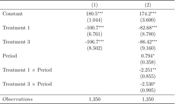
In Treatment 1 (T1) Firm A has no price guarantee. This treatment serves as the competitive benchmark. In equilibrium Firm A sets a price of 52.50. Firm B, due to its second mover advantage undercuts this by setting a price of 43.75. Consequently, Firm A’s price exceeds Firm B’s price by 20%, leading to a market coverage of 37.5%

for Firm A compared to 62.5% for Firm B. Due to the higher market share, Firm B gets a profit of 2,734.38, which exceeds Firm A’s profit of 1,968.25 .

In Treatment 2 (T2) Firm A has a price guarantee with a markup of m = 2.

Since this markup is below the threshold value φ, it induces a collusive market outcome in theory. In any equilibrium of T2, Firm A posts the collusive price of 183.50 or higher. Firm B undercuts the posted price but only to the extent of m plus the amount by which Firm A’s price exceeds 183.50. Put differently, Firm B sets 181.50 in any equilibrium and thus assures that the effective price of Firm A is 183.50. Consequently, effective prices are close to another and equilibrium market shares and profits are only in slight favor of Firm B, which serves 52.86% of the market and earns 9,593.57 compared to 47.14% and 8,650.71 for Firm A.

In Treatment 3 (T3) Firm A has a price guarantee with a markup of m = 33.

Since the markup is higher than φ, theory predicts that the guarantee does not affect effective prices, market shares and profit levels compared to a setting where no guarantee is in place. Thus, chosen price levels in this treatment are expected to coincide with the price levels of T1.

Hypotheses. In summary, we get two hypotheses from the treatment compar- isons. First, we expect the price guarantee with the small markup in T2 to lead to a collusive market outcome. That is, we expect Firm A and Firm B to set higher prices in T2 compared to T1. Second, we do not expect the price guarantee with the high markup to have any effect on competition. Consequently, the prices of Firm A and Firm B in T3 are expected not to differ compared to T1 but to be lower than in T2.

Procedures within the experiment. All treatments consisted of an individual trial stage, followed by an interaction stage consisting of 15 periods of the sequential pricing game.

Prior to the start of the experiment, subjects were randomly allotted to computer terminals. Then they received identical written instructions, explaining general lab rules, all treatment specific information, including the equilibrium demand function as well as the matching procedure in the interaction stage.¹¹ Whenever subjects had questions, these were answered privately by referring to the relevant section in the instructions.

The trial stage, which lasted approximately five minutes, started roughly ten minutes after the instructions were distributed. This stage was not payoff rele- vant, did not involve any interaction between subjects and consisted of a simple scenario-calculator which used continuous posted prices as inputs and showed re- sulting effective prices, market shares and profit levels as outputs. This calculator was identical for all subjects within a treatment, independently of the role a subject was assigned to in the subsequent interaction stage, where it was also accessible.

The purpose for providing the calculator was to allow subjects to deal with complex demand and profit calculations. By using a calculator with empty default values, it could be avoided to set anchoring points in contrast to providing payoff tables or examples, which inevitably put focus on certain price combinations. The scenario calculator could be used for any continuous price combination between 0 and 200.¹² Finally, subjects proceeded to the interaction stage, consisting of 15 identical periods of the sequential pricing game. Each subject was assigned to a specific role, either Firm A or Firm B, and a matching group consisting of 6 subjects. These

11The instruction in English language can be found in Appendix 2.C. The original German instructions are available upon request.

12Imposing an upper bound for posted prices was necessary, due to a technical reason: Subjects entered prices via a slider bar, which requires a lower and an upper bound. Thus, we have chosen to set the upper bound to the prohibitive price level of 200, since all posted prices higher than 200 are at least weakly dominated. Thus, this restriction does not affect the equilibrium point predictions stated in Table 2.2.