The Unreasonable Fairness of Maximum Nash Welfare

The Unreasonable Fairness of Maximum Nash Welfare

IOANNIS CARAGIANNIS , University of Patras

DAVID KUROKAWA , Carnegie Mellon University

HERV ´ E MOULIN , University of Glasgow and Higher School of Economics, St Petersburg

ARIEL D. PROCACCIA , Carnegie Mellon University

NISARG SHAH , Carnegie Mellon University

JUNXING WANG , Carnegie Mellon University

The maximum Nash welfare (MNW) solution — which selects an allocation that maximizes the product of utilities — is known to provide outstanding fairness guarantees when allocating divisible goods. And while it seems to lose its luster when applied to indivisible goods, we show that, in fact, the MNW solution is unexpectedly, strikingly fair even in that setting. In particular, we prove that it selects allocations that are envy free up to one good — a compelling notion that is quite elusive when coupled with economic efficiency.

We also establish that the MNW solution provides a good approximation to another popular (yet possibly infeasible) fairness property, the maximin share guarantee, in theory and — even more so — in practice.

While finding the MNW solution is computationally hard, we develop a nontrivial implementation, and demonstrate that it scales well on real data. These results lead us to believe that MNW is the ultimate solution for allocating indivisible goods, and underlie its deployment on a popular fair division website.

CCS Concepts: •Theory of computation→ Algorithmic mechanism design; •Applied computing→

Economics;

Additional Key Words and Phrases: Fair division, Resource allocation, Nash welfare

1. INTRODUCTION

We are interested in the problem of fairly allocating indivisible goods, such as jewelry or artworks. But to better understand the context for our work, let us start with an easier problem: fairly allocating divisible goods. Specifically, let there be m homoge- neous divisible goods, and n players with linear valuations over these goods, that is, if player i receives an x

fraction of good g, her value is v

(x

) = P

g

x

v

(g), where v

(g) is her non-negative value for the (entire) good g alone.

The question, of course, is what fraction of each good to allocate to each player;

and it has an elegant answer, given more than four decades ago by Varian [1974].

Under his competitive equilibrium from equal incomes (CEEI) solution, all players are endowed with an equal budget, say $1 each. The equilibrium is an allocation coupled with (virtual) prices for the goods, such that each player buys her favorite bundle of

This work was supported in part by the National Science Foundation under grants IIS-1350598, CCF- 1215883, and CCF-1525932; by a Sloan Research Fellowship; by the COST Action IC1205 on “Computational Social Choice”; and by the Caratheodory research grant E.114 from the University of Patras.

Authors’ addresses: I. Caragiannis, University of Patras, Greece; email: caragian@ceid.upatras.gr; D.

Kurokawa, Carnegie Mellon University, USA; email: dkurokaw@cs.cmu.edu; H. Moulin, University of Glas- gow, UK, Higher School of Economics, St Petersburg, Russia; email: Herve.Moulin@glasgow.ac.uk; A. D. Pro- caccia, Carnegie Mellon University, USA; email: arielpro@cs.cmu.edu; N. Shah, Carnegie Mellon University, USA; email: nkshah@cs.cmu.edu; J. Wang, Carnegie Mellon University, USA; email: junxingw@cs.cmu.edu.

Permission to make digital or hard copies of all or part of this work for personal or classroom use is granted without fee provided that copies are not made or distributed for profit or commercial advantage and that copies bear this notice and the full citation on the first page. Copyrights for components of this work owned by others than ACM must be honored. Abstracting with credit is permitted. To copy otherwise, or repub- lish, to post on servers or to redistribute to lists, requires prior specific permission and/or a fee. Request permissions from permissions@acm.org.

EC’16, July 24–28, 2016, Maastricht, The Netherlands. ACM 978-1-4503-3936-0/16/07 ...$15.00.

Copyright is held by the owner/author(s). Publication rights licensed to ACM.

http://dx.doi.org/10.1145/http://dx.doi.org/10.1145/2940716.2940726

goods for the given prices, and the market clears (all goods are sold). One formal way to argue that this solution is fair is through the compelling notion of envy freeness [Foley 1967]: Each player weakly prefers her own bundle to the bundle of any other player.

This property is obviously satisfied by CEEI, as each player can afford the bundle of any other player, but instead chose to buy her own bundle.

While the CEEI solution may seem technically unwieldy at first glance, it always exists, and, in fact, has a very simple structure in the foregoing setting: the CEEI allo- cations (which are what we care about, as the prices are virtual) exactly coincide with allocations x that maximize the Nash social welfare Q

i

v

(x

) [Arrow and Intriliga- tor 1982, Volume 2, Chapter 14]. Consequently, a CEEI allocation can be computed in polynomial time via the convex program of Eisenberg and Gale [1959].

Let us now revisit our original problem — that of allocating indivisible goods, under additive valuations: the utility of a player for her bundle of goods is simply the sum of her values for the individual goods she receives. This is an inhospitable world where central fairness notions like envy freeness cannot be guaranteed (just think of a single indivisible good and two players). Needless to say, the existence of a CEEI allocation is no longer assured.

Nevertheless, the idea of maximizing the Nash social welfare (that is, the prod- uct of utilities) seems natural in and of itself [Ramezani and Endriss 2010; Cole and Gkatzelis 2015]. Informally, it hits a sweet spot between Bentham’s utilitarian no- tion of social welfare — maximize the sum of utilities — and the egalitarian notion of Rawls — maximize the minimum utility. Moreover, this solution is scale-free, in the sense that scaling a player’s valuation function would not change the outcome [Moulin 2003]. But, when the maximum Nash welfare solution is wrenched from the world of divisible goods, it seems to lose its potency. Or does it?

Our goal in this paper is to demonstrate the “unreasonable effectiveness” [Wigner 1960] — or unreasonable fairness, if you will — of the maximum Nash welfare (MNW) solution, even when the goods are indivisible. We wish to convince the reader that

... the MNW solution exhibits an elusive combination of fairness and efficiency properties, and can be easily computed in practice. It provides the most practicable approach to date

— arguably, the ultimate solution — for the division of indivisible goods under additive valuations.

1.1. Real-World Connections and Implications

Our quest for fairer algorithms is part of the growing body of work on practical applica- tions of computational fair division [Budish 2011; Ghodsi et al. 2011; Aleksandrov et al.

2015; Procaccia and Wang 2014; Kurokawa et al. 2015]. We are especially excited about making a real-world impact through Spliddit (www.spliddit.org), a not-for-profit fair division website [Goldman and Procaccia 2014]. Since its launch in November 2014, the website has attracted more than 60,000 users. The motto of Spliddit is provably fair solutions, meaning that the solutions obtained from each of the website’s five applica- tions satisfy guaranteed fairness properties. These properties are carefully explained to users, thereby helping users understand why the solutions are fair and increasing the likelihood that they would be adopted (in contrast, trying to explain the algorithms themselves would be much trickier).

One of Spliddit’s five applications is allocating goods. In our view it is the hard-

est problem Spliddit attempts to solve, and the current solution leaves something

to be desired; here is how it works. First, to express their preferences, users simply

need to divide 1000 points between the goods. This simple elicitation process relies

on the additivity assumption, and is the reason why, in our view, it is indispensable

in practical applications. Given these inputs, the algorithm considers three levels of

fairness: envy freeness (explained above), proportionality (each player receives 1/n of

her value for all the goods) , and maximin share guarantee (each player i receives a bundle worth at least max

min

v

(X

), where X

, . . . , X

is a partition of the goods into n bundles). The algorithm finds the highest feasible level of fairness, and subject to that, maximizes utilitarian social welfare. Importantly, a maximin share al- location (which gives each player her maximin share guarantee) may not exist, but a (2/3)-approximation thereof is always feasible, that is, each player can receive at least 2/3 of her maximin share guarantee [Procaccia and Wang 2014]. This allows Spliddit to provide a provable fairness guarantee for indivisible goods. That said, a (full) max- imin share allocation can always be found in practice [Bouveret and Lemaˆıtre 2016;

Kurokawa et al. 2016].

While the algorithm generally provides good solutions, it is highly discontinuous, and its direct reliance on the maximin share alone — when envy freeness and propor- tionality cannot be obtained — sometimes leads to nonintuitive outcomes. For example, consider this excerpt from an email from sent by a Spliddit user on January 7, 2016:

“Hi! Great app :) We’re 4 brothers that need to divide an inheritance of 30+ furniture items.

This will save us a fist fight ;) I played around with the demo app and it seems there are non-optimal results for at least two cases where everyone distributes the same amount of value onto the same goods. ... Try 3 people, 5 goods, with everyone placing 200 on every good. ... [This] case gives 3 to one person and 1 to each of the others. Why is that?”

The answer to the user’s question is that envy freeness and proportionality are in- feasible in the example, so the algorithm seeks a maximin share allocation. In every partition of the five goods into three bundles there is a bundle with at most one good (worth 200 points), hence the maximin share guarantee of each player is 200 points.

Therefore, giving three goods to one player and one good to each of the others indeed maximizes utilitarian social welfare subject to giving each player her maximin share guarantee. Note that the MNW solution produces the intuitively fair allocation in this example (two players receive two goods each, one player receives one good).

Based on the results described below, we firmly believe that the MNW solution is superior to the incumbent algorithm for allocating goods (and to every other approach we know of, as we discuss below). It has been deployed on Spliddit on May 24, 2016.

1.2. Our Results

In order to circumvent the possible nonexistence of envy-free allocations, we consider a slightly relaxed version, envy freeness up to one good (EF1). In an allocation satisfying this property, player i may envy player j, but the envy can be eliminated by removing a single good from the bundle of player j. We show that the MNW solution always outputs an allocation that is envy free up to one good, as well as Pareto optimal — a well-known notion of economic efficiency. And while envy freeness up to one good is straightforward to obtain in isolation, achieving it together with Pareto optimality is challenging; the fact that the MNW solution does so is a strong argument in its favor.

In particular, as discussed in Section 1.1, on Spliddit it is crucial to be able to explain to users what the guarantees of each method are; in our view, these two properties are especially compelling and easy to understand.

As another measure for the fairness of the MNW solution, we study the maximin share property. As mentioned earlier, the algorithm currently deployed on Spliddit relies on the existence of an approximate version of this property [Procaccia and Wang 2014]. With this in mind, we show that the MNW solution always guarantees each of the n players a π

-fraction of her maximin share guarantee, where π

= 2/(1 +

√ 4n − 3). Strikingly, this ratio is completely tight. Furthermore, we introduce a novel

and equally attractive variant, pairwise maximin share, which is incomparable to the

original property. Using the previous result, we prove that under the MNW solution,

each player receives at least a Φ-fraction of her pairwise maximin share guarantee, where Φ = ( √

5 − 1)/2 ≈ 0.618 is the golden ratio conjugate, and that this ratio is also tight. Experiments provide further evidence in favor of the MNW solution: it gives an excellent approximation to both MMS and pairwise MMS in practice. Among the 1281 real-world fair division instances from Spliddit, it achieves full MMS and pairwise MMS on more than 95% and 90% of the instances, respectively, and never worse than a 3/4-approximation on any instance.

The problem of computing an MNW allocation is known to be strongly N P- hard [Nguyen et al. 2013]. One of our main contributions is the algorithm we devised for computing an MNW allocation for the form of valuations elicited on Spliddit, in which a player is required to divide 1000 points among the available goods. Our algo- rithm scales very well, solving relatively large instances with 50 players and 150 goods in less than 30 seconds, while other candidate algorithms we describe fail to solve even small instances with 5 players and 15 goods in twice as much time.

1.3. Related Work

The concept of envy freeness up to one good originates in the work of Lipton et al.

[2004]. They deal with general combinatorial valuations, and give a polynomial-time algorithm that guarantees that the maximum envy is bounded by the maximum marginal value of any player for any good; this guarantee reduces to EF1 in the case of additive valuations. However, in the additive case, EF1 alone can be achieved by simply allocating the goods to players in a round-robin fashion, as we discuss below.

The algorithm of Lipton et al. [2004] does not guarantee additional properties.

Budish [2011] introduces the concept of approximate CEEI, which is an adaptation of CEEI to the setting of indivisible goods (among other contributions in this beautiful paper, he also introduces the notion of maximin share guarantee). He shows that an approximate CEEI exists and (approximately) guarantees certain properties. The ap- proximation error goes to zero when the number of goods is fixed, whereas the number of players, as well as the number of copies of each good, go to infinity. His approach is practicable in the MBA course allocation setting, which motivates his work — there are many students, many seats in each course, and relatively few courses. But it does not give useful guarantees for the type of instances we encounter on Spliddit, where the number of players is small, and there is typically one copy of each good.

From an algorithmic perspective, Ramezani and Endriss [2010] show that maxi- mizing Nash welfare is N P-hard under certain combinatorial bidding languages (in- cluding, under additive valuations). Cole and Gkatzelis [2015] give a constant-factor, polynomial-time approximation under additive valuations (to be precise, their objec- tive function is the geometric mean of the utilities).

Lee [2015] shows that the problem is APX-hard, that is, a constant-factor approximation is the best one can hope for.

When there are only two players, compelling approaches for allocating goods are available. In fact, Spliddit currently handles this case separately, via the Adjusted Winner algorithm [Brams and Taylor 1996]. The shortcoming of Adjusted Winner is that it usually has to split one of the goods between the two players. Adjusted Winner can be interpreted as a special case of the Egalitarian Equivalent rule of Pazner and Schmeidler [1978], which is defined for any number of players. For n > 2 players, it may need to split all the goods, that is, it is impractical to apply it to indivisible goods.

Let us briefly mention two additional models for the division of indivisible goods.

First, some papers assume that the players express ordinal preferences (i.e., a rank- ing) over the goods [Brams et al. 2015; Aziz et al. 2015]. This assumption (arguably)

1

However, a constant-factor approximation need not satisfy any of the theoretical guarantees we establish

in this paper for the MNW solution.

does not lead to crisp fairness guarantees — the goal is typically to design algorithms that compute fair allocations if they exist. Second, it is possible to allow randomized allocations [Bogomolnaia and Moulin 2001, 2004; Budish et al. 2013]; this is hardly appropriate for the cases we find on Spliddit in which the outcome is used only once.

Finally, it is worth noting that the idea of maximizing the product of utilities was studied by Nash [1950], in the context of his classic bargaining problem. This is why this notion of social welfare is named after him. In the networking community, the same solution goes by the name of proportional fairness, due to another property that it satisfies when goods are divisible [Kelly 1997]: when switching to any other allocation, the total percentage gains for players whose utilities increased sum to at most the total percentage losses for players whose utilities decreased; thus, in some sense, no such switch would be socially preferable.

2. MODEL

Let [k] , {1, . . . , k}. Let N = [n] denote the set of players, and M denote the set of goods with m = |M|. Throughout the paper, we assume the goods to be indivisible (i.e., each good must be entirely allocated to a single player), but our method and its guarantees extend seamlessly to the case where some of the goods are divisible (see Section 6).

Each player i is endowed with a valuation function v

: 2

→ R

such that v

(∅) = 0.

With the exception of Section 3.1, throughout the paper we assume that players’ valu- ations are additive: ∀S ⊆ M, v

(S) = P

g∈S

v

({g}). To simplify notation, we write v

(g) instead of v

({g}) for a good g ∈ M. The assumption of additive valuations is com- mon in the literature on the fair allocation of indivisible goods [Bouveret and Lemaˆıtre 2016; Procaccia and Wang 2014]. Furthermore, eliciting more general combinatorial preferences is often difficult in practice, which is why, to our knowledge, all of the deployed implementations of fair division methods for indivisible goods — including Adjusted Winner [Brams and Taylor 1996] and the algorithm implemented on Splid- dit (see Section 1.1) — also rely on additive valuations. That said, our main result (Theorem 3.2) generalizes to more expressive submodular valuations (see Section 3.1).

Given the valuations of the players, we are interested in finding a feasible allocation.

For a set of goods S ⊆ M and k ∈ N , let Π

(S) denote the set of ordered partitions of S into k bundles. A feasible allocation A = (A

, . . . , A

) ∈ Π

(M) is a partition of the goods that assigns a subset A

of goods to each player i. Under this allocation, the utility to player i is v

(A

) (her value for the set of goods she receives).

Our goal is to find a fair allocation. The fair division literature often takes an ax- iomatic approach to defining fairness; the most compelling definition is envy freeness.

Definition 2.1 (EF: Envy-Freeness). An allocation A ∈ Π

(M) is called envy free if for all players i, j ∈ N , we have v

(A

) > v

(A

). That is, each player values her own bundle at least as much as she values any other player’s bundle.

Envy freeness cannot be guaranteed in general; for example, allocating a single indi- visible good among two players who value it positively would inevitably result in envy.

In fact, it is computationally hard to determine whether an EF allocation exists [Bou- veret and Lang 2008]. To guarantee existence, a somewhat weaker definition is called for; the following definition is a rather minimal relaxation.

Definition 2.2 (EF1: Envy-Freeness up to One Good). An allocation A ∈ Π

(M) is called envy free up to one good (EF1) if

∀i, j ∈ N, ∃g ∈ A

, v

(A

) > v

(A

\ {g}).

2

To be perfectly accurate, this is not satisfied if A

is empty, but, clearly, in this case i does not envy j.

In words, i may envy j, but the envy can be eliminated by removing a single good from the bundle of j. More generally, one can define envy freeness up to k goods for every k ∈ N , but as we show in this paper, EF1 can always be guaranteed along with other desirable properties, eliminating the need to relax the requirement further.

Another relaxation of envy freeness is known as the maximin share guarantee [Bud- ish 2011]. It is a natural extension of the 2-player cut-and-choose idea to the case of n players. Informally, the maximin share guarantee of a player is the value she can secure if she were allowed to divide the set of goods into n bundles, but then chose a bundle last (thus possibly ending up with her least valued bundle).

Definition 2.3 (MMS: Maximin Share). The maximin share (MMS) guarantee of player i is given by

MMS

= max

A∈Π_n(M)

min

k∈[n]

v

(A

).

We say that A is an α-MMS allocation if v

(A

) > α · MMS

for all players i ∈ N .

Note that, in principle, MMS

depends on v

and n; these parameters are not part of the notation as they will always be clear from the context. While it is impossible to guarantee all players their full maximin share [Procaccia and Wang 2014; Kurokawa et al. 2016], a (2/3 +O(1/n))-MMS allocation always exists [Procaccia and Wang 2014], and can be computed in polynomial time [Amanatidis et al. 2015]. We use both EF1 and an approximation of the MMS guarantee as measures of fairness.

Additionally, we also want our solution to be economically efficient.

To this end, we use the rather unrestrictive notion of Pareto optimality.

Definition 2.4 (PO: Pareto Optimality). An allocation A ∈ Π

(M) is called Pareto optimal if no alternative allocation A

∈ Π

(M) can make some players strictly better off without making any player strictly worse off. Formally, we require that

∀A

∈ Π

(M),

∃i ∈ N , v

(A

) > v

(A

)

= ⇒

∃j ∈ N , v

(A

) < v

(A

) .

3. MAXIMUM NASH WELFARE IS EF1 AND PO

The gold standard of fairness — envy freeness (EF) — cannot be guaranteed in the con- text of indivisible goods. In contrast, envy freeness up to one good (EF1) is surprisingly easy to achieve under additive valuations.

Indeed, under the draft mechanism, the goods are allocated in a round-robin fashion:

each of the players 1, . . . , n selects her most preferred good in that order, and we repeat this process until all the goods have been selected. To see why this allocation is EF1, consider some player i ∈ N . We can partition the sequence of choices 1, . . . , i − 1, i, i + 1, . . . , n, 1, . . . , i − 1, . . . into phases i, . . . , i − 1, each starting when player i makes a choice, and ending just before she makes the next choice. In each phase, i receives a good that she (weakly) prefers to each of the n−1 goods selected by subsequent players.

The only potential source of envy is the goods selected by players 1, . . . , i − 1 before the beginning of the first phase (that is, before i ever chose a good); but there is at most one such good per player j ∈ [i −1], and removing that good from the bundle of j eliminates any envy that i might have had towards j.

However, it is clear that the allocation returned by the draft mechanism is not guar- anteed to be Pareto optimal. One intuitive way to see this is that the draft outcome is highly constrained, in that all players receive almost the same number of goods; and mutually beneficial swaps of one good in return for multiple goods are possible.

3

In the absence of this requirement, even envy freeness can be achieved by simply not allocating any goods.

Is there a different approach for generating allocations that are EF1 and PO? Sur- prisingly, several natural candidates fail. For example, maximizing the utilitarian wel- fare (the sum of utilities to the players) or the egalitarian welfare (the minimum utility to any player) is not EF1 (example presented in the full version of the paper

). Inter- estingly, maximizing these objectives subject to the constraint that the allocation is EF1 violates PO (example presented in the full version).

An especially promising idea — which was our starting point for the research re- ported herein — is to compute a CEEI allocation assuming the goods are divisible, and then to come up with an intelligent rounding scheme to allocate each good to one of the players who received some fraction of it. The hope was that, because the CEEI allocation is known to be EF for divisible goods [Varian 1974], some rounding scheme, while inevitably violating EF, will only create envy up to one good, i.e., will still satisfy EF1. But we found a counterexample in which every rounding of the “divisible CEEI”

allocation violates EF1; this is presented as an example in the full version.

As mentioned earlier, for divisible goods a CEEI allocation maximizes the Nash wel- fare. And, although a CEEI allocation may not exist for indivisible goods, one can still maximize the Nash welfare over all feasible allocations. Strikingly, this solution, which we refer to as the maximum Nash welfare (MNW) solution, achieves both EF1 and PO.

Definition 3.1 (The MNW solution). The Nash welfare of allocation A ∈ Π

(M) is defined as NW(A) = Q

i∈N

v

(A

). Given valuations {v

}

, the MNW solution selects an allocation A

maximizing the Nash welfare among all feasible allocations, i.e.,

A

∈ arg max

NW(A).

If it is possible to achieve positive Nash welfare (i.e., provide positive utility to ev- ery player simultaneously), any Nash-welfare-maximizing allocation can be selected.

In the special case that every feasible allocation has zero Nash welfare (i.e., it is im- possible to provide positive utility to every player simultaneously), we find a largest set of players to which we can simultaneously provide positive utility, and select an allocation to these players maximizing their product of utilities. While this edge case is highly unlikely to appear in practice, it must be handled carefully to retain the solution’s attractive fairness and efficiency properties. We say that an allocation is a maximum Nash welfare (MNW) allocation if it can be selected by the MNW solution.

A formal specification of the MNW solution is presented in the full version.

We are now ready to state our first result, which is relatively simple yet, we believe, especially compelling.

T HEOREM 3.2. Every MNW allocation is envy free up to one good (EF1) and Pareto optimal (PO) for additive valuations over indivisible goods.

P ROOF . Let A denote an MNW allocation. First, let us assume NW(A) > 0. Pareto optimality of A holds trivially because an alternative allocation that increases the utility to some players without decreasing the utility to any player would increase the Nash welfare, contradicting the optimality of the Nash welfare under A. Suppose, for contradiction, that A is not EF1, and that player i envies player j even after removing any single good from player j’s bundle.

Let g

= arg min

v

(g)/v

(g). Note that g

is well-defined because player i envying player j implies that player i has a positive value for at least one good in A

. Let A

denote the allocation obtained by moving g

from player j to player i in A.

We now show that NW(A

) > NW(A), which gives the desired contradiction as the Nash

4

Available at: http://www.cs.cmu.edu/

arielpro/papers.html

welfare is optimal under A. Specifically, we show that NW(A

)/NW(A) > 1. The ratio is well-defined because we assumed NW(A) > 0.

Note that v

(A

) = v

(A

) for all k ∈ N \ {i, j}, v

(A

) = v

(A

) + v

(g

), and v

(A

) = v

(A

) − v

(g

). Hence,

NW(A

) NW(A) > 1 ⇔

1 − v

(g

) v

(A

)

·

1 + v

(g

) v

(A

)

> 1 ⇔ v

(g

) v

(g

) ·

v

(A

) + v

(g

)

< v

(A

), (1) where the last transition follows using simple algebra. Due to our choice of g

, we have

v

(g

) v

(g

) 6

P

g∈Aj

v

(g) P

g∈Aj

v

(g) = v

(A

)

v

(A

) . (2)

Because player i envies player j even after removing g

from player j’s bundle, we have v

(A

) + v

(g

) < v

(A

). (3) Multiplying Equations (2) and (3) gives us the desired Equation (1).

Let us now address the special case where NW(A) = 0. Let S denote the set of players to which the solution gives positive utility. Then, by the definition of the MNW solution, S is a largest set of players to which one can provide positive utility. Pareto optimality of A now follows easily. An alternative allocation that does not reduce the utility to any player (and thus gives positive utility to each player in S) cannot give positive utility to any player in N \ S. It also cannot increase the utility to a player in S because that would increase the product of utilities to the players in S, which A already maximizes.

From the proof of the case of NW(A) > 0, we already know that there is no envy up to one good among players in S because A is an MNW allocation over these players, and under A the product of utilities to the players in S is positive. Further, because players in N \ S do not receive any goods, we only need to show that player i ∈ N \ S does not envy player j ∈ S up to one good. Suppose for contradiction that she does. Choose g

∈ A

such that v

(g

) > 0. Such a good exists because we know v

(A

) > 0. Because player i envies player j up to one good, we have v

(A

\ {g

}) > v

(A

) = 0. Hence, there exists a good g

∈ A

\ {g

} such that v

(g

) > 0. However, in that case moving good g

from player j to player i provides positive utility to player i while retaining positive utility to player j (because player j still has good g

with v

(g

) > 0). This contradicts the fact that S is a largest set of players to which one can provide positive utility. Hence, the MNW allocation A is both EF1 and PO.

3.1. General Valuations

Heretofore we have focused on the case of additive valuations. As we argued earlier, this case is crucial in practice. But it is nevertheless of theoretical interest to under- stand whether the guarantees extend to larger classes of combinatorial valuations.

Specifically, Theorem 3.2 states that MNW guarantees EF1 and PO. We ask whether the same guarantees can be achieved for subadditive, superadditive, submodular (a special case of subadditive), and supermodular (a special case of superadditive) valua- tions. The definitions of these valuation classes as well as the proofs of all the results in this section are provided in the full version. Unfortunately, we obtain a negative result for three of the four valuation classes.

T HEOREM 3.3. For the classes of subadditive and supermodular (and thus super- additive) valuations over indivisible goods, there exist instances that do not admit allo- cations that are envy free up to one good and Pareto optimal.

We were unable to settle this question for the class of submodular valuations. And

although there exist examples with submodular valuations (an example is presented

in the full version) in which no MNW allocation satisfies EF1, we can show that every MNW allocation satisfies a relaxation of EF1 together with PO.

Definition 3.4 (MEF1: Marginal Envy Freeness Up To One Good). We say that an allocation A ∈ Π

(M) satisfies MEF1 if

∀i, j ∈ N , ∃g ∈ A

, v

(A

) > v

(A

∪ A

\ {g}) − v

(A

).

Note that MEF1 is strictly weaker than EF1. However, for additive valuations MEF1 coincides with EF1. Hence, Theorem 3.2 follows directly from the next result (although our direct proof of Theorem 3.2 is simpler).

T HEOREM 3.5. Every MNW allocation satisfies marginal envy freeness up to one good (MEF1) and Pareto optimality (PO) for submodular valuations over indivisible goods.

4. MAXIMUM NASH WELFARE IS APPROXIMATELY MMS

In this section, we show that the fairness properties of the MNW solution extend to an alternative relaxation of envy freeness — the maximin share guarantee, as well as a variant thereof — in theory and practice.

4.1. Approximate MMS, in Theory

From a technical viewpoint, our most involved result is the following theorem.

T HEOREM 4.1. Every MNW allocation is π

-maximin share (MMS) for additive val- uations over indivisible goods, where

π

= 2

1 + √ 4n − 3 .

Further, the factor π

is tight, i.e., for every n ∈ N and > 0, there exists an instance with n players having additive valuations in which no MNW allocation is (π

+)-MMS.

Before we provide a proof, let us recall that the best known approximation of the MMS guarantee — to date — is 2/3 + O(1/n) [Procaccia and Wang 2014], where the bound for n = 3 is 3/4. But the only known way to achieve a good bound is to build the algorithm around the MMS approximation goal [Procaccia and Wang 2014; Ama- natidis et al. 2015]. In contrast, the MNW solution achieves its π

= Θ(1/ √

n) ratio

“organically”, as one of several attractive properties. Moreover, in almost all real-world instances, the number of players n is fairly small. For example, on Spliddit, the average number of players is very close to 3, for which our worst-case approximation guarantee is π

= 1/2 — qualitatively similar to 3/4. That said, the approximation ratio achieved on real-world instances is significantly better (see Section 4.3).

P ROOF OF T HEOREM 4.1. We first prove that an MNW allocation is π

-MMS (lower bound), and later prove tightness of the approximation ratio π

(upper bound).

Proof of the lower bound: Let A be an MNW allocation. As in the proof of Theorem 3.2, we begin by assuming NW(A) > 0, and handle the case of NW(A) = 0 later. Fix a player i ∈ N . For a player j ∈ N \ {i}, let g

= arg max

v

(g) denote the good in player j’s bundle that player i values the most. We need to establish an important lemma.

L EMMA 4.2. It holds that

v

(A

\ {g

}) 6 min (

v

(A

), (v

(A

))

v

(g

)

)

,

where the RHS is defined to be v

(A

) if v

(g

) = 0.

P ROOF . First, v

(A

\ {g

}) 6 v

(A

) follows directly from the fact that A is an MNW allocation, and is therefore EF1 (Theorem 3.2). If v

(g

) = 0, then we are done. Assume v

(g

) > 0. By the definition of an MNW allocation, moving good g

from player j to player i should not increase the Nash welfare. Thus,

v

(A

∪ {g

}) · v

(A

\ {g

}) 6 v

(A

) · v

(A

) ⇒ v

(g

) > v

(A

) − v

(A

) · v

(A

) v

(A

∪ {g

}) . (4) Note that the RHS in the above expression is positive because v

(g

) > 0. Hence, we also have v

(g

) > 0. Similarly, moving all the goods in A

except g

from player j to player i should also not increase the Nash welfare. Hence,

v

(A

∪ A

\ {g

}) · v

(g

) 6 v

(A

) · v

(A

).

We conclude that

v

(A

\ {g

}) 6 v

(A

) · v

(A

)

v

(g

) − v

(A

) 6 v

(A

) · v

(A

) v

(A

) −

i(A_i∪{g^∗_j})

− v

(A

)

= v

(A

) ·





1 1 −

i(A_i∪{g_j^∗})

− 1



 = v

(A

) ·

"

v

(A

∪ {g

}) v

(g

) − 1

#

= (v

(A

))

v

(g

) ,

where the second transition follows from Equation (4). (Proof of Lemma 4.2)

Now, let us find an upper bound on the MMS guarantee for player i. Recall that MMS

is the maximum value player i can guarantee herself if she partitions the set of goods into n bundles but receives her least valued bundle. The key intuition is that indivisibility of the goods only restricts the player in terms of the partitions she can create. That is, if some of the goods become divisible, it can only increase the MMS guarantee of the player as she can still create all the bundles that she could with indivisible goods.

Suppose all the goods except goods in T = {g

: j ∈ N \ {i}, v

(g

) > MMS

} become divisible. It is easy to see that in the following partition, player i’s value for each bundle must be at least MMS

: put each good in T (entirely) in its own bundle, and divide the rest of the goods into n − |T | bundles of equal value to player i. Because each of the latter n − |T| bundles must have value at least MMS

for player i, we get

MMS

6 v

(A

) + P

j∈N\{i}

v

(g

) · I

v

(g

) 6 MMS

+ v

(A

\ {g

}) n − P

j∈N\{i}

v

(g

) > MMS

, (5) where I (·) denotes the indicator function.

Next, we use the upper bound on v

(A

\ {g

}) from Lemma 4.2, and divide both sides of Equation (5) by v

(A

). For simplicity, let us denote x

= v

(g

)/v

(A

), and β = MMS

/v

(A

). Note that β is the reciprocal of the bound on the MMS approximation that we are interested in. Then, we get

β 6 1 + P

j∈N\{i}

x

· I [x

6 β ] + min n 1,

j

o

n − P

j∈N\{i}

I [x

> β] .

Let f (x; β ) denote the RHS of the inequality above. Then, we can write β 6 f (x; β ) 6

max

f (x; β ). Note that if β 6 1 then player i is already receiving her full maximin

share value, which gives a (stronger than) desired MMS approximation. Let us there- fore assume that β > 1. To find the maximum value of f (x; β) over all x, let us take its partial derivative with respect to x

for k ∈ N \ {i}. Note that the function is differen- tiable at all points except x

= 1 and x

= β.

∂f

∂x

=



 

 



 

 



1 n−P

j∈N \{i}I[xj>β]

if 0 6 x

< 1,

1−(x_k)⁻² n−P

j∈N \{i}I[x_j>β]

if 1 < x

< β,

−(xk)⁻² n−P

j∈N \{i}I[xj>β]

if β < x

.

Note that ∂f /∂x

> 0 for x ∈ (0, 1) and x ∈ (1, β), and ∂f /∂x

< 0 for x

> β. Further note that f is continuous at x

= 1. Hence, the maximum value of f is achieved either at x

= β or in the limit as x

→ β

(i.e., when x

converges to β from above). Suppose the maximum is achieved when t of the x

’s are equal to β, and the other n − t − 1 approach β from above. Then, the value of f is

g(t; β ) =

1 + t · β +

+ (n − t − 1) ·

n − (n − t − 1) . We now have that β 6 max

g(t; β). Note that

∂g

∂t = β − 1 − (n − 1) ·

(t + 1)

.

If β = MMS

/v

(A

) 6 1/π

, we already have the desired MMS approximation. Assume β > 1/π

. It is easy to check that this implies ∂g/∂t > 0. Thus, the maximum value of g is achieved at t = n − 1, which gives β 6 (1/n) · (1 + (n − 1) · (β + 1/β)), which simplifies to β 6 1/π

, which is a contradiction as we assumed β > 1/π

.

Recall that for the proof above, we assumed NW(A) > 0. Let us now handle the special case where an MNW allocation A satisfies NW(A) = 0. Let S denote the set of players that receive positive utility under A, where |S| < n. Due to the definition of an MNW allocation, A is an MNW allocation over the players in S. Thus, from the proof of the previous case, we know that each player in S in fact achieves at least a π

-fraction of her |S|-player MMS guarantee, which is at least a π

-fraction of her n-player MMS guarantee. Players in N \ S receive zero utility. We now show that their (n-player) MMS guarantee is also 0, which yields the required result.

Suppose a player i ∈ N \ S has a positive value for at least n goods in M. Now, because these goods are allocated to at most n − 1 players in S, at least one player j ∈ S must have received at least two goods g

and g

, both of which player i values positively. Because player j receives positive utility under A (i.e., v

(A

) > 0), it is easy to check that there exists a good g ∈ {g

, g

} such that v

(A

\ {g}) > 0. Thus, moving good g to player i provides positive utility to player i while retaining positive utility to player j, which violates the fact that S is a largest set of players to which one can simultaneously provide positive utility. This shows that player i has positive utility for at most n − 1 goods in M, which immediately implies MMS

= 0, as required.

Proof of the upper bound (tightness): We now show that for every n ∈ N and > 0, there exists an instance with n players in which no MNW allocation is (π

+ )-MMS.

For n = 1, this is trivial because π

= 1. Hence, assume n > 2.

Let the set of players be N = {1, . . . , n}, and the set of goods be M = {x} ∪ S

i∈{2,...,n}

{h

, l

}. Thus, we have m = 2n − 1 goods. We refer to h

’s as the “heavy”

goods and l

’s as the “light” goods. Let the valuations of the players for the goods be

as follows. Choose a sufficiently small

> 0 (an upper bound on

will be determined later in the proof).

Player 1: v

(x) = 1, and ∀j ∈ {2, . . . , n}, v

(h

) = 1

π

−

and v

(l

) = π

−

. Player i, for i > 2: v

(h

) = 1

π

+ 1 , v

(l

) = π

π

+ 1 , and ∀g ∈ M \ {h

, l

}, v

(g) = 0.

In particular, note that player 1 has a positive value for every good (for

< π

), while for i > 2, player i has a positive value for only two goods: h

and l

. Consider the allocation A

that assigns good x to player 1, and for every i ∈ N \ {1}, allocates goods h

and l

to player i. We claim that A

is the unique MNW allocation but is not (π

+ )-MMS.

First, note that an MNW allocation is Pareto optimal, and therefore it must allocate good x to player 1 because no other player has a positive value for x. Further, NW(A

) >

0, which implies that every MNW allocation must also have a positive Nash welfare.

This in turn implies that an MNW allocation must assign to each player in N \ {1} at least one of h

and l

. Subject to these constraints, consider a candidate allocation A.

Let p (resp. q) denote the number of players i ∈ N \ {1} that only receive good h

(resp. l

), and have utility 1/(π

+ 1) (resp. π

/(π

+ 1)). Hence, exactly n − 1 − p − q players i ∈ N \ {1} receive both h

and l

, and have utility 1. Player 1 receives good x, q heavy goods, and p light goods, and has utility 1 + q · (1/π

−

) + p · (π

−

). Thus, the Nash welfare of A is given by

1 + q ·

1 π

−

+ p · π

−

1 π

+ 1

π

π

+ 1

=

1 + q ·

1 π_n

−

+ p · (π

−

) (1 + π

)

·

1 +

n

.

Using binomial expansion, it is easy to show that the denominator in the final expres- sion above is at least 1 + p · π

+ q/π

, which is never less than the numerator, and is equal to the numerator if and only if p = q = 0. Note that p = q = 0 indeed gives our desired allocation A

. Hence, the maximum Nash welfare of 1 is uniquely achieved by the allocation A

.

Next, let us analyze the MMS guarantee for player 1. In particular, consider the partition of the set of goods into n bundles B

, . . . , B

such that B

= {x, l

, . . . , l

} and B

= {h

} for all i ∈ {2, . . . , n}. Note that for all i ∈ {2, . . . , n}, v

(B

) = 1/π

−

. Also,

v

(B

) = 1 + (n − 1) · (π

−

) = 1 + (n − 1) · π

− (n − 1) ·

= 1 π

− (n − 1) ·

,

where the final equality holds because π

is chosen precisely to satisfy the equation 1 + (n− 1)· π

= 1/π

. As the MMS guarantee of player 1 is at least her minimum value for any bundle in {B

, . . . , B

}, we have MMS

> 1/π

−(n − 1) ·

. In contrast, under the MNW allocation A

we have v

(A

) = 1. Thus, the MMS approximation ratio on this instance is at most 1/(1/π

− (n − 1) ·

). It is easy to check that for driving this ratio below π

+ , it is sufficient to set

< min

π

,

(n − 1) · π

· (π

+ )

. This completes the entire proof. (Proof of Theorem 4.1)

A striking aspect of the proof of Theorem 4.1 is that, at first glance, the lower bound

of π

seems very loose. For example, key steps in the proof involve the derivation of an

upper bound on the MMS guarantee of player i by assuming that some of the goods

are divisible, and the maximization of the function f (·) over an unrestricted domain.

Yet the ratio π

turns out to be completely tight.

4.2. Approximate Pairwise MMS, in Theory

Adding to the conceptual arguments in favor of Theorem 4.1 (see the discussion just af- ter the theorem statement), we note that it also has some rather striking implications.

Let us first define a novel fairness property:

Definition 4.3 (α-Pairwise Maximin Share Guarantee). We say that an allocation A ∈ Π

(M) is an α-pairwise maximin share (MMS) allocation if

∀i, j ∈ N , v

(A

) > α · max

B∈Π2(Ai∪Aj)

min{v

(B

), v

(B

)}.

We simply say that A is pairwise MMS if it is 1-pairwise MMS. Note that the pairwise MMS guarantee is similar to the MMS guarantee, but instead of player i partitioning the set of all items into n bundles, she partitions the combined bundle of herself and another player into two bundles, and receives the one she values less. Although neither the pairwise MMS guarantee nor the MMS guarantee imply the other, it can be shown that a pairwise MMS allocation is (1/2)-MMS (refer to the full version for a proof).

We do not know whether a pairwise MMS allocation always exists (under the con- straint that all goods must be allocated). In fact, there is an even more tantalizing and elusive fairness notion that is strictly weaker than pairwise MMS, but strictly stronger than EF1 (refer to the full version for a proof). This, in particular, implies that pairwise MMS is stronger than EF1.

Definition 4.4 (EFX: Envy freeness up to the Least Valued Good). We say that an allocation A ∈ Π

(M) is envy free up to the least (positively) valued good if

∀i, j ∈ N , ∀g ∈ A

: v

(g) > 0, v

(A

) > v

(A

\ {g}).

While EF1 requires that player i not envy player j after the removal of player i’s most valued good from player j’s bundle, EFX requires that this no-envy condition would hold even after the removal of player i’s least positively valued good from player j’s bundle. Despite significant effort, we were not able to settle the question of whether an EFX allocation always exists (assuming all goods must be allocated), and leave it as an enigmatic open question.

Given this motivation for the pairwise MMS notion, it is interesting that our next re- sult directly translates the MMS approximation bound of Theorem 4.1 into a pairwise MMS approximation. The proof of the result appears in the full version.

C OROLLARY 4.5. Every MNW allocation is Φ-pairwise MMS, where Φ is the golden ratio conjugate, i.e., Φ = ( √

5 − 1)/2 ≈ 0.618. Further, the factor Φ is tight, i.e., for every n ∈ N and > 0, there exists an instance with n players having additive valuations in which no MNW allocation is (Φ + )-pairwise MMS.

4.3. Approximate MMS and Pairwise MMS, in Practice

Theorem 4.1 and Corollary 4.5 show that the MNW solution is guaranteed to be π

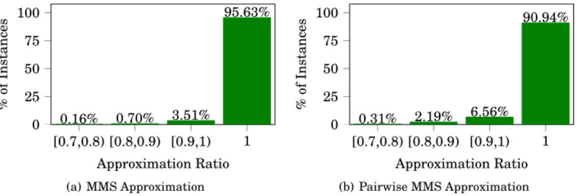
- MMS and Φ-pairwise MMS. We now evaluate it on these benchmarks (which, we re- iterate, it is not designed to optimize) using real-world data. Specifically, we use 1281 instances created so far through Spliddit’s “divide goods” application. The number of players in these instances ranges from 2 to 10, and the number of goods ranges from 3 to 93. Figures 1(a) and 1(b) show the histograms of the MMS and pairwise MMS approximation ratios, respectively, achieved by the MNW solution on these instances.

Most importantly, observe that the MNW solution provides every player her full

MMS (resp. pairwise MMS) guarantee, i.e., achieves the ideal 1-approximation, in

[0.7,0.8) [0.8,0.9) [0.9,1) 1 0

25 50 75 100

0.16% 0.70% 3.51%

95.63%

Approximation Ratio

% of Instances

(a) MMS Approximation

[0.7,0.8) [0.8,0.9) [0.9,1) 1 0

25 50 75 100

0.31% 2.19% 6.56%

90.94%

Approximation Ratio

% of Instances

(b) Pairwise MMS Approximation

Fig. 1. MMS and Pairwise MMS approximation of the MNW solution on real-world data from Spliddit.

more than 95% (resp. 90%) of the instances. Further, in contrast to the tight worst- case ratios of π

= Θ(1/ √

n) and Φ ≈ 0.618, the MNW solution achieves a ratio of at least 3/4 for both properties on all the real-world instances in our dataset.

5. IMPLEMENTATION

It is known that computing an exact MNW allocation is N P-hard even for 2 players with identical additive valuations, due to a simple reduction from the N P-hard prob- lem P ARTITION [Nguyen et al. 2013; Ramezani and Endriss 2010]. Our goal in this sec- tion is to develop a fast implementation of the MNW solution, despite this obstacle. An existing approach to maximizing the Nash welfare [Nongaillard et al. 2009] iteratively modifies an initial allocation to improve the Nash welfare at each step, but may return a local maximum that does not provide any fairness or efficiency guarantees. Instead, we use integer programming to find the global optimum in a scalable way. Note that most real-world instances are relatively small, but response time can be crucial. For example, Spliddit has a demo mode, where users expect almost instantaneous results.

Moreover, some instances are actually very large, as we discuss below.

Let us begin by recalling that the first step in computing an MNW allocation is to find a largest set of players S that can be given positive utility simultaneously. In the full version, we show that S can be computed easily by finding a maximum cardinality matching in an appropriate bipartite graph. The problem then reduces to computing an MNW allocation to the players in S. Hereinafter, we focus on this reduced problem.

Thus, without loss of generality we can assume that for the given set of players N , an MNW allocation will achieve positive Nash welfare.

Figure 2 shows a simple mathematical program for computing an MNW allocation.

The binary variable x

denotes whether player i receives good g. Subject to feasibility constraints, the program maximizes the sum of log of players’ utilities, or, equivalently, the Nash welfare. Note that this is a discrete optimization program with a nonlinear objective, which is typically very hard to solve.

Fortunately, we can leverage some additional properties of the problem that arise

in practice. Specifically, on Spliddit, users are required to submit integral additive

valuations by dividing 1000 points among the goods. This in turn ensures that the

utilities to the players will also be integral, and not more than 1000. In theory, this does

not help us: due to a known reduction from a strongly N P-complete problem — Exact

Cover by 3-Sets (X3C) — to the problem of computing an MNW allocation [Nguyen

et al. 2013], we cannot hope for a pseudopolynomial-time algorithm (i.e., a polynomial-

time algorithm for Spliddit-like valuations). In practice, however, this structure of the

valuations can be leveraged to convert the non-linear objective into a linear objective:

Maximize P

i∈N

log P

g∈M

x

· v

(g) subject to P

i∈N

x

= 1, ∀g ∈ M x

∈ {0, 1}, ∀i ∈ N , g ∈ M.

Fig. 2. Nonlinear discrete optimization program

x

log x Log

Segment Tangents (k, log k)

(k + 1, log(k + 1))

Fig. 3. The log function and its approximations Maximize P

i∈N

W

subject to W

6 log k +

log(k + 1) − log k

× h P

g∈M

x

· v

(g) − k i ,

∀i ∈ N , k ∈ {1, 3, . . . , 999}

P

g∈M

x

· v

(g) > 1, ∀i ∈ N P

i∈N

x

= 1, ∀g ∈ M x

∈ {0, 1}, ∀i ∈ N , g ∈ M.

Fig. 4. MILP using segments on the log curve

10 30 50

0 15 30

n

Time (s) MILP using

segments

Fig. 5. Running time of our MNW implementation

P

i∈N

P

t=2

(log t − log(t − 1)) · U

, where U

= I [ P

g∈M

x

· v

(g) > t] for player i ∈ N and t ∈ [1000] is an additional variable that can be encoded using two linear constraints. However, the introduction of 1000 · n additional binary variables makes this approach impractical even for fairly small instances.

We therefore propose an alternative approach that introduces merely n continuous variables and, crucially, no integral variables. The trick is to use a continuous variable W

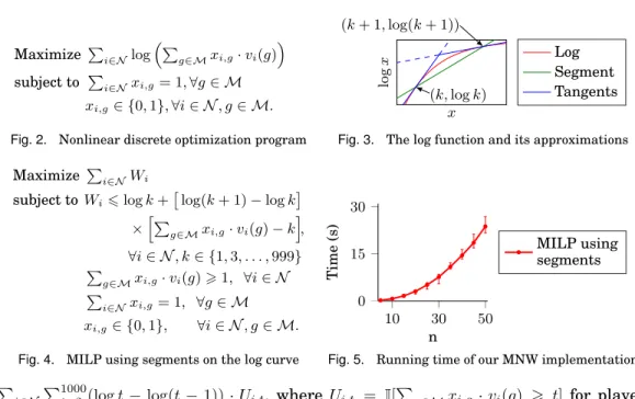
denoting the log of the utility to player i, and bound it from above using a set of linear constraints such that the tightest bound at every integral point k is exactly log k. This essentially replaces the log by a piecewise linear approximation thereof that has zero error at integral points. Figure 3 shows two such approximations of the log function (the red line): one that uses the tangent to the log curve at the point (k, log k) for each k ∈ [1000] (the blue lines), and one that uses segments connecting points (k, log k) and (k + 1, log(k + 1)) for each k ∈ {1, 3, . . . , 999} (the green line). Each tangent and each segment is guaranteed to be an upper bound on the log function at every integral point due to the concavity of log.

Importantly, note that the tightest upper bound at each positive integral point k is log k. These transformations do not work at k = 0, i.e., they do not ensure W

= −∞ if player i gets zero utility. However, recall that in our subproblem each player can achieve a positive utility. Hence, we eliminate this concern by adding the constraints that each player must receive value at least 1. We employ the transformation that uses segments as it requires half as many constraints (and, incidentally, runs nearly twice as fast). Figure 4 shows the final mixed-integer linear program (MILP) with only n continuous and n · m binary variables, which is key to the practicability of this approach.

To assess how scalable our implementation is, we measure its running time on uni- formly random Spliddit-like valuations, that is, uniformly random integral valuations that sum to 1000. We vary the number of players n from 5 to 50 in increments of 5, and keep the number of goods at m = 3 · n to match data from Spliddit, in which m/n ≈ 3 on average. The experiments were performed on a 2.9 GHz quad-core computer with 32

5

In fact, this transformation is useful in maximizing any concave function, or minimizing any convex func-

tion, and thus may be of independent interest.

GB RAM, using CPLEX to solve the MILPs. The indicator-variables-based approach failed to run within our time limit (60 seconds) even for 5 players. Figure 5 shows the running time (averaged over 100 simulations, with the 5th and 95th percentiles) of the MILP formulation from Figure 4. Satisfyingly, we can solve instances with 50 players in less than 30 seconds (whereas even the largest of the 1281 instances on Spliddit has 10 players). In fact, the algorithm solves every Spliddit instance in less than 3 seconds.

The largest real-world instance we have seen was actually reported offline by a Spliddit user. He needed to split an inheritance of roughly 1400 goods with his 9 sib- lings. Our implementation solves an instance of this size in roughly 15 seconds.

5.1. Precision Requirements

As our optimization program involves real-valued quantities (e.g., the logarithms), we must carefully set the precision level such that the optimal allocation computed up to the precision is guaranteed to be an MNW allocation. This is because an allocation that only approximately maximizes the Nash welfare may fail to satisfy the theoretical guarantees of an MNW allocation (Theorems 3.2 and 4.1, and Corollary 4.5).

Recall that our objective function is the log of the Nash welfare. Hence, the differ- ence between the objective values of an (optimal) MNW allocation and any suboptimal allocation is at least log(1000

) − log(1000

− 1) > 1/1000

− (1/2)/1000

, which can be captured using O(n) bits of precision. This simple observation can be easily formalized to show that there exists p ∈ O(n) such that if all the coefficients in the optimization program are computed up to p bits, and if the program is solved with p bits of precision (i.e., with an absolute error of at most 2

in the objective function), then the solution returned will indeed correspond to an MNW allocation. Crucially, p is independent of the number of goods. We expect the number of players n to be fairly small in everyday fair division problems. For example, as previously mentioned, on Spliddit more than 95% of the instances for allocating indivisible goods have n 6 3.

Nonetheless, if one’s goal is solely to find an allocation that is EF1 and PO, a con- stant number of bits of precision would suffice. This is because capturing differences in objective values that are at least log(1000

) − log(1000

− 1) — a constant — ensures that the resulting allocation is EF1 and PO, as we show below.

(1) EF1: Suppose the allocation is not EF1, and player i envies player j even after the removal of any single good from player j’s bundle. Then, our proof of Theo- rem 3.2 shows that we can increase the Nash welfare by moving a specific good from player j to player i. Because this operation does not alter the utilities to all but two players, it must increase the logarithm of the Nash welfare by at least log(1000

) − log(1000

− 1), which is a contradiction because our sensitivity level is sufficient to find this improvement.

(2) PO: Suppose the allocation is not PO. Then there exists an alternative allocation that increases the utility to at least one player without decreasing the utility to any player. This must increase the logarithm of the Nash welfare by at least log(1000) − log(1000 − 1) > log(1000

) − log(1000

− 1), which is again a contradiction because our sensitivity level is sufficient to find this improvement.

6. DISCUSSION

The goal of this paper is to advocate the Maximum Nash Welfare (MNW) solution for

the fair allocation of goods. While it is justified by elegant fairness (EF1) and efficiency

(PO) properties, these properties are not “sufficient” in and of themselves — they may

allow undesirable outcomes (an example is presented in the full version). What makes

the MNW solution compelling is that it provides intuitively fair outcomes, yet organi-

cally satisfies these formal fairness properties. Moreover, the MNW solution provides

a Θ(1/ √

n)-approximation to the MMS guarantee (Theorem 4.1), whereas an arbitrary EF1 and PO allocation only provides a 1/n-approximation (refer to the full version for a proof).

Throughout the paper we assumed that the goods are indivisible, but our results directly extend to the case where we have a mix of divisible and indivisible goods.

The MNW solution in this case can be seen as the limit of the MNW solution on the instance where each divisible good is partitioned into k indivisible goods, as k goes to infinity. Theorem 3.2 therefore implies that the MNW solution is envy free up to one indivisible good, that is, player i would not envy player j (who may have both divisible and indivisible goods) if one indivisible good is removed from the bundle of j. This provides an alternative proof for envy-freeness of the MNW/CEEI solution when all goods are divisible. The results of Section 4 also directly go through — in fact, the proof of the MMS approximation result (Theorem 4.1) already “liquidates” some of the goods as a technical tool. In the full version, we outline the modified and scalable version of the implementation described in Section 5, which we have deployed on Spliddit, that can allocate a mix of divisible and indivisible goods.

It is remarkable that when all goods are divisible, three seemingly distinct solution concepts — the MNW solution, the CEEI solution, and proportional fairness (PF) — coincide. This is certainly not the case for indivisible goods: while a CEEI solution and a PF solution may not exist, the MNW solution always does. Nonetheless, our investigation revealed that even for indivisible goods, the PF solution and the MNW solution are closely related via a spectrum of solutions, which offers two advantages.

First, it allows us to view the MNW solution as the optimal solution among those that lie on this spectrum and are guaranteed to exist. Second, it also gives a way to break ties — possibly even choose a unique allocation — among all MNW allocations. See the full version for a detailed analysis. This connection between MNW and PF raises an interesting question: Is it possible to relate the MNW solution to the CEEI solution when the goods are indivisible?

Finally, we have not addressed game-theoretic questions regarding the manipulabil- ity of the MNW solution. The reason is twofold. First, there are strong impossibility re- sults that rule out reasonable strategyproof solutions. For example, Schummer [1997]

shows that the only strategyproof and Pareto optimal solutions are dictatorial — which means they are maximally unfair, if you will — even when there are only two players with linear utilities over divisible goods; clearly a similar result holds for indivisible goods (at least in an approximate sense).

Second, we do not view manipulation as a major issue on Spliddit, because users are not fully aware of each other’s preferences (they submit their evaluations in private), and — presumably, in most cases — have a very partial understanding of how the algorithm works.

REFERENCES

M. Aleksandrov, H. Aziz, S. Gaspers, and T. Walsh. 2015. Online Fair Division: Analysing a Food Bank Problem. In Proc. of 24th IJCAI. 2540–2546.

G. Amanatidis, E. Markakis, A. Nikzad, and A. Saberi. 2015. Approximation Algorithms for Computing Maximin Share Allocations. In Proc. of 42nd ICALP. 39–51.

K. J. Arrow and M.D. Intriligator (Eds.). 1982. Handbook of Mathematical Economics. North- Holland.

H. Aziz, S. Gaspers, S. Mackenzie, and T. Walsh. 2015. Fair assignment of indivisible objects under ordinal preferences. Artificial Intelligence 227 (2015), 71–92.

6

In theory, one can hope to circumvent this result by making manipulation computationally hard [Bartholdi

et al. 1989]. This is almost surely true (in the worst-case sense of hardness) for the MNW solution, where

even computing the outcome is hard.