A Nonparametric Analysis of Regional Unemployment Dynamics in Britain

A Nonparametric Analysis of Regional Unemployment Dynamics in Britain

Marco

Bianchi

Gyl

Zoega

Bank of England Birkbeck College Monetary Analysis Department of Economics Threadneedle Street Gresse Street London, EC2R 8AH London, W1P 2LL

Abstract.

This paper estimates the probability distribution of relative county unemployment in Britain for the years 1981-1995. We nd that the distribution is unimodal in all years, with a falling variance between 1989 and 1994. We use bootstrap methods to determine critical values for the two tails of the distribu- tion, and analyse intra-distribution dynamics. An unemployment transition is dened as a move between a tail and the centre of the distribution (and vice ver- sa). We calculate transition probabilities and nd that the probability of leaving any given state is very low. We also nd that high (low) unemployment regions have a higher probability of entering a state of lower (higher) unemployment than a state of higher (lower) unemployment.

Keywords: Regional unemployment, panel data, asymmetric eects in the per- sistence of transition dynamics, nonparametric analysis.

JEL Classication: E24, R12, C14.

We thank Sigbert Klinke, Danny Quah, Ron Smith and Howard Wall for comments and suggestions. The data and the programs (written in the GAUSS programming language) are available upon request from the authors. The rst author aknowledges the hospitality of the Institut fur Statistik und Okonometrie at Humboldt University, Berlin. The usual disclaimer applies. The views expressed in this paper do not necessarily reect those of the Bank of England.

1 Introduction

In this paper we use nonparametric methods to describe the county-level dynamics of un- employment in Britain. We want to analyse rst the distribution of relative unemployment to know whether it is multimodal. The high-unemployment areas of Scotland, Wales and northern England are often contrasted with the lower unemployment areas in the south counties in those regions might form a group separate from the rest. Secondly, we would like to know whether the variance of unemployment across counties has changed during recent years. A falling variance could either imply that high-unemployment counties are recovering due to migration and capital movements, or that the geographical distribution of shocks has changed over time ( -convergence, see Barro and Sala-i-Martin, 1995). Finally, we are interested in assessing the relative fortunes of dierent counties by identifying those enjoying persistent prosperity and those suering persistent unemployment. We want to know, for example, whether it is more dicult to recover from a (relative) depression than it is to fall from (relative) prosperity.¹ (

-convergence).

There exists a substantial literature studying regional unemployment persistence for dierent countries. Blanchard and Katz (1992) studied the US, Jimeno and Bentolila (1995) Spain, and Decressin and Fatas (1995) European regions. The results suggest that migration plays a key role in the US so that regional labour demand shocks have only a small transitory eect on regional unemployment. In Europe, however, it is through changes in labour force participation² that employment is aected in the short run, and through migration in the long run. There is no long-run eect on unemployment in either case. Spain is an exception, according to Jimeno and Bentolila unemployment responds more to labour demand shocks, and its changes last longer.

In Bianchi and Zoega (1996), we use similar conventional methodology to look at regional unemployment data for Britain in order to measure the persistence of relative unemployment rates in the ten regions, and the response to changes in regional labour demand. We measure steady-state unemployment rates for each of the regions, and the speed of adjustment towards these steady-states following regional shocks. Regional unemployment appears either to be nonstationary or if there is any convergence over time, it is extremely slow.

The point estimates imply that if unemployment in any one region is 5% higher than its steady-state value (that is 500 basis points higher), the unemployment rate will fall by only 65 basis points in the rst year (0.65%) and that it would take more than 12 years for unemployment to return to steady state. If the rate started out 10% higher than the steady state value, it would take more than 17 years to return to the steady-state value. Thus, British regional labour markets appear to be much less integrated than labour markets in continental Europe and in the US. In the latter, migration eliminates unemployment dierentials within 4-6 years.

1Counties may possibly get trapped at very high levels of unemployment if some of the adjustment mechanisms { migration and capital movements { break down.

2This includes early retirement and disability pension.

These results lend support to earlier studies of regional labour markets in Britain (see Blackaby and Manning, 1981 Hughes and McCormick, 1987, 1994 Evans and McCormick, 1994 Pissarides and McMaster, 1989 Pissarides and Wadsworth, 1990 Jackman and Savouri, 1992 and Pencavel, 1994). Pissarides and McMaster, using interregional migra- tion data, nd that migration responds very slowly to dierences in regional unemployment.

Their results imply that it can take more than twenty years for an unemployment dierential in a depressed region to disappear. Evans and McCormick nd an integrated labour market for non-manuals, where migration equalizes regional unemployment rates, but they nd the market for manuals to be localized with persistent unemployment dierentials across regions, and hardly any interregional migration in response to unemployment dierences.

The objective of this paper is to look more closely at regional labour market dynamics in Britain using non-parametric methods. In doing so we attempt to provide an alternative methodology for analysing regional developments. We use kernel density estimation to estimate the probability distribution of relative unemployment rates across 64 counties for the years 1981-1995. This enables us to test for the existence of modes in the distribution and to observe changes in the variance of relative unemployment during this period. Also, we look at movements of counties within the distribution between years and calculate transition probabilities of leaving states of dierent relative unemployment.

The organization of this paper is as follows. Section 2 describes the statistical framework (our denitions of shocks and persistence, nonparametric density estimation, construction of bootstrap condence intervals and classication analysis, the analysis of intra{distribution dynamics, etc). Section 3 has the empirical results. Section 4 concludes.

2 The Statistical Framework

2.1 Intra-distribution Dynamics

We have longitudinal data on unemployment rates³ for

n

= 64 counties from 1981 to 1995.

We are interested in establishing empirical facts about shocks to their unemployment ratios as well as the persistence of these shocks. To this end we construct a formal statistical denition of shocks based on classication analysis and the concept of intra-distribution dynamics.

We denote by

x

i the ratio of unemployment in county

i

to the aggregate British unem- ployment rate, and by

f

(

x

) its probability distribution at time

t

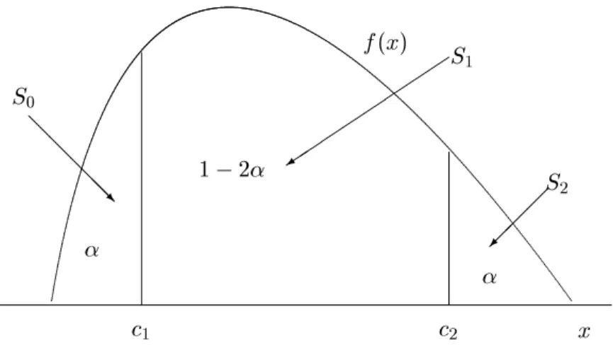
. In Figure 1 it is assumed that we know the probability distribution of the data and we x a value of

to dene the area in each tail of the distribution. This allows us to identify two critical values,

c

1 and

3These are annual averages. The rates are calculated by expressing the number of unemployed claimants as a percentage of the estimated total workforce (the sum of of unemployed claimants, employees in employ- ment, self-employed, HM forces and participants on work-related training programmes). Source: Employ- ment Gazzette, various issues.

c

2, on the real line such that

Z c¹

;1

f

(

x

)

dx

=^Z_c⁺¹

2

f

(

x

)

dx

=

:

Then, we dene county

i

to be in the state of:

\Low Unemployment" =

S

0 ^{() ;1}

< x

i

c

1,

\Average Unemployment" =

S

1 ⁽⁾

c

1

< x

i

c

2,

\High Unemployment" =

S

2 ⁽⁾

c

2

< x

i

<

¹.

We construct an indicator variable for county

i

at time

t

,

I

i(

t

), which takes the values 0,1 and 2 (respectively, the states of low, average and high unemployment), i.e.:

I

i(

t

) =

8

>

<

>

:

0 if

x

i ²

S

0

1 if

x

i ²

S

1

2 if

x

i ²

S

2

:

⁽¹⁾

By doing the above classication analysis for each county (

i

= 1

:::n

) and every year (

t

= 1981

:::

1995), we are able to focus on intra-distribution dynamics. We now have the following denition:

Denition:

a county

i

is hit by a positive shock at time

t

if

I

i(

t

+ 1)

< I

i(

t

) it is aected by a negative shock if

I

i(

t

+ 1)

> I

i(

t

).

is

2.2 Nonparametric Density Estimation and Classication Analysis

Given the data and a positive value

1

=

3, inference on intra-distribution dynamics requires us to know the true probability

f

(

x

). As a matter of fact, the true probability is never known, but we can replace

f

(

x

) by a non-parametric estimate

f

^h(

x

) = (

nh

)^;1Xn

i=1

K

x

^;

x

i

h

= (

nh

)^;1Xn

i=1

K

(

u

)

(2)

where

h >

0 is the bandwidth (governing the degree of smoothness of the estimate, with larger values of

h

producing a smoother density estimate) and

K

(

u

) = 1

=

^p2 exp(^;1

=

2

u

²) being the Gaussian kernel (see Silverman, 1986 Hardle, 1990).

In this way, we obtain estimates ^

c

1and ^

c

2 of the critical values whereas our classication analysis depends on the \true" critical values

c

1 and

c

2. We therefore construct condence intervals for

c

1 and

c

2, i.e.

Pr(

c

₁

c

1

c

1) = Pr(

c

₂

c

2

c

2) =

c

(3) where

c

is the coverage probability (for example

c

= 0

:

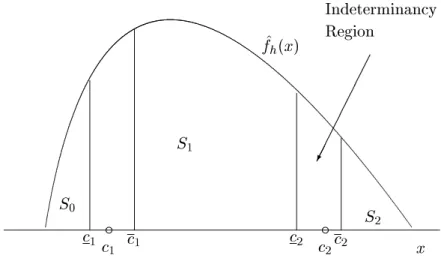
80).

The situation is summarised in Figure 2, which shows two regions of indeterminancy if

x

i is in the interval

c

1

c

1] or

c

2

c

2], it is unknown whether county

i

should be allocated to state

S

0 or

S

1. Counties with unemployment ratios smaller than

c

₁, however, are allocated to the state of low unemployment with probability

c

, and counties with unemployment ratios bigger than

c

2 are allocated to the state of high unemployment. In other words, with probability

c

, a county

i

with

c

1

< x

i

< c

₂ at time

t

but

x

i

> c

2at time

t

+1, can be dened to have been aected by a negative shock at time

t

. However, for a county

s

in the same situation at time

t

(that is with

c

1

< x

s

< c

₂) and with

x

s

> c

₂ but

x

s

< c

2 at time

t

+ 1, the switch from

S

1 to

S

2 could be generated by noise rather than by a genuine negative shock.⁴

Given the above considerations, we dene the ve areas in the distribution according to

I

i(

t

) =

8

>

>

>

>

>

<

>

>

>

>

>

:

0 if

x

i ²

S

0

5 if

x

i ²(

c

1

c

1] 1 if

x

i ²

S

1

5 if

x

i ²(

c

₂

c

2] 2 if

x

i ²

S

2

(4)

where 5 represents the code of the indicator in the regions of indeterminancy (regardless of whether we are in between

S

0 and

S

1, or

S

1 and

S

2).

As the density of the data is estimated nonparametrically, we use the bootstrap ap- proach to construct the condence intervals. This means that given an optimal bandwidth

h

,⁵ calculated using the plug-in method of Sheather and Jones (1991), we resample with replacement from the original data. Due to an eect of the Gaussian kernel, bootstrap samples drawn from

f

h have a variance larger than the sample variance of the data, so the following transformation is required (see Efron and Tibshirani, 1993, page 231 and 234 for details)

x

_i = "

y

+ (1 +

h

²^²)^;1=2(

y

_i ^;

y

" +

he

i)

i

= 1

:::n

(5) where

y

= (

y

₁

:::y

_n)⁰ are sampled with replacement from

x

= (

x

1

:::x

n)⁰ "

y

= mean(

y

), ^² is the sample variance of

x

and

e

i are standard normal variables generated by the computer.⁶

The construction of the condence intervals and the implementation of the classication analysis can be summarised as follows:

4A more complete treatment of the problem would require a joint, rather than pointwise, con dence interval for the quantiles across time.

5By optimal we mean here the minimisation of the trade-o between the bias and the variance of the estimator in a AMISE (asymptotic mean integrated squared error) sense. See for example Marron, Jones and Sheather (1992), Sheather and Jones (1991), Bianchi (1995a).

6It can be shown (see Efron and Tibshirani, 1993, page 234) that if^y is sampled with replacement from

x,^e= (e¹:::en)⁰ has a standard normal distribution andhis xed, then: i)^{r y} +h^e is distributed according to ^fh ii)^r has the same mean as^y and variance ^²+h² iii)^x = (x¹:::xn)⁰ de ned as in equation (5) has the same mean as^r but variance approximately equal to ^².

0. select bandwidth

h

from the sample data using a data{driven bandwidth selector (for example, Sheather and Jones, 1991)

1. draw

B

bootstrap samples

y

of size

n

from

x

by sampling with replacement 2. dene the rescaled bootstrap samples

x

as in (5)

3. for each boostrap sample

x

, estimate the density ^

f

h(

x

) and, given

, obtain the critical value pairs^f^

c

₁(

b

)

c

^₂(

b

)^g_Bb=1

4. derive the condence limits

c

_k,

c

kby taking the^f(

B

^;

Bc

)^g-th and the^f

Bc

^g-th largest of the

B

replicates ^

c

_k,

k

= 1

2

5. construct the indicator ^

I

i(

t

) as in (4), for

i

= 1

:::n

and

t

= 2

::: T

(this gives an

n

(

T

^;1) design matrix with elements 0, 1, 2 or 5)

6. at

t

= 1, x ^

c

k = median^f^

c

_k(

b

)^g_Bb=1, for

k

= 1

2, and classify the

i

-th county in

S

0 if

x

i

c

^1,

S

2 if

x

i

> c

^2 or

S

1 otherwise

7. for

t

= 2

::: T

, allocate counties falling in the indeterminancy regions to the same state they were at

t

^;1 this gives an

n

T

design matrix,

D

, with elements 0, 1, or 2.

The design matrix

D

summarises most information on intra-distribution dynamics which is relevant for making inference about transition probabilities (these describe the probability of a county leaving one state of relative unemployment for another). For these, we analyse the columns of the matrix at each point in time, from

t

= 2

:::T

, we count the proportion of counties that moved from

S

l to

S

m, for

lm

= 1

2

3, between

t

^;1 and

t

. This will allow us to address the issue of

-convergence: this implies that counties with high (low) relative unemployment should have higher transition probabilities to states of lower (higher) relative unemployment than counties with higher (lower) unemployment rates.

To address the issue of -convergence, nonparametric density estimation can be used rst to test for the number of modes in the true probability distribution

f

(

x

). It is of in- terest whether the counties can be grouped into high- and low-unemployment areas in that way. Thus it is possible that certain regions of the country have high mean unemployment while others have a much lower mean rate. A formal test for unimodality can easily be im- plemented by the bootstrap method, as discussed in Silverman (1981, 1983, 1986) and Efron and Tibshirani (1993).⁷ Having detected the number of modes, we then measure changes in the variance across the counties over time. If the variance is falling over time, we have a case of -convergence. This might either suggest the operation of adjustment mechanisms, such as inter-county labour migration, or changes in the geographical distribution of shocks.

Finally, we can also record the dating of the dierent shocks and, by looking at the kernel density estimates for these dates, check whether positive and negative shocks occurred at dierent times.

7A summary of the procedure is reported in the Appendix. See Bianchi (1997) for an application to per-capita GNP series.

2.3 Generalization and Model Selection

Before turning to the empirical analysis of unemployment data, we briey discuss the advan- tages of our statistical methodology. We also generalize the model to an arbitrary number of states and discuss the choice of our model's parameters.

The advantage of non-parametric methods in the context of our analysis is clearly exi- bility, in so far that virtually any shape of the density can be accounted for by the method.

Regardless of whether the empirical distribution is well approximated by a Gaussian dis- tribution or has fat tails, skewness and/or kurtosis, non-parametric density estimation will automatically estimate the dierent shapes. Using parametric methods, on the other hand, one would have to try a variety of parametric families and choose the family which best ts the data in each year. Moreover, it is very unlikely that the way nonparametrics are implemented may inuence the results it is well known that the choice of the kernel func- tion is not of great signicance and that the choice of the bandwidth need not be subjective because data driven methods with optimal statistical properties are readily available | such as for example the plug-in method of Sheater and Jones (1991).⁸

However, the choice of the number of unemployment states and the areas in the tails of the distribution deserves a more detailed explanation. The analysis presented in previous sections is based, in fact, on a threefold classication of unemployment (high, low, average) with

= 0

:

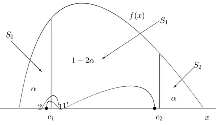
30. This is only for expositional purposes, as the underlying model can be generalized to include a higher number of states with dierent probability areas in each state. The generalization requires us to carefully consider two extreme situations depicted in Figure 3. The rst situation is that of a county moving from a state of low (high) to a state of average unemployment in a given time period | a movement from `a' to `b' in Figure 3 | to revert back to the low (high) unemployment state next period | movement from `b' to `c'. In both cases, we have very small movements in the neighbourhood of the cut point

c

1 (

c

2) which, intuition suggests, should not be recorded as genuine state transitions.

Such spurious transitions will not be detected in our framework thanks to the construction of the indeterminancy regions obtained from bootstrap condence intervals. However, when a county jumps, within the state of average unemployment from a level close to

c

1 to a level close to

c

2, this may be a cause for concern. The movement from `d' to `e' in Figure 3, in fact, should be detected as a truly genuine transition in our analysis of intradistribution dynamics but it may not be detected in practice.⁹ In the context of a three-state model, the risk of failing to detect a large movement of this kind is higher the lower the value of

. For this reason, the largest possible value of

minimising the distance between the two cut points

c

1and

c

2,

= 1

=

3, should be selected to minimise this risk. A better alternative may be to allow for a higher number of unemployment states, such as for example ve (lower, low, average, high, higher) instead of three.

To summarise, we can represent our general statistical model by the parameters' set

8The method of Sheater and Jones is statistically optimal in the sense of minimising the mean square error of the estimator. Marron et al (1992) report the results of an extensive simulation study showing the excellent performance of the SJ bandwidth selector in small samples.

9We thank Danny Quah for raising this point.

M

= ^f

hS

1

:::

S

c

^g, where

h

is the bandwidth for the non-parametric density esti- mate of (relative) unemployment rates

S

is the number of unemployment states

s is the probability area for the

s

-th state, with ^P_Ss=1

s = 1 and

c

is the coverage probability for the condence intervals. It is clear from the discussion above that there is a natural choice for most of our parameters, which is as follows:

h

=

h

SJ, where

h

SJ is the band- width selected by the method of Sheater and Jones (1991) and

1 =

2 =

3 = 1

=

3 or

1 =

2 =

3 =

4 =

5 = 1

=

5. The choice of the coverage probability

c

for the con- struction of condence intervals remains more subjective, as any number between 0.80 and 0.95 could be selected. Nevertheless, the closer the value of

c

is to unity, the wider the condence interval for the cut points. A value of

c

equal to 0.95 or 0.90 may lead therefore to an overlap of the indeterminancy regions. In our application, we have selected a value of

c

= 0

:

80 to avoid this.

3 Empirical Results

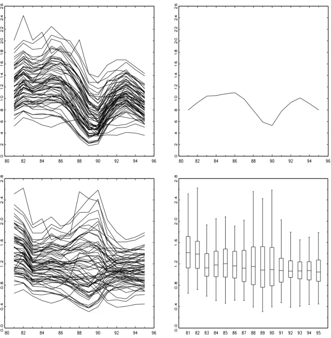
Following the statistical methodology described in Section 2, we take a look at the levels of unemployment in 64 counties from 1981-1995. The data are shown in Figure 4 (top-panels) the county unemployment rates in the left-hand side panel, the aggregate unemployment rate in the right-hand side panel. Because we are interested in looking at the unemployment problem in dierent counties relative to the national aggregate, the counties unemployment rates are divided by the UK aggregate this leads to the series plotted in the bottom-left panel of Figure 4.¹⁰

The bottom-right panel shows the boxplot representation of these series, which presents the distribution of the data in dierent years. A drop in the median of the distributions (represented by the horizontal line in the box) can be noticed after 1982 to a value closer to unity also there is a signicant reduction in the dispersion of the distributions (represented by the size of the box) over the last 4-5 years. For most years, the densities appear somewhat skewed towards large values, but with very few outliers.

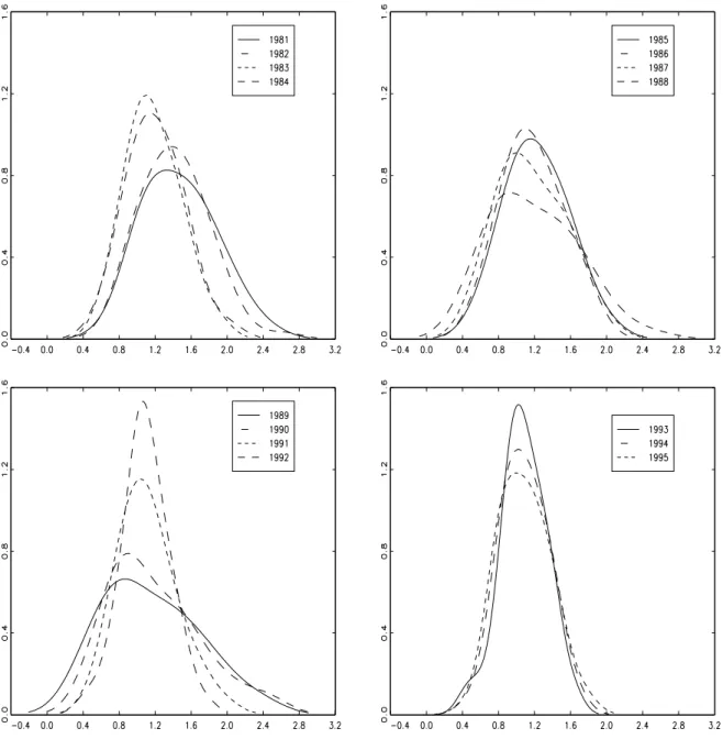
For the unemployment ratios, the bandwidths selected by the method of Sheather and Jones (see Table in the Appendix) give the density estimates shown in Figure 5. The probability distribution is unimodal in all years.¹¹ There is a clearly visible fall in the mean (relative) unemployment in the early 1980s, and also in the variance of the distribution in the early 1990s. The latter is presumably caused by the uncharacteristically deep recession in the South. The fall in the variance around 1990 and the increase in the rst half of 1990's is a reection of the regional distribution of shocks. Both the recovery in the late 1980's and the recession in the 1990's were concentrated in the South.

10We could have used here absolute unemployment rates rather than relative unemployment rates and this would not change the results of our analysis. In fact, densities of absolute and relative unemployment rates are identical, apart from a scaling factor. In any given year the absolute unemployment rate can be derived from the relative rate by multiplying every observations by the average British unemployment rate.

But this would just shift the mode of our density.

11Formal multimodality tests using nonparametric kernel density estimation and the bootstrap reject multimodality in all years | see the results reported in the Appendix.

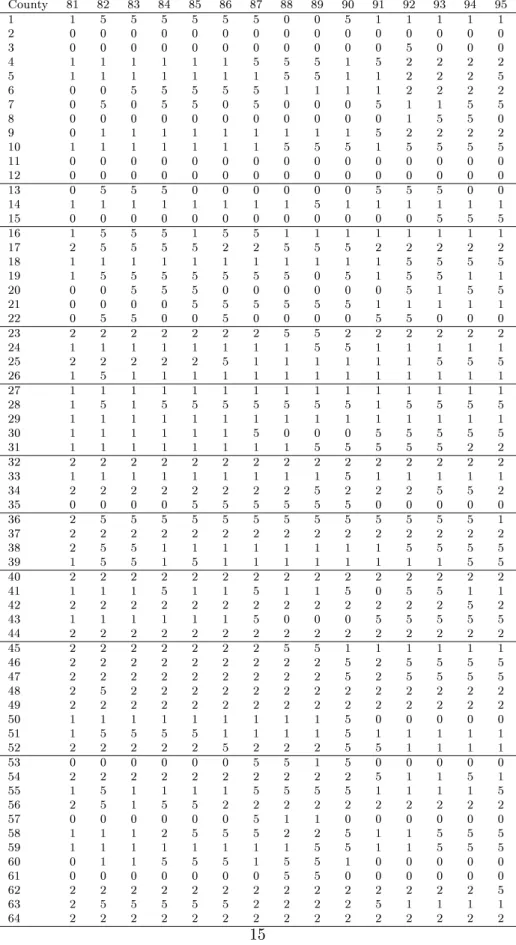
The densities, together with a xed value for the area in the tails of the distribution,

= 1

=S

with

S

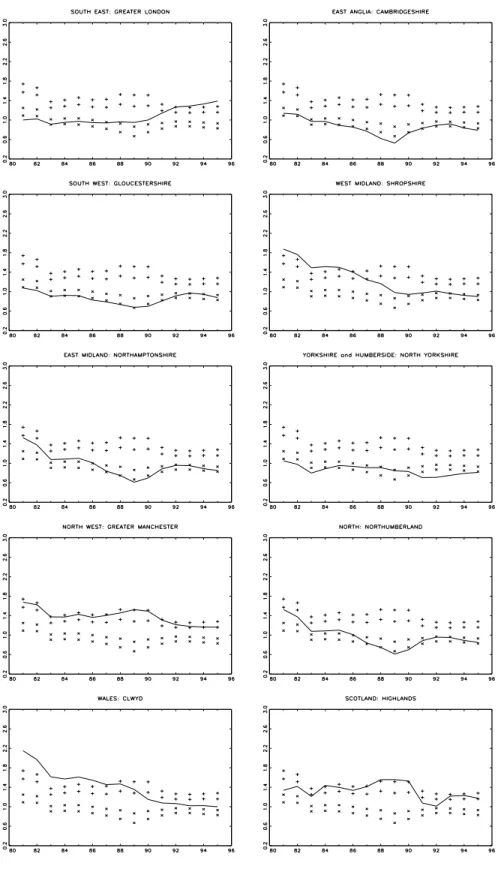
= 3, give the intra-distribution dynamics in Table 1. Figure 6 plots the intra-distribution dynamics for 10 counties,¹² one from each of the 10 regions. The rst panel shows the intra-distribution dynamics for Greater London. London starts out in the area of low unemployment but in 1983 enters the zone of indeterminancy between \low" and

\normal" unemployment. In 1988 it enters the area of normal unemployment and nally in 1993 the area of high unemployment.

positive shocks

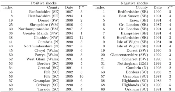
Figure 7 shows the density estimate of the dates of the shocks. It appears that positive shocks occurred more frequently in the period between 1985 and 1993 (and, within this period, more frequently in 1989), whereas most negative shocks (which particularly aected South-East counties) occurred in 1981 and 1991.

It is also interesting to examine whether it is more likely or less likely for a given county nding itself in the left-tail of the distribution to move to the centre than for a similar county in the high-unemployment right-tail of the distribution. The matrix in Table 3 has the transition probabilities between the three states, which is calculated as the average probability over the 14 years. The rst row refers to

S

0, the second row to

S

1, and the third to

S

2. The rst number in row 1 shows the probability that a county in region

S

0 in year

t

^;1 will remain in that same state in year

t

. The second number is the probability of moving from state

S

0 to

S

1 and the last number is the probability of moving to state

S

2.

We see that changes in the relative county unemployment rates are very persistent. The probability that a county stays in the current state between any two years is 92.5% for

S

0, 95.8% for

S

1 and 97.2% for state

S

2. The probability of getting out of a bad state,

S

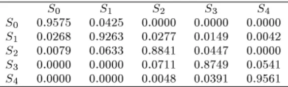
2, is only 3.3% and about the same as the probability of getting out of the good one, 3.2%.

Table 4 has the analogous transition probabilities for the case of ve states with

S

= 5 and

= 0

:

2. Again we nd that relative unemployment is very persistent. However, we also nd that a county with a high (low) level of relative unemployment has a higher probability of moving to a state of lower (higher) unemployment. This implies

-convergence. For example, a county nding itself in the second highest unemployment state has a probability of 2.68% of moving to the highest state and a probability of 4.68% of moving to one of the three states with lower unemployment. Similarly, a county in the second lowest state of unemployment has a probability of 5.41% of moving to the state of lower unemployment and a probability of 7.11% of moving to a state of higher unemployment.

We conclude that the key results of our analysis of intra-distribution dynamics | the persistence of relative unemployment | is not sensitive to our choice of the number of states. However, using ve states allows us to take a closer look at the dynamics.¹³

because

12We would like to point out that the seven metropolitan districts are strictly speaking not counties in the sense that each has more than one local government.

13We also derived the transition probabilities using coverage probabilities (c) of 0.85 and 0.90, with very similar results.

4 Conclusions

This paper has used nonparametric methods to analyse unemployment persistence. We used data on unemployment at the county level in Britain from 1981-1995 to test for the number of modes in the probability distribution across the counties. We found the distribution to be unimodal in every year. While in any given year there are counties with very high and very low unemployment rates, we do not detect signicant subgroups in the data with either high or low rates.

By constructing condence intervals for quantiles (critical values) in the density which leave 33% of observations in each tail of the distribution, we analysed the persistence of movements of counties between the three states of unemployment (low, average, high), corresponding to the middle and the two tails of the distribution. We found that the transition probabilities were the same for the two tails. We also found that positive shocks mainly occurred in the period 1985-1993, whereas negative shocks, which mostly aected counties in the South-East, occurred in 1981 and, particularly, in 1991.

The transition probabilities conrmed a high degree of persistence of changes in rela- tive unemployment. Thus the probability that a county nding itself in a state of high unemployment will stay in that state in the following year is around 97%. This implies that the regional adjustment mechanisms of inter-county migration and capital movements are very weak. When using ve states of unemployment instead of three, we again found unemployment persistence, but also a tendency for high unemployment regions to recover and low unemployment regions to experience rising unemployment. This presents evidence in favour of weak

-convergence.

1^;2

f

(

x

)

c

1

c

2

@

@

@

@

@ R

S

0

+

S

1

;

;

;

S

2

x

Figure 1: Classication analysis.

f

^h(

x

)

c

1

c

2

x

S

1

S

0

S

2

Indeterminancy Region

c c

c

1

c

1

c

2

c

2

Figure 2: Classication analysis with indeterminancy regions.

1^;2

f

(

x

)

c

1

c

2

@

@

@

@

@ R

S

0

+

S

1

;

;

;

S

2

x

s 1 s

2 1⁰

Figure 3: Example of two extreme cases in our classication analysis.

Figure 4: Top: Unemployment rates in percentage points in 64 UK counties (left) and in the UK (right), from 1981 to 1995. Bottom: unemployment ratios (left) with the corresponding boxplots (right).

Figure 5: Kernel density estimates for the unemployment ratios of 64 counties in dierent years using the bandwidths reported in the Appendix.

County 81 82 83 84 85 86 87 88 89 90 91 92 93 94 95

1 1 5 5 5 5 5 5 0 0 5 1 1 1 1 1

2 0 0 0 0 0 0 0 0 0 0 0 0 0 0 0

3 0 0 0 0 0 0 0 0 0 0 0 5 0 0 0

4 1 1 1 1 1 1 5 5 5 1 5 2 2 2 2

5 1 1 1 1 1 1 1 5 5 1 1 2 2 2 5

6 0 0 5 5 5 5 5 1 1 1 1 2 2 2 2

7 0 5 0 5 5 0 5 0 0 0 5 1 1 5 5

8 0 0 0 0 0 0 0 0 0 0 0 1 5 5 0

9 0 1 1 1 1 1 1 1 1 1 5 2 2 2 2

10 1 1 1 1 1 1 1 5 5 5 1 5 5 5 5

11 0 0 0 0 0 0 0 0 0 0 0 0 0 0 0

12 0 0 0 0 0 0 0 0 0 0 0 0 0 0 0

13 0 5 5 5 0 0 0 0 0 0 5 5 5 0 0

14 1 1 1 1 1 1 1 1 5 1 1 1 1 1 1

15 0 0 0 0 0 0 0 0 0 0 0 0 5 5 5

16 1 5 5 5 1 5 5 1 1 1 1 1 1 1 1

17 2 5 5 5 5 2 2 5 5 5 2 2 2 2 2

18 1 1 1 1 1 1 1 1 1 1 1 5 5 5 5

19 1 5 5 5 5 5 5 5 0 5 1 5 5 1 1

20 0 0 5 5 5 0 0 0 0 0 0 5 1 5 5

21 0 0 0 0 5 5 5 5 5 5 1 1 1 1 1

22 0 5 5 0 0 5 0 0 0 0 5 5 0 0 0

23 2 2 2 2 2 2 2 5 5 2 2 2 2 2 2

24 1 1 1 1 1 1 1 1 5 5 1 1 1 1 1

25 2 2 2 2 2 5 1 1 1 1 1 1 5 5 5

26 1 5 1 1 1 1 1 1 1 1 1 1 1 1 1

27 1 1 1 1 1 1 1 1 1 1 1 1 1 1 1

28 1 5 1 5 5 5 5 5 5 5 1 5 5 5 5

29 1 1 1 1 1 1 1 1 1 1 1 1 1 1 1

30 1 1 1 1 1 1 5 0 0 0 5 5 5 5 5

31 1 1 1 1 1 1 1 1 5 5 5 5 5 2 2

32 2 2 2 2 2 2 2 2 2 2 2 2 2 2 2

33 1 1 1 1 1 1 1 1 1 5 1 1 1 1 1

34 2 2 2 2 2 2 2 2 5 2 2 2 5 5 2

35 0 0 0 0 5 5 5 5 5 5 0 0 0 0 0

36 2 5 5 5 5 5 5 5 5 5 5 5 5 5 1

37 2 2 2 2 2 2 2 2 2 2 2 2 2 2 2

38 2 5 5 1 1 1 1 1 1 1 1 5 5 5 5

39 1 5 5 1 5 1 1 1 1 1 1 1 1 5 5

40 2 2 2 2 2 2 2 2 2 2 2 2 2 2 2

41 1 1 1 5 1 1 5 1 1 5 0 5 5 1 1

42 2 2 2 2 2 2 2 2 2 2 2 2 2 5 2

43 1 1 1 1 1 1 5 0 0 0 5 5 5 5 5

44 2 2 2 2 2 2 2 2 2 2 2 2 2 2 2

45 2 2 2 2 2 2 2 5 5 1 1 1 1 1 1

46 2 2 2 2 2 2 2 2 2 5 2 5 5 5 5

47 2 2 2 2 2 2 2 2 2 5 2 5 5 5 5

48 2 5 2 2 2 2 2 2 2 2 2 2 2 2 2

49 2 2 2 2 2 2 2 2 2 2 2 2 2 2 2

50 1 1 1 1 1 1 1 1 1 5 0 0 0 0 0

51 1 5 5 5 5 1 1 1 1 5 1 1 1 1 1

52 2 2 2 2 2 5 2 2 2 5 5 1 1 1 1

53 0 0 0 0 0 0 5 5 1 5 0 0 0 0 0

54 2 2 2 2 2 2 2 2 2 2 5 1 1 5 1

55 1 5 1 1 1 1 5 5 5 5 1 1 1 1 5

56 2 5 1 5 5 2 2 2 2 2 2 2 2 2 2

57 0 0 0 0 0 0 5 1 1 0 0 0 0 0 0

58 1 1 1 2 5 5 5 2 2 5 1 1 5 5 5

59 1 1 1 1 1 1 1 1 5 5 1 1 5 5 5

60 0 1 1 5 5 5 1 5 5 1 0 0 0 0 0

61 0 0 0 0 0 0 0 5 5 0 0 0 0 0 0

62 2 2 2 2 2 2 2 2 2 2 2 2 2 2 5

63 2 5 5 5 5 5 2 2 2 2 5 1 1 1 1

64 2 2 2 2 2 2 2 2 2 2 2 2 2 2 2

Table 1: Results of our classication analysis by nonparametric density estimation with bandwidths

h

reported in the Appendix,

S

= 3,

= 1

=

3,

c

= 0

:

80 and

B

= 1000. Note: 5

15

Figure 6: Plot of unemployment ratios for 10 counties. Note: the symbols mark the indeterminancy region for

c

1 the + symbols represent the indeterminancy region for

c

2.

Positive shocks Negative shocks

Index County Date Y⁺ Index County Date Y^;

1 Bedfordshire (SE) 1987 3 1 Bedfordshire (SE) 1990 5 8 Hertfordshire (SE) 1994 1 4 East Sussex (SE) 1991 4

19 Dorset (SW) 1988 2 5 Essex (SE) 1991 4

25 Shropshire (WM) 1986 9 6 Gr. London (SE) 1987 4

30 Northamptonshire (EM) 1987 8 6 Gr. London (SE) 1991 4 36 Greater Manch (NW) 1994 1 7 Hampshire (SE) 1991 4 38 Cheshire (NW) 1983 12 8 Hertfordshire (SE) 1991 3

41 Cumbria (N) 1990 3 9 Isle of Wight (SE) 1981 10

43 Northumbershire (N) 1987 8 9 Isle of Wight (SE) 1991 4

45 Clwyd (Wales) 1989 6 19 Dorset (SW) 1990 5

50 Powys (Wales) 1990 5 20 Gloucerstershire (SW) 1992 3

52 West Glam (Wales) 1991 4 21 Somerset (SW) 1990 5

53 Borders (SC) 1990 5 31 Nottingham (EM) 1993 2

54 Central (SC) 1991 4 41 Cumbria (N) 1993 2

56 Fife (SC) 1982 3 53 Borders (SC) 1988 2

56 Fife (SC) 1985 10 57 Granpian (SC) 1987 2

57 Grampian (SC) 1989 6 58 Highlands (SC) 1983 7

60 Orkneys (SC) 1990 5 58 Highlands (SC) 1990 5

63 Tayside (SC) 1991 4 60 Orkneys (SC) 1981 9

Table 2: Summary results from the classication analysis concerning the dating and the persistence of shocks. Legend: SE = South East SW = South West WM = West Midlands EM = East Midlands N = North NW = North West SC = Scotland.

Dating of Shocks

Density

1980 1985 1990 1995

0.00.020.040.060.080.100.120.14

Positive Negative

Figure 7: Density estimate of the dating of positive and negative shocks. Note:

h

= 6 for the density estimate of both positive and negative shocks.

S⁰ S¹ S² S⁰ 0.968 0.032 0.000 S¹ 0.027 0.949 0.024 S² 0.000 0.033 0.967

Table 3: Transition probabilities with

=^f1

=

3

1

=

3

1

=

3^g and

c

= 0

:

80.

S⁰ S¹ S² S³ S⁴

S⁰ 0.9575 0.0425 0.0000 0.0000 0.0000 S¹ 0.0268 0.9263 0.0277 0.0149 0.0042 S² 0.0079 0.0633 0.8841 0.0447 0.0000 S³ 0.0000 0.0000 0.0711 0.8749 0.0541 S⁴ 0.0000 0.0000 0.0048 0.0391 0.9561

Table 4: Transition probabilities with

=^f0

:

20

0

:

20

0

:

20

0

:

20

0

:

20^g and

c

= 0

:

80.

Appendix

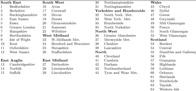
The 64 counties

South East South West 30 Northamptonshire Wales

1 Bedfordshire 16 Avon 31 Nottinghamshire 45 Clwyd

2 Berkshire 17 Cornwall Yorkshire and Humberside 46 Dyfed

3 Buckinghamshire 18 Devon 32 South York. Met. 47 Gwent

4 East Sussex 19 Dorset 33 West York. Met. 48 Gwynedd

5 Essex 20 Gloucestershire 34 Humberside 49 Mid Glamorgan

6 Greater London 21 Somerset 35 North Yorkshire 50 Powys

7 Hampshire 22 Wiltshire North West 51 South Glamorgan

8 Hertfordshire West Midland 36 Greater Manchester 52 West Glamorgan 9 Isle of Wight 23 W.Midlands Met. 37 Merseyside Met. Scotland

10 Kent 24 Hereford and Worcester 38 Cheshire 53 Borders

11 Oxfordshire 25 Shropshire 39 Lancashire 54 Central

12 West Sussex 26 Staordshire North 55 Dumfries and Galloway

40 Cleveland 56 Fife

East Anglia East Midland ^{41 Cumbria} 57 Grampian

13 Cambridgeshire 27 Derbyshire 42 Durham 58 Highlands

14 Norfolk 28 Leicestershire 43 Northumberland 59 Lothians

15 Suolk 29 Lincolnshire 44 Tyne and Wear Met. 60 Orkneys

61 Shetlands 62 Strathclyde 63 Tayside 64 Western Isle

Table 5: List of counties. Note: Surrey (South East) and Warwickshire (West Midlands) not included due to missing observations for some years.

Bandwidth selection for density estimation

Using the method of Sheater and Jones (1991), we have calculated the bandwidths reported in the table below.

81 82 83 84 85 86 87 88 89 90 91 92 93 94 95

h 0.22 0.20 0.16 0.17 0.20 0.19 0.20 0.24 0.26 0.22 0.17 0.12 0.11 0.14 0.15

Table 6: Bandwidth selected by Sheather and Jones (1991) plug{in method.

Bootstrap Multimodality Tests

A formal unimodality test is constructed based on the concept of critical bandwidth introduced by Silverman (1981, 1983, 1986). A critical bandwidth ^

h

m is dened as the smallest possible

h

producing a density with at most

m

modes, which means that for all

h <

^{^}

h

m the estimated density ^

f

h has at least

m

+ 1 modes. This idea of critical smoothing is naturally related to hypothesis testing and, in particular, to multimodality tests. Indeed, if the true underlying density has two modes, a large value of ^

h

1 is expected, because a

considerable amount of smoothing is required to obtain a unimodal density estimate from a bimodal density. This suggests that ^

h

m can be used as a statistic to test

H

0:

f

(

x

) has

m

modes versus

H

1:

f

(

x

) has more than

m

modes

:

(6) Here, a `large' value of ^

h

m indicates more than

m

modes, thus rejecting the null. How large is large in this context is assessed by the bootstrap, as discussed by Silverman and, among the others, by Izenman and Sommer (1988) and Efron and Tibshirani (1993).

The steps to test for multimodality can then be summarised as:

1. Draw

B

bootstrap samples

x

of size

n

using (5)

2. for each boostrap sample

x

compute the critical bandwidth consistent with

m

- modality, ^

h

_m. Denote the values of ^

h

_m by ^

h

_m(1)

^{^}

h

_m(2)

::: h

^{^}_m(

B

)

3. obtain an estimate of the achieved signicance level (or

p

-value) of the test as

ASL

^d m=

#^f^

h

_m(

b

) ^

h

m^g

=B

¹⁴

4. fail to reject the null hypothesis of

m

modes in the density whenever

ASL

^d m is larger than standard levels of signicance.

By implementing the above test in each year, we have obtained the results shown in Table 7. In all years, we fail to reject unimodality.

Year ASL (m = 1)^d ASL (m = 2)^d

1981 0.50 0.53

1982 0.20 0.63

1983 0.77 0.57

1984 0.52 0.24

1985 0.79 0.85

1986 0.76 0.31

1987 0.49 0.27

1988 0.79 0.47

1989 0.76 0.74

1990 0.60 0.98

1991 0.98 0.84

1992 0.92 0.63

1993 0.59 0.79

1994 0.88 0.49

1995 0.36 0.36

Table 7: Bootstrap multimodality tests with

B

= 1000 replications.

14It has been proven by Silverman that the event ^hm>^{^}hmis equivalent to the event that ^f^{^}_hm has more thanmmodes. This result implies that it is not necessary to compute ^hmfor each bootstrap sample one needs only to check the proportion of cases when ^f_h has more thanmmodes.

References

Barro, R. J. and Sala-i-Martin X. (1995), \Economic Growth", McGraw-Hill, New York.

Bianchi, M. (1995

a

), \Bandwidth selection in density estimation", in \The XploRe Book", Hardle W., Klinke S., and B.A. Turlach editors, Springer Verlag.

Bianchi, M. (1997), \Testing for convergence: Evidence from nonparametric multimodality tests", Journal of Applied Econometrics, 12, 393-409.

Bianchi, M. and G. Zoega (1996) \How quickly do British regions recover?", discussion paper no. 22/96, Birkbeck College.

Blackaby, D.H. and N. Manning (1981), \Applications of a Continuous Spatial Choice Logit Model", in C. Manski and D. McFadden, eds., Structural Analysis of Discrete Data with Econometric Applications, MIT Press.

Blanchard, Olivier J and Lawrence Katz (1992), \Regional Evolutions", Brookings Papers on Economic Activity, 1, 1-75.

Decressin, Jorg and Antonio Fatas (1995), \Regional Labour Market Dynamics in Europe", European Economic Review, 9, p. 1627-1657.

Efron, B. and R.J. Tibshirani (1993), An Introduction to the Bootstrap, Chapman and Hall, Monographs on Statistics and Applied Probability, 57, New York.

Evans, Philip and Barry McCormick (1994), \The New Pattern of Regional Unemployment:

Causes and Policy Signicance", The Economic Journal, 104, 633-647.

Hardle, W. (1990), Smoothing techniques with implementation in S, Springer-Verlag, Berlin.

Hughes, G. A. and Barry McCormick (1987), \Housing Markets, Unemployment and Labour Market Flexibility in the UK", European Economic Review , 31, 615-645.

Hughes, G. A. and Barry McCormick (1994), \Did Migration in the 1980s Narrow the North-South Divide?", Economica, 509-527.

Izenman, A.J. and C.J. Sommer (1988), \Philatelic mixtures and multimodal densitites", Journal of the American Statistical Association, 83 (404), 941-953.

Jackman, R. and S. Savouri (1992), \Regional Migration in Britain: An Analysis of Gross Flows using NHS Central Register Data", The Economic Journal, 102, 1433-1450.

Jimeno, Juan F. and Samuel Bentolila (1995), \Regional Unemployment Persistence (Spain, 1976-1994)", CEMFI Discussion Paper no. 95-09.

Marron, J.S., M.C. Jones and S. J. Sheather (1992), \Progress in data-based bandwidth selection for kernel density estimation", manuscript.

Pencavel, John (1994), \British Unemployment: Letter from America", The Economic Journal, 104, 621-632.

Pissarides, Christopher and Ian McMaster (1990), \Regional Migration, Wages, Unem- ployment: Empirical Evidence and Implications for Policy", Oxford Economic Papers, 42, 812-831.

Pissarides, Christopher and Jonathan Wadsworth (1989), \Unemployment and the Inter- Regional Mobility of Labour", The Economic Journal, 99, 739-755.

Sheather, S.J. and M.C. Jones (1991), \A reliable data-based bandwidth selection method for kernel density estimation", Journal of the Royal Statistical Society, 26, Series B, 683- 690.

Silverman, B.W. (1986), Density estimation for statistics and data analysis, Chapman and Hall, Monographs on statistics and applied probability no. 26, London.

Silverman, B.W. (1981), \Using kernel density estimates to investigate multimodality", Journal of the Royal Statistical Society, Series B, 43, 97{99.

Silverman, B.W. (1983), \Some properties of a test for multimodality based on kernel density estimates", in Probability, Statistics, and Analysis. Edited by J.F.C. Kingman and G.E.H. Reuter, Cambridge University Press, 248{260.