Characteristics of Unemployment Dynamics: The Chain Reaction Approach

IHS Economics Series Working Paper 205

April 2007

Characteristics of Unemployment Dynamics: The Chain Reaction Approach

Marika Karanassou

Dennis J. Snower

Impressum Author(s):

Marika Karanassou, Dennis J. Snower Title:

Characteristics of Unemployment Dynamics: The Chain Reaction Approach ISSN: Unspecified

2007 Institut für Höhere Studien - Institute for Advanced Studies (IHS) Josefstädter Straße 39, A-1080 Wien

E-Mail: o ce@ihs.ac.atffi Web: ww w .ihs.ac. a t

All IHS Working Papers are available online: http://irihs. ihs. ac.at/view/ihs_series/

This paper is available for download without charge at:

https://irihs.ihs.ac.at/id/eprint/1765/

205 Reihe Ökonomie Economics Series

Characteristics of Unemployment Dynamics:

The Chain Reaction Approach

Marika Karanassou, Dennis J. Snower

205 Reihe Ökonomie Economics Series

Characteristics of Unemployment Dynamics:

The Chain Reaction Approach

Marika Karanassou, Dennis J. Snower April 2007

Institut für Höhere Studien (IHS), Wien

Contact:

Marika Karanassou Department of Economics Queen Mary and Westfield College Mile End Road

London E1 4NS, United Kingdom email: m.karanassou@qmul.ac.uk Dennis J. Snower

The Kiel Institute for the World Economy Düsternbrooker Weg 120

24105 Kiel, Germany : +49/431/8814-235

email: dennis.snower@ifw-kiel.de

Founded in 1963 by two prominent Austrians living in exile – the sociologist Paul F. Lazarsfeld and the economist Oskar Morgenstern – with the financial support from the Ford Foundation, the Austrian Federal Ministry of Education and the City of Vienna, the Institute for Advanced Studies (IHS) is the first institution for postgraduate education and research in economics and the social sciences in Austria.

The Economics Series presents research done at the Department of Economics and Finance and aims to share “work in progress” in a timely way before formal publication. As usual, authors bear full responsibility for the content of their contributions.

Das Institut für Höhere Studien (IHS) wurde im Jahr 1963 von zwei prominenten Exilösterreichern – dem Soziologen Paul F. Lazarsfeld und dem Ökonomen Oskar Morgenstern – mit Hilfe der Ford- Stiftung, des Österreichischen Bundesministeriums für Unterricht und der Stadt Wien gegründet und ist somit die erste nachuniversitäre Lehr- und Forschungsstätte für die Sozial- und Wirtschafts- wissenschaften in Österreich. Die Reihe Ökonomie bietet Einblick in die Forschungsarbeit der Abteilung für Ökonomie und Finanzwirtschaft und verfolgt das Ziel, abteilungsinterne Diskussionsbeiträge einer breiteren fachinternen Öffentlichkeit zugänglich zu machen. Die inhaltliche Verantwortung für die veröffentlichten Beiträge liegt bei den Autoren und Autorinnen.

Abstract

The aim of this paper is to analyze and estimate salient characteristics of unemployment dynamics. Movements in unemployment are viewed as "chain reactions" of responses to labour market shocks, working their way through systems of interacting lagged adjustment processes. In the context of estimated labour market systems for Germany, the UK, and the US, we construct aggregate measures of unemployment responses to temporary and permanent shocks. These measures are temporal and quantitative. Furthermore, we estimate the contributions of individual lagged adjustments to these aggregate measures.

Our empirical results indicate that lagged adjustment processes play an important part in explaining how temporary and permanent shocks affect unemployment, that temporary and permanent shocks can yield quite different inter-country comparisons of unemployment effects, and that the quantitative and temporal measures can also yield markedly different inter-country comparisons.

Keywords

Unemployment, natural rate hypothesis, labour markets, employment, adjustment costs

JEL Classification

J32, J60, J64, E30, E37

Comments

We gratefully acknowledge the financial support by the Jubilaeumsfonds of the Austrian National Bank Grant no. 10088, from IZA, and the Leverhulme Grant on Unemployment Dynamics and Matching

Contents

1 Introduction 1

2 A Model of Unemployment Persistence and

Responsiveness 4

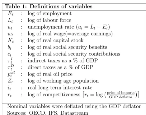
2.1 The Underlying Model ... 4

2.2 Unemployment Persistence ... 9

2.2.1 Quantitative and Temporal Persistence ... 10

2.2.2 Sources of Unemployment Persistence ... 11

2.3 Imperfect Unemployment Responsiveness ... 13

2.3.1 Quantitative and Temporal Responsiveness ... 13

2.3.2 Sources of Imperfect Responsiveness ... 15

2.4 The Relation between Persistence and Imperfect Responsiveness ... 15

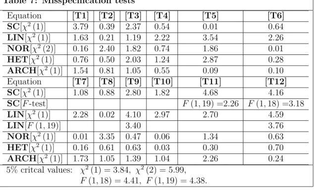
3 Empirical Analysis 18

3.2 Estimating Persistence and Imperfect Responsiveness ... 20

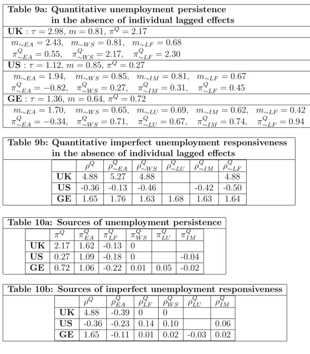
3.2.1 Deriving the Measures of Persistence and Imperfect Responsiveness ... 20

3.2.2 Empirical Results on Aggregate Persistence ... 21

3.2.3 Empirical Results on Imperfect Responsiveness ... 22

3.3 Estimating the Sources of Persistence and Imperfect Responsiveness ... 23

4 Concluding Thoughts 25

References 28 Tables 30

Appendix 1 35

Appendix 2 40

Appendix 3 44

1 Introduction

Much of the existing unemployment literature draws on two alternative, ex- treme views of how unemployment moves through time: the natural rate and hysteresis theories. The natural rate theory, in its simplest form, represents unemployment movements as random variations around a reasonably sta- ble natural rate of unemployment; and in more sophisticated developments,

the natural rate is portrayed as moving in response to permanent shocks in the stationary, long-run equilibrium unemployment rate (e.g. changes in unemployment benefits, taxes, social security contributions, interest rates, and union density). The hysteresis theory, by contrast, asserts that unem- ployment tends to get stuck at wherever the previous labour market shocks have placed it. In the former view temporary labour market shocks have temporary unemployment effects; whereas in the latter view these shocks lead to permanent changes in unemployment.

Numerous studies attempt to bridge the gap between these extreme positions; they do so by suppos- ing that unemployment depends on its lagged values but tends towards a stable natural rate, as in the dynamically stable variants of the equation

u

= P

i=1

α

u

+ βx

+ ε

, ε

∼ i.i.d (0, σ

). Then the natural rate is u

=

i=1αi

. In such hybrid models, temporary labour market shocks (ε

) have persistent, but not permanent, effects on unemployment.

All the above approaches, however, tend ignore two interesting and po- tentially important dimensions of the unemployment problem:

1. Not only are current labour market decisions - such as employment, wage setting, and labour force participation decisions - characterised by lagged responses to past labour market activities,

but these lagged responses interact with one another in affecting unemployment. If the lagged responses are complementary to one another, it will take unem- ployment much longer to recover in the aftermath of a recession than the period spanned by any particular lag. For example, a current drop in labour demand can depress employment in the following period on

1See, for example, Phelps (1994).

2The simplest representation of the natural rate theory is ut = uⁿ+εt, where ut is the unemployment rate at time t, uⁿ is the natural rate, and εt is a strict white noise stochastic process. An analogous representation of the hysteresis theory isut=u_t−1+εt.

3The coefficientsαi are constants,βxtis a linear combination of exogenous variables, and the roots of the characteristic equationλ^p−α1λ^p−1−...−αp= 0 lie inside the unit circle, so that the equation is dynamically stable.

4For instance, firms’ current employment decisions commonly may depend on their past employment on account of labour turnover costs, and current wage decisions depend on past unemployment when search effort declines with people’s duration of unemployment.

account of labour turnover costs; this raises the duration of people’s unemployment spells, thereby reducing search intensity and depress- ing employment in the next period; and so on. Thus, unemployment movements that are commonly attributed to changes in the NAIRU or to hysteretic responses to temporary shocks may arise from a lengthy interaction among various lagged adjustment processes. This point is obvious, but the interaction of lagged adjustment processes has received little explicit attention in the unemployment literature thus far.

2. Furthermore the resulting network of lagged labour market adjustment processes interacts with the dynamic structure of the labour market shocks. Naturally, unemployment responds differently through time to a temporary shock than to a permanent one. In the context of a first-order unemployment autoregression it is well-known, for example, that the more long-lasting are the unemployment effects of a temporary shock, the longer it takes for unemployment to approach its long-run equilibrium in response to a permanent shock; in short, the degree of unemployment persistence in response to temporary shocks is posi- tively related to the degree of inertia in response to permanent shocks.

But for higher-order unemployment autoregressions, this correspon- dence breaks down: unemployment persistence may be positively or negatively related to unemployment inertia. Thus far little has been done to provide theoretical and empirical analyses of how lags in labour demand, wage setting, and labour force participation schedules influ- ence the relation between the unemployment effects of temporary and permanent shocks.

The natural rate theory underplays the first dimension - the interactions among lagged labour market adjustment processes - by focusing attention on the long-run equilibrium unemployment rate that is reached once the adjust- ment processes have worked themselves out. The hysteresis theory avoids ex- amining the lagged interactions by focusing on the unit root of the time-series unemployment process.

The hybrid models above, based on single-equation models of unemployment, do not do justice to the lagged interactions either.

The empirical single-equation models are meant to be summaries of empir- ical multi-equation labour market systems,

but the lagged interactions in

5In general, there is of course no reason why the lagged interactions should imply a unit root; this could happen only by accident.

6In the systems approach unemployment is typically portrayed as the difference between labour supply and labour demand in a system containing employment, wage setting, and labour force participation equations.

the empirical systems do not aggregate to produce equivalent unemployment dynamics in the empirical single-equation models.

In particular, the statis- tically significant lags in the single-equation models characteristically imply far less unemployment persistence (in response to temporary shocks) than is implied by the statistically significant lags of estimated multi-equation labour market systems.

Many of the conventional unemployment models overlook the second dimension above, since they focus primarily on temporary labour market shocks. The random variations around the natural rate are temporary; so are the shocks that lead to the permanent unemployment effects in the hysteresis models and to the long-lasting unemployment effects in the hybrid models above. But in practice labour market shocks have both temporary and per- manent components. Whereas some aggregate business cycle fluctuations are temporary, changes in productivity, exchange rates, raw material prices, taxes, and real interest rates are often permanent. The interplay between shock dynamics and labour market dynamics requires explicit attention.

The aim of this paper is to focus on the neglected dimensions above.

We will consider labour market models where current decisions - regarding employment, wage setting, and labour force participation - depend on past decisions, and where these lagged adjustments interact. These interactions are the centerpiece of the chain reaction theory of unemployment, in which each labour market shock has a “chain reaction” of unemployment effects.

The network of lagged adjustment processes is the propagation mechanism for this chain reaction.

In this context, we will construct aggregative summary measures of the dynamic unemployment responses to temporary and permanent shocks. We will be concerned with two important dynamic influences: (i) the persistent unemployment effects of temporary shocks, called unemployment persistence, and (ii) the delayed unemployment effects of permanent shocks, which we will call imperfect unemployment responsiveness. Our aggregative measures of unemployment persistence and imperfect unemployment responsiveness can perform a useful role in characterising the movement of unemployment through time, analogous to the way in which macroeconomic indices (such as GNP or inflation) are useful in characterising macroeconomic activity at each point in time.

Focusing on three countries - Germany, the United Kingdom, and the United States - we will identify significant lags in labour demand, wage set- ting, and labour force participation behaviour, and measure the degree to

7The econometric reasons for this failure are well-known, e.g. nonlinearities in t- statistics.

which these lags are responsible for unemployment persistence and imperfect responsiveness. Elsewhere it has been shown that lagged unemployment re- sponses to temporary and persistent shocks - as captured through unemploy- ment persistence and imperfect responsiveness - play an important role deter- mining the evolution of unemployment in various industrialised economies.

Our analysis of the sources underlying persistence and responsiveness con- stitutes a first step toward providing an understanding the medium- and longer-term movements of unemployment.

The policy implications of our approach are striking. First, since differ- ent employment policies affect different lagged adjustments, examining the role of each lag within its network of lagged adjustments is important for policy formulation. Second, labour market shocks of different durations may require different policy responses. And finally, since lagged labour market ad- justment processes tend to differ markedly from country to country, different countries may require different policies to deal with what looks superficially as a similar unemployment problem.

The rest of the paper is organised as follows. Section 2 presents a theo- retical model of unemployment persistence and responsiveness and analyzes how the lagged adjustment processes contribute to these phenomena. Section 3 contains our empirical analysis, in which we examine how the movement of unemployment in Germany, the UK, and the US over the past four decades can be clarified through the concepts above. Finally Section 4 concludes.

2 A Model of Unemployment Persistence and Responsiveness

The theoretical model in this section provides a background for the empir- ical model of Section 3. In particular, the theoretical model illustrates how the interaction among lagged labour market adjustment processes generates persistence and imperfect responsiveness of unemployment. It indicates how these two phenomena are distinct from one another, describing different dy- namic features of unemployment. These features, together, will provide in- sights into the way unemployment moves through time.

2.1 The Underlying Model

Our theoretical framework provides simple examples of lagged adjustment processes occurring in labour demand, wage setting, and labour force partic-

8See, for example, Karanassou and Snower (1998, 2000).

ipation decisions.

We consider a labour market containing a fixed number of identical firms with monopoly power in the product market. The i’th firm has a production function of the form

q

= Ae

k

, (1a) where q

is output supplied, e

is employment, k

is capital stock, A, α, β are positive constants, and 0 < α < 1. Each firm faces a product demand function of the form

q

= p

p

y

f , (1b)

where y

stands for aggregate product demand, f is the number of firms, p

is the price charged by firm i, p

is the aggregate price level, and η is the price elasticity of product demand (a positive constant). Note that the firms are assumed to face symmetric production and cost conditions.

To derive the firm’s labour demand function, we observe that the firm sets its employment at the profit maximizing level, at which the marginal revenue from producing an extra unit of output is equal to the corresponding marginal cost (for a given capital stock). The marginal revenue is M R

= p

1 −

. Let the marginal cost be M C

= ω

i,t

∂qi,t

ξ

, where ω

is the wage paid by the firm,

i,t

is the marginal labour requirement, and ξ

is an employment adjustment parameter. The employment adjustment parameter is ξ

= (e

/σe

)

, where δ is a positive constant and σ is the

“survival rate,” i.e. one minus the separation rate. For simplicity, we assume that the separation rate is sufficiently high (the survival rate is sufficiently low), so that e

> σe

. The employment adjustment parameter may be interpreted in terms of training costs: e

/σe

= 1 + (h

/σe

), where h

is new hires. The training of new hires (h

) in period t is done by the incumbent employees (σe

) in that period. The greater the ratio of new hires to incumbent employees, the greater the average training cost per employee (ξ

). When δ = 0 (so that ξ

= 1), the employment adjustment cost is zero; and when δ > 0 (so that ξ

> 1), the adjustment cost is positive.

For the production function above, the marginal product of labour (the inverse of the marginal labour requirement) is

i,t

= αAe

k

. Thus the marginal cost is M C

=

e

k

ξ

. Setting the marginal revenue equal

9Our analysis is in the spirit of recent theoretical models of aggregate labour market activity (e.g. Layard, Nickell and Jackman (1991), Lindbeck and Snower (1989), Nickell (1995)).

to the marginal cost, we obtain the firm’s (implicit) labour demand function:

ω

αA e

k

e

σe

= p

1 − 1 η

. (2)

In the labour market equilibrium, p

= p

and ω

= ω

, due to sym- metry. Aggregating the individual firms’ labour demand functions, taking logarithms, so that E

= log (f e

) K

= log (f k

), and introducing an error term (ε

) to capture technological shocks, we obtain the following aggregate employment equation:

E

= a

+ a

E

− a

w

+ a

K

+ ε

, (3) where w

= log (ω

/p

) and ε

∼ i.i.d (0, σ

). The parameter a

will be called the “employment inertia coefficient.” When the employment adjustment cost is zero (δ = 0), the employment inertia coefficient is zero; when the adjustment cost is positive (δ > 0), the employment inertia coefficient is positive as well.

For simplicity, let the wage be equal to the reservation wage of the marginal employee. Suppose that the population of workers is heteroge- neous in terms of the disutility of work and thus also in terms of the reser- vation wage. Moreover, suppose that this population can be ordered along a reservation wage continuum, from lowest to highest, so that when aggre- gate employment rises, the reservation of the marginal worker rises as well.

Assuming this relation to be linear, our wage setting equation becomes

w

= b + b

E

. (4)

The labour force participation decision equates the marginal return from being in the labour force with the associated marginal cost being in the labour force. For simplicity, let the per capita return (in logs) from being in the labour force be positively related to the employment probability (E

− L

, where L

is the size of the labour force, in logs) and to the wage (w

), and negatively related to the inactivity rate (L

−Z

, where Z

is the log of working age population). Specifically, let the return from being in the labour force be given by d

+ d

(E

− L

) + d

w

− d

(L

− Z

), where d

, d

, d

and d

are positive constants.

Regarding the cost per capita of being in the labour force, suppose that there are costs of entry into the labour force and that these costs depend

10a^∗ = ^log(1−¹_η)^{+log(αA)+δlog}σ+(1−α−β) logf

1+δ−α , and a^∗_E = _1+δ−α^δ , andaw = _1+δ−α¹ , a^∗_K =

β 1+δ−α.

positively on the ratio of new labour force entrants to incumbent members of the labour force. Accordingly, let the cost per capita (in logs) be given by c

+ c

L

− c

L

(where the new labour force entrants are positively related to L

− L

, the number of incumbents are positively related to L

, and c

> c

). Setting the per capita return equal to the per capita marginal cost, we obtain the following labour force participation equation:

L

= c

+ c

L

+ c

w

+ c

E

+ c

Z

, (5) The coefficient c

may be called the “labour force inertia coefficient.”

Substitution of equation (4) into (3) and (5) yields:

E

= a + a

E

+ a

K

+

1 1 + a

b

ε

, (6)

L

= c + c

L

+ c

E

+ c

Z

, (7) where a =

wbE

, a

=

wbE

, a

=

wbE

, c = c

+ c

b, c

= c

+ c

b

. (Note that 0 < a

< 1, and 0 < c

< 1.)

Finally, the unemployment rate u

may be approximated as the difference between the log of the labour force L

and the log of employment E

:

u

= L

− E

. (8)

The model contains two lagged adjustment effects: (i) current employ- ment depends on past employment, (ii) the current labour force depends on the past labour force. For ease of exposition, we will call these two effects the employment adjustment effect,

and the labour force adjustment effect, respectively. It is important to emphasize that these names are merely heuris- tic devices that help us refer the individual lagged effect.

The employment adjustment, and labour force adjustment effects are usually taken to be pos- itive: a

, c

> 0 and we will maintain this assumption here.

11c^∗=_c^−c1+d1

2+d₂+d₄,cw= _c ^d3

2+d₂+d₄,c^∗_E= _c ^d2

2+d₂+d₄,cL=_c ^c3

2+d₂+d₄,andcZ = _c ^d4

2+d₂+d₄.

12For instance, firms’ current employment decisions commonly may depend on their past employment on account of costs of labour turnover costs (e.g. Lindbeck and Snower (1988) and Nickell (1978)).

13We naturally do not wish to imply that the employment adjustment effect arises only account of employment adjustment costs, and that the labour force adjustment effect arises only account of labour force adjustment costs . Clearly, when agents optimise their objectives intertemporally, each of the individual lagged effects will, in general, arise from a variety of sources.

Equations (6)-(8) yield the following reduced form unemployment rate equation:

u

= (a

+ c

) u

− a

c

u

−

1 − c

1 + a

b

ε

+

c

1 + a

b

ε

− a

(1 − c

) K

+ a

c

K

+ac

+ (1 − a

) c − (1 − c

) a + c

Z

− c

a

Z

. (9) As noted, the labour market system (6)-(8) is merely illustrative of in- teracting lagged adjustment processes in the labour market. The micro- foundations of these and other lagged adjustments have been explored ex- tensively in the theoretical literature.

Whereas the equations above have been derived in particularly simple ways, in general these equations are the outcomes of complex intertemporal optimisation problems. For instance, a labour demand equation is usually derived from the maximisation of the firms’ present value of profits (under perfect or imperfect competition) sub- ject to sequences of production function constraints; a wage setting equation is generally be derived on the basis of bargaining between firms and their employees, efficiency wage setting by firms, or labour union wage setting;

and a labour force participation equation is often derived from workers’ in- tertemporal utility maximisation subject to sequences of budget constraints.

In these intertemporal contexts, employment, wage, and labour supply de- cisions depend on the agents’ rational expectations of future economic vari- ables. These expectations may be expressed in terms of the present and past values of these economic variables, which are then substituted into the rel- evant first-order conditions of agents’ optimisation problems. Consequently, the labour demand, wage setting, and labour force participation equations may be expressed in terms of present and past variables, as illustrate in the model above.

The focus of attention in this paper is not, however, the microeconomic sources of the lagged labour market adjustments; rather, we are interested in how these lagged adjustments (whatever their sources) interact with one another and with labour market shocks to generate an unemployment tra- jectory. For this purpose, we suppose that the participants in the labour market face known distributions of labour market shocks. These shocks may take the form of white noise variations in the labour demand, wage setting,

14See Appendix 1, eq.(A1.4) and (A1.4’).

15For example, Taylor (1979) rationalise the dependence of current wages on past wages, Lindbeck and Snower (1987) rationalise the relation between current wages and past em- ployment, and so on.

and labour supply equations (that are temporary shocks) and variations in the future realizations of the exogenous variables (that could be permanent shocks).

On this basis, they make their labour market decisions, yielding an equation system with lagged adjustments (such as the illustrative one above), which we take as the starting point of our analysis. We then con- sider how realizations of the temporary and permanent shocks interact with the system’s network of lagged adjustments to generate unemployment per- sistence and imperfect unemployment responsiveness. It is this interaction that occupies centre-stage in our analysis.

With this in mind, we now examine how temporary and permanent shocks give rise to chain reactions of unemployment effects.

2.2 Unemployment Persistence

Suppose that in period t there is a temporary (one-period) unit fall in labour demand: dε

= −1. The immediate impact is of course to reduce employment and thereby raise unemployment by a unit. Thereafter (in periods t+i, i > 0) the labour demand shock dε

has the following two effects.

• (i) Via the employment adjustment effect (whose magnitude is given by the coefficient a

), the shock dε

reduces employment E

(by a

dε

) below what it would have been in the absence of the shock (and thus raises unemployment u

).

• (ii) Via the labour force adjustment effect (whose magnitude is given by the coefficient c

), the shock reduces the labour force L

(by c

dε

) below what it would otherwise have been (and thereby reducing unem- ployment u

).

The movement of unemployment in response to the temporary shock may be explained wholly through the interactions of these three effects.

It can be shown that the unemployment response j periods after the shock is

du

= a

[(1 − c

) a

− c

] + c

c

(1 + a

b

) (a

− c

) , (10)

16An example is capital stock in the model above.

17It is important that the shocks be realizations from the known distributions generating the error terms and exogenous variables, for otherwise the occurrence of a new shock may be expected to affect the agents’ decision making, leading to revised employment, wage setting, and labour supply equations (with revised lag structures).

18The chain reaction of unemployment movements, period by period, is described in Appendix 1.

where du

is the difference between unemployment in the presence and absence of the shock.

This indicates how the unemployment effects of the temporary shock persist through time.

2.2.1 Quantitative and Temporal Persistence

The phenomenon of “unemployment persistence” has two interesting fea- tures, which may be measured by two separate statistics:

(1) Quantitative unemployment persistence measures the degree to which unemployment is affected by the temporary shock after that shock has dis- appeared. Specifically, for a unit shock occurring in period t, it is the sum of the unemployment effects for all periods t + j, j ≥ 1:

π

=

∞

X

j=1

du

. (11a)

In the absence of lagged labour market adjustment processes, unemployment would not be affected after the temporary shock has disappeared and thus quantitative unemployment persistence π

would be zero. At the opposite extreme of hysteresis, the temporary shock would have a permanent effect on unemployment and thus π

would be infinite.

(2) Temporal unemployment persistence measures how long it takes for the unemployment effect of the shock to shrink to a fraction κ of its initial value. Specifically, it measures the maximum number of periods, after the occurrence of the unit shock, over which the unemployment effect exceeds the fraction κ of the initial effect:

π

= arg max

j>0

(|du

| > κ |du

|) . (11b) Once again, in the absence of lagged adjustment processes, π

would be zero;

whereas in the presence of hysteresis, π

would be infinite.

The two statistics are concerned with different economic phenomena.

Whereas quantitative persistence is concerned with the cumulative amount of unused labour resources over time generated in the aftermath of the tempo- rary shock, temporal persistence deals with the time required for the influence of the shock to disappear.

19Thus the operator d describes a comparative static difference (rather than a change through time).

20In other words, temporal persistence measures how long it takes for unemployment to return to a specified neighbourhood of the time path it would have followed in the absence of the shock.

For the unemployment equation (9), the degree of quantitative unemploy- ment persistence is

:

π

= a

(1 − c

) (1 − c

) − c

c

(1 + a

b

) (1 − a

) (1 − c

) , (12) whereas the degree of temporal unemployment persistence cannot be derived explicitly in general terms.

2.2.2 Sources of Unemployment Persistence

With a view to the empirical analysis later, we examine the sources of un- employment persistence by showing how each of the lagged adjustment pro- cesses contributes to unemployment persistence. For brevity, we focus on quantitative persistence π

.

To measure the influence of the employment adjustment effect (EA) on quantitative persistence, we compute the difference between π

in the pres- ence and absence of the EA effect, given that the labour force adjustment effect is in operation. In the absence of the employment adjustment effect, the employment equation (3) becomes E

= a

+ a

E

− a

w

+ a

K

+ ε

. It can be shown

that the associated degree of persistence is

π

= −c

c

(1 + a

b

) (1 − a

) (1 − c

) < 0,

where “∼ EA” stands for the “absence of the employment adjustment effect.”

Thus our measure of the degree of quantitative unemployment persistence attributable to the employment adjustment effect is total persistence minus persistence in the absence of the EA effect:

π

= π

− π

= a

(1 − c

)

(1 + a

b

) (1 − a

) . (13a)

21See Appendix 1.

22The derivation of this and other sources of persistence is given in Appendix 1.

23Note that the influence of the employment adjustment effect on quantitative persis- tence cannot be measured by taking the derivative ofπ^Qwith respect toa_E, since a change inaEalters not only the magnitude of the employment adjustment process towards a given labour market equilibrium, but also alters the equilibrium itself. After all, unemployment persistence is about protracted adjustment to equilibrium rather than a shift of the equi- librium. To measure the contribution of a small change in the adjustment process on persistence, it would be necessary to specify the coefficients of the lagged variables in our labour market system in such a way that coefficient changes would leave the labour market equilibrium unchanged.

Similarly, the influence of the labour force adjustment effect on quantita- tive persistence may be evaluated by computing the difference between persis- tence in the presence and absence of this effect, in the presence of the employ- ment adjustment process. In the absence of the labour force adjustment ef- fect, the labour force equation (5) becomes L

= c

+c

L

+c

w

+c

E

+c

Z

and the associated degree of persistence is

π

= a

(1 − c

− c

)

(1 + a

b

) (1 − a

) (1 − c

) .

Hence the degree of quantitative unemployment persistence attributable to the labour force adjustment effect is

π

= π

− π

= −c

c

(1 + a

b

) (1 − c

) < 0. (13b) It is interesting to observe that the role of the adjustment processes is to determine how the unemployment effects of a temporary shock are split between the present and the future. To see this, let m (the “m ultiplier”) stand for the current effect of the shock on unemployment; f stand for the sum of the future effects; and τ = m + f stand for the total effect (over the present and future). For the labour market system (6)-(8),

m ≡ du

= 1 − c

1 + a

b

; f ≡ π

; τ = (1 − c

− c

)

(1 + a

b

) (1 − a

) (1 − c

) . (14a) However, in the absence of the employment adjustment effect:

m

= 1 − c

(1 + a

b

) (1 − a

) ; f

= π

; m

+ f

= τ; (14b) and in the absence of the labour force adjustment effect:

m

= 1 − c

− c

(1 + a

b

) (1 − c

) ; f

= π

; m

+ f

= τ . (14c) Equations (14a-c) show that the presence of the lagged adjustment processes influences the distribution of unemployment effects through time (the relative magnitude of m and τ , the current and future effects), but not the total effect τ .

Finally, observe that adding the sources of persistence (π

+ π

) does not yield the aggregate measure of persistence (π

). The reason of course is that each source of persistence is measured by taking the difference be- tween persistence in the presence and absence of that sources, assuming that the other source is operative. Since the different sources interact with one another, the various sources cannot be added to yield aggregate persistence.

24In fact, it can be shown thatπ^Q_EA+π^Q_LF > π^Q,i.e. the employment and labour force

2.3 Imperfect Unemployment Responsiveness

Next consider the chain reaction of unemployment changes in response to a permanent labour demand shock. Assuming that the capital stock follows a random walk, K

= K

+ v

, we let the permanent shock be represented by a realization of the white noise error term v

in this stochastic process.

Specifically, suppose that in period t there is a temporary (one-period) unit fall in v

, which has a permanent negative influence on the capital stock K

. In the initial period t, the employment effect of this fall in the capital stock is dE

= −a

. In subsequent periods the shock has the following effects:

(i) it continues to have a direct effect on employment by dE

= −a

in each period j > 0 (since the influence on the capital stock is permanent);

(ii) due to the employment adjustment effect, the fall in employment E

reduces employment E

below what it would have been in the absence of the shock; and (iii) due to the labour force adjustment effect, the fall in employment E

reduces the labour force L

below what it would otherwise have been.

These three effects all interact with one another, producing a chain re- action of unemployment movements, so that the unemployment response j periods after the period-t shock is

du

=

a

a

− c

"

(1 − c

)

j

X

i=0

a

− c

− c

j

X

i=0

a

− c

#

, (15) where du

is now defined as the difference between unemployment in the presence and absence of the permanent labour demand shock.

2.3.1 Quantitative and Temporal Responsiveness

Analogously to our analysis of unemployment persistence, we assess imperfect unemployment responsiveness from two vantage points:

(1) Quantitative imperfect responsiveness measures the cumulative unem- ployment effect of the permanent shock that arises because unemployment does not adjust immediately to the new long-run equilibrium. In particular, for a unit shock beginning in period t, quantitative imperfect responsiveness is the sum of the differences through time between (a) the disparity between

adjustment effects are substitutes in this model (i.e. the joint effects are less than the sum of the individual effects).

25For simplicity, we also assume that the error termsεt andvt are independent of one another.

26The theoretical results on imperfect responsiveness are derived in Appendix 2.

actual and long-run unemployment in the presence of the shock and (b) this disparity in the absence of the shock:

ρ

=

∞

X

j=0

(du

− du

) . (16a)

By equation (15), the effect of the permanent shock on long-run employment is

du

≡ lim

j→∞

du

= a

(1 − c

− c

) (1 − a

) (1 − c

) .

In the absence of lagged labour market adjustment processes, unemploy- ment would be “perfectly responsive,” i.e. it would adjust immediately to its new long-run expected rate, and thus ρ

would be zero. If however the full effects of the permanent labour demand shock emerge only gradually, so that the short-run unemployment effects of the shock are less than the long-run effect, then unemployment is “under-responsive”: ρ

< 0, i.e. unemploy- ment displays inertia. On the other hand, if unemployment overshoots its long-run equilibrium, then our measure may be positive, making unemploy- ment “over-responsive”: ρ

> 0. As we approach hysteresis, ρ

approaches infinity.

For the unemployment rate equation (9), the degree of quantitative im- perfect unemployment responsiveness may be derived explicitly:

ρ

= a

[−a

(1 − c

− c

) (1 − c

) + c

c

(1 − a

)]

[(1 − a

) (1 − c

)]

. (17) (2) Temporal imperfect responsiveness measures how long its takes for unemployment to reach a particular neighbourhood of its new long-run equi- librium. Specifically, it measures the maximum number of periods j over which the difference du

− du

(i.e. the difference between the actual and long-run expected unemployment rates in the presence and absence of the shock in any period t + j) exceeds the fraction κ of the initial difference du

− du

:

ρ

= arg max

j>0

(|du

− du

| > κ |du

− du

|) . (16b) As above, ρ

would be zero in the absence of labour market lags, and it approaches infinity as we approach hysteresis.

27This is equivalent to the differences through time between (a) the disparity between the actual unemployment rate in the presence and absence of the shock (dut+j), and (b) the disparity between the long-run unemployment rate in the presence and absence of the shock (du^∗).

28See Appendix 2.

2.3.2 Sources of Imperfect Responsiveness

We now turn to the sources of imperfect responsiveness. In the absence of the employment adjustment effect, it can be shown that the degree of imperfect responsiveness is

ρ

= a

c

c

(1 − a

) (1 − c

)

> 0.

If c

+ c

< 1 then ρ

> ρ

, i.e. the employment adjustment effect magnifies the inertia of unemployment, making unemployment to respond more slowly to a permanent labour demand shock than it would otherwise have done.

Thus the degree of quantitative responsiveness attributable to the employment adjustment effect is

ρ

= ρ

− ρ

= − a

a

(1 − c

− c

)

(1 − a

)

(1 − c

) , (18a) which is negative if c

+ c

< 1, i.e. the employment adjustment effect makes unemployment more under-responsive than it would otherwise have been (ρ

< 0).

Along the same lines, the degree of quantitative responsiveness attributable to the labour force adjustment effect is

ρ

= a

c

c

(1 − a

) (1 − c

)

> 0. (18b) Since the labour force adjustment effect causes the labour force to fall in the future (when c

> 0), in tandem with the fall in employment, this effect thereby reduces the inertia of unemployment, making unemployment less under-responsive that it would otherwise have been (ρ

> 0).

Observe that in this model there are no complementarities or substi- tutabilities between the two adjustment effects since ρ

+ ρ

= ρ

.

2.4 The Relation between Persistence and Imperfect Responsiveness

Persistence and imperfect responsiveness are the outcome of the same con- stellation of lagged labour market adjustment processes; the only difference

29See Appendix 2.

30In other words, unemployment is more over-responsive in the absence of the employ- ment adjustment effect than in its presence.

31This result is specific to our model. In other models, of course, sources of imperfect responsiveness may be complements or substitutes, in the sense that the joint effects may be greater or less than the sum of the individual effects, respectively.

between these phenomena lies in the nature of the labour market shock ini- tiating these processes. By exploring the relation between persistence and imperfect responsiveness, we can gain insight into how the interaction be- tween the shocks and the adjustment processes depends on the durability of the shocks.

The simplest - and, unfortunately, the most misleading - way of thinking about the relation between persistence and imperfect responsiveness is in the context of a first-order difference equation in unemployment. For instance, in our model above, suppose that there were no labour force adjustment effect (c

= 0). Thus the only remaining adjustment process is the employment adjustment effect (a

> 0). The unemployment equation (9’) then reduces to

u

= a

u

−

1 − c

1 + a

b

ε

+ −a

(1 − c

) K

+ac

+ (1 − a

) c + c

Z

− c

a

Z

,

In this simple context, it is easy to see that quantitative persistence and quan- titative imperfect responsiveness are inversely related to one another. Both depend on the magnitude of the autoregressive coefficient (a

). The greater is this coefficient, the greater is quantitative persistence

π

=

E)(1+awbE)

and the smaller is quantitative imperfect responsiveness

ρ

= −

E)²

. In other words, the greater is the autoregressive coefficient, the greater is the sum of the unemployment after-effects from a temporary shock and the smaller the sum of the unemployment responses to a permanent shock. Since persistence and imperfect responsiveness are tied to one another in this way, it is clearly unnecessary to view them as separate phenomena.

However, as noted, this account of the relation between persistence and imperfect responsiveness is misleading, since it invariably occurs only in first- order unemployment equations. For higher-order equations - the sort we are overwhelmingly likely to encounter in empirical labour market systems, where a variety of lagged adjustment processes are operative - the above relation is only one of various possibilities. Then, of course, persistence and imperfect responsiveness are indeed separate phenomena. Reintroducing the labour force adjustment effect into our model indicates why this is so.

In this expanded model (containing an employment adjustment effect

(a

> 0) and a labour force adjustment effect (c

> 0)), it turns out that,

when c

+c

< 1, the relation between persistence and imperfect responsive-

ness depends critically on the autoregressive coefficient a

, measuring the

employment adjustment effect. There are three scenarios:

1. When the employment adjustment effect is “high,” a

>

L)(1−c_E−c_L)+cEcL

, then quantitative persistence is positive π

> 0

and quantitative im- perfect responsiveness is negative ρ

< 0 (viz., “under-responsiveness”

to permanent shocks). This scenario exhibits inertia in response to both temporary and permanent shocks: (a) an unemployment-increasing temporary shock leads cumulatively to more unemployment after the shock has disappeared; whereas (b) an unemployment-increasing per- manent shock leads cumulatively to less unemployment than would have occurred under instantaneous adjustment. Furthermore, at the lower bound of this scenario, when a

=

L)(1−cE−cL)+cEcL

, unem- ployment becomes perfectly responsive (ρ

= 0).

2. When the employment adjustment effect falls within an “intermedi- ate” range,

L)(1−c_E)

< a

<

L)(1−c_E−c_L)+cEcL

, both persistence and imperfect responsiveness are positive (π

> 0 and ρ

> 0). Here we find inertia with respect to temporary shocks, but overshooting with respect to permanent shocks. The unemployment-increasing temporary shock still generates more unemployment, cumulatively, after the shock has disappeared. But the unemployment-increasing permanent shock leads the unemployment rate to overshoot its long-run equilibrium by such a large amount that, cumulatively, there is more unemployment than would have occurred under instantaneous adjustment. Moreover, at the lower bound of this scenario, when a

=

L)(1−c_E)

, unemploy- ment persistence falls to zero (π

= 0).

3. Finally, when the employment adjustment effect is “low,” a

<

L)(1−c_E)

, persistence is negative and imperfect responsiveness is positive (π

< 0 and ρ

> 0). In this scenario there is overshooting in response to both temporary and permanent shocks. The unemployment-increasing per- manent shock leads to overshooting along the same lines as in the

“intermediate” scenario. But now the unemployment-increasing tem- porary shock also leads to overshooting and, as result, it leads to cu- mulatively less unemployment after the shock has disappeared.

In short, as the employment adjustment effect gradually rises, the degree of persistence rises (progressively larger quantitative after-effects of a tem- porary shock on unemployment) and the degree of imperfect responsiveness

32For details see equations (A1.9’) and (A2.6’) in Appendices 1 and 2, respectively.