Advanced Failure Prediction in Complex Software Systems

Advanced Failure Prediction in Complex Software Systems

Günther A. Hoffmann, Felix Salfner, Miroslaw Malek

Humboldt University Berlin, Department of Computer Science, Computer Architecture and Communication Group, 10099 Berlin, Germany

[gunho|salfner|malek]@informatik.hu-berlin.de April 2004

Abstract The availability of software systems can be increased by preventive measures which are triggered by failure prediction mechanisms. In this paper we present and evaluate two non-parametric techniques which model and predict the occurrence of failures as a function of discrete and continuous measurements of system variables. We employ two modelling approaches: an extended Markov chain model and a function approximation technique utilising universal basis functions (UBF). The presented modelling methods are data driven rather than analytical and can handle large amounts of variables and data. Both modelling techniques have been applied to real data of a commercial telecommunication platform. The data includes event-based log files and time continuously measured system states. Results are presented in terms of precision, recall, F- Measure and cumulative cost. We compare our results to standard techniques such as linear ARMA models. Our findings suggest significantly improved forecasting performance compared to alternative approaches. By using the presented modelling techniques the software availability may be improved by an order of magnitude.

Keywords failure prediction, preventive maintenance, non-parametric data-based modelling, stochastic modelling, universal basis functions (UBF), discrete time Markov chain

Contact author: Günther A. Hoffmann

1 Introduction

Failures of software have been identified as the single largest source of unplanned downtime and system failures [Grey 1987], [Gray et al. 1991], [Sullivan et al. 2002]. Another study by Candea suggests that over the past 20 years the cause for downtime shifted significantly from hardware to software [Candea et al. 2003]. In a study undertaken in 1986 hardware (e.g., disk, motherboard, network and memory) and environment issues (e.g., power and cooling) caused an estimated 32% of incidents [Gray J. 1986]. This number went down to 20% in 1999 [Scott 1999]. Software in the same period rose from 26% to 40%, some authors even suggesting 58% of incidents are software related [Gray J. 1990]. As software is becoming increasingly complex, which makes it more bug-prone and more difficult to manage. In addition to efforts concerning reduction of number of bugs in software – like aspect oriented programming or service oriented computing to name only a few - the early detection of failures while the system is still operating in a controllable state thus has the potential to help reduce system failures by time optimised triggering of preventive measures. It builds the basis for preventive maintenance of complex software systems. In this paper we propose two non-intrusive data-driven methods for failure prediction and their application to a complex commercial telecommunication software system.

The paper is organised as follows: In Chapter 2 we review related work on modelling software systems and further motivate our approach and we introduce the modelling task in Chapter 3. In Chapter 4 we introduce the two proposed modelling techniques, describe the modelling objectives and introduce the two important concepts of feature detection and rare event predictions. In Chapter 5 we introduce the metrics used in our modelling approaches. Before we report results in Chapter 7 we describe the data retrieval procedures and the specific data sets in Chapter 6. Chapter 8 briefly discusses the theoretic impact of our findings on availability of the telecommunication system we model. Chapter 9 includes conclusions and lays out a path for future research.

2 Related Work and Motivation

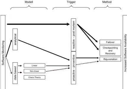
Widely accepted schemes to increase the availability of software systems either make use of redundancy in space (including failover techniques) or redundancy in time (check-pointing and restarting techniques). Most frequently these schemes are triggered following a reactive post mortem pattern. This means after an error has occurred, the method is triggered and tries to reset the system state to a known error free state and/or limit the damage to other parts of the system. However, the cost associated with a reactive scheme can be high. Redundancy in time exhausts resources like I/O and CPU capacity while redundancy in space is expensive due to extra hard- and software. Clearly there are limits to increasing system availability using reactive schemes. Promising approaches to overcome these limitations are proactive methods. One approach that has received considerable attention is rejuvenation of system parts [Huang et al. 1995]. This scheme anticipates the formation of erroneous states before it actually materialises into a failure. The listed schemes to increase system availability can be a more effective weapon if applied intelligently and preventively. The question remains when should we apply checkpointing and rejuvenation techniques.

To answer this question we need a way to tell if the current state of the system is going to evolve into a failure state. We can extend this concept to include parts or the entire history of the systems

Figure 1: Increased software availability by employing a model driven proactive preventive scheme. Solid lines represent currently employed techniques dotted lines signal the approach favoured in this paper. The boldness of lines signals the prevalence of the methods in current research.

IncreasedSoftware Availability

Rejuvenation Failover

reactive–post mortemproactive-prvventive

analytical

Linear

Software Monitoring

Chaos Theory

Modell Trigger Method

Checkpointing and Recovery

databased

Non-linear

state transitions. So to answer the question of the ideal trigger timing for high availability schemes we need to develop a model of the system in question which allows us to derive optimised triggering times.

To increase availability of a software system during runtime basically three steps are involved:

The method to (re)-initiate a failure free state-space, the trigger mechanism to select and start a method and the type of model which is employed by the trigger mechanism. In the following paragraphs we will briefly review these steps.

2.1 Modelling Schemes

General schemes to improve software availability include check-pointing, recovery and failover techniques which have been review extensively in literature. More recently software rejuvenation has been established. This procedure counteracts the ageing process of software by restarting specific components. Software ageing describes misbehaviour of software that does not cause the component to fail immediately. Memory leaks but also bugs that cannot be completely recovered from are two examples. Rejuvenation is based on the observation, that restarting a component during normal operation is more efficient than frequently check-pointing the systems state and restarting it after the component has failed.

Clearly, we favour proactive preventive schemes over reactive schemes, because of their promise to increase system availability without waiting for an error to happen. But how do we know when a failure is to occur so that we can employ any of the general techniques to avoid the lurking error? One approach is to build a model of the software system in question. Ideally, this model tells us in which state the real system should be so we can compare and base our decision on employing an error avoidance strategy based on the model. In a less ideal world the model should give us at least a probabilistic measure to estimate the probability of an error occurring within a certain time frame.

Indeed this is the approach described in this paper.

2.2 Analytical Modelling

Analytical continuous time Markov chain model for a long running server-client type telecommunication system where investigated by Huang et al. [Huang et al. 1995]. They express downtime and the cost induced by downtime in terms of the models parameters. Dohi et al. relax the assumptions made in Huang of exponentially distributed time independent transition rates (sojourn time) and build a semi-Markov model [Dohi et al. 2000]. This way they find a closed form expression for the optimal rejuvenation time. Garg et al. develop Markov regenerative stochastic Petri Nets by allowing the rejuvenation trigger to start in a robust state [Garg et al. 1995 ]. This way they can calculate the rejuvenation trigger numerically.

One of the major challenges with analytical approaches is that they do not track changes in system dynamics. Rather the patterns of changes in the system dynamics are left open to be interpreted by the operator. An improvement on this type of fault detection is to take changes into account and use these residuals to infer faulty components [Frank 1990], [Patton et al. 1989]. However, analytical approaches are not practical when confronted with the degree of complexity of software systems in use.

2.3 Data-based Modelling

Literature on measurement-based approaches to modelling software systems has been dominated by approaches limited to a single or few observable variables not considering feature detection methods.

Most models are either based on observations about workload, time, memory or file tables. Garg et al.

propose a time-based model for detection of software ageing [Garg et al. 1998]. Vaidyanathan and Trivedi propose a workload-based model for prediction of resource exhaustion in operating systems and conclude that measurement-based software rejuvenation outperforms simple time statistics [Vaidyanathan et al. 1999]. Li et al. collect data from a web server which they expose to an artificial workload [Li et al. 2002]. They build time series ARMA (autoregressive moving average) models to detect ageing and estimate resource exhaustion times. Chen et al. propose their Pinpoint system to monitor network traffic [Chen et al. 2002]. They include a cluster-based analysis technique to correlate failures with components and determine which component is most likely to be in a faulty

state. Salfner et. al build on log files as a valuable resource for system state description [Salfner et al.

2004]. We apply pattern recognition techniques on software events to model the system’s behaviour in order to calculate probability distribution of the estimated time to failure.

3 Learning Task

The learning task in our scenario is straightforward. Given a set of labelled observations we compute a classifier by a learning algorithm that predicts the target class label which is either “failure” or “no failure”. As the classifier mechanism, we employ universal basis functions (UBF) and discrete time Markov chain (DTMC) with time as additional state information.

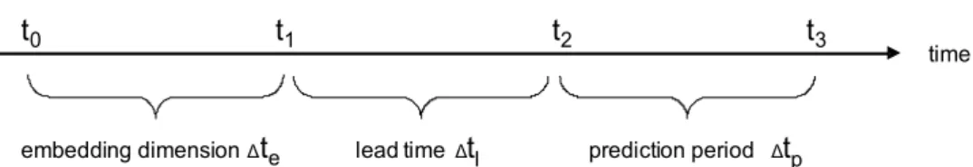
We say a prediction at time t₁ is correct if the target event occurs at least once within the prediction

period tp. The prediction period occurs some time after the prediction is made, we call this the lead time tl. This lead time is necessary for a prediction to be of any use. The prediction period defines

how far the prediction extents into the future. The value of the lead time tl critically depends on the problem domain, e.g., how long does it take to restart a component or to initiate a fail over sequence.

The value of the prediction period can be adapted more flexibly. The larger this value becomes the easier the prediction problem, but the less meaningful the prediction will be. The embedding dimension te specifies how far the observations extend into the past.

Figure 2: The embedding dimension specifies how far the labelled observations extend into the past. The lead time specifies how long in advance a failure is signalled. A prediction is correct if the target event occurs at least once within the prediction period.

t₂ t₃

prediction period Δt_p t₁ time

lead timeΔt_l

embedding dimensionΔt_e t₀

4 Modelling Objectives

Large software systems can become highly complex and are mostly heterogeneous, thus we assume that not all types of failures can be successfully predicted with one single modelling methodology.

Therefore, we approached the problem of failure prediction from two directions. One model is operating on continuously evolving system variables (e.g., system workload or memory usage). It utilizes Universal Basis Functions (UBF) to approximate the function of failure occurrence. The DTMC model operates on event triggered data (like logged error events) and predicts failure occurrence events.

Both models use time-delayed embedding. We chose te to be ten minutes. Despite of their principle focus on continuous / discrete data both models can additionally handle data of the other domain. Another important aspect is that neither approach relies on intrusive system measurements which becomes especially important for systems built from commercial-of-the-shelf (COTS) software components.

4.1 Universal Basis Functions Approach (UBF)

To model continuous variables we employ a novel data-based modelling approach we call Universal Basis Functions (UBF) which was introduced in [Hoffmann 2004]. UBF models are a member of the class of non-linear non-parametric data-based modelling techniques. UBF operate with linear mixtures of bounded and unbounded activation functions such as Gaussian, sigmoid and multi quadratics. Non- linear regression techniques strongly depend on architecture, learning algorithms, initialisation heuristics and regularization techniques. To address some of these challenges UBF have been developed. These kernel functions can be adapted to evolve domain specific transfer functions. This makes them robust to noisy data and data with mixtures of bounded and unbounded decision regions.

UBF produce parsimonious models which tend to generalise more efficiently than comparable approaches such as Radial Basis Functions [Hoffmann 2004b].

4.2 Discrete Time Markov Chain Approach

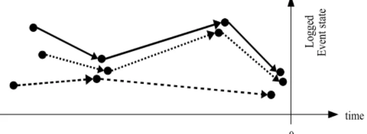
Our approach for modelling discrete, event triggered data starts from a training data set consisting of logged events together with additional knowledge when failures have occurred. Events preceding each failure are extracted and aligned at the failure's occurrence times (t=0). For illustrative purposes we map the multidimensional event feature vector onto a plane in Figure 3.

Starting at t=0 we apply a clustering algorithm to join events with similar states. Each group forms a state cluster defined by the event states and the time to failure of the constituting events. Figure 4 depicts the clustering result.

For clustering we use the sections of data preceding failures. This yields conditional probabilities of failure occurrences. In order to drop this limitation the overall training data set is used to estimate relative frequencies for each state cluster transition.

Online failure prediction is about calculating the probability of and the time to any failure's occurrence. Therefore, the calculation's result is a function P_Ft. The first step to determine P_Ft is to identify the set of potential state clusters the system might be in, depending on past events (time delayed embedding). From the backward clustering algorithm we can assure the Markov property that future states depend only on the current state. Therefore, the probability P_Ft can be

Figure 3: Preceding events of three failures. For illustrative purposes we map the multidimensional event feature vector onto a plane.

0

time Logged Event state

Figure 4: Similar events form state ranges

0

time

Event state

calculated with a discrete time Markov chain (DTMC). We take only state clusters into account which contribute to a failure at time t.

4.3 Variable Selection / Feature Detection

Generalisation performance of a model is closely related to the number of free parameters in the model. Selecting too few as well as selecting too many free parameters can lead to poor generalisation performance [Baum et al. 1989], [Geman et al. 1992]. For a complex real-world learning problem, the number of variables being monitored can be prohibitively high. There is typically no a-priori way of determining exactly the importance of each variable. The set of all observed variables may include noisy, irrelevant or redundant observations distorting the information set gathered. In the context of optimal rejuvenation schedules for example, the variables load and slope of resource utilisation are frequently employed as explanatory variables [Trivedi et al. 2000], [Dohi et al. 2000]. But how do we know which variables contribute most to the model quality?

In general we can distinguish between two approaches: the filter and the wrapper approach. In the filter approach the feature selector serves to filter out irrelevant attributes [Almuallim et al. 1994].

It is independent of a specific learning algorithm. In the wrapper approach the feature selector relies on the learning algorithm to select the most important features. Although the wrapper approach is not as general as the filter approach, it takes into account specifics of the underlying learning mechanism.

This can be disadvantageous because of possible biasing towards certain variables. The major advantage of the wrapper approach is that it utilizes the induction algorithm itself as a criterion and the purpose is to improve the performance of the underlying induction algorithm. In each category feature selection can be further classified into exhaustive and heuristic searches. Exhaustive search is, except for a very few examples, infeasible. So we are basically limited to heuristic approaches trying to include as much information about the variable set as possible.

In this paper we employ the probabilistic wrapper approach as developed in [Hoffmann 2004].

Basically this procedure starts with a random search in the variable space and keeps the variable combinations which yield better than average model quality. These variable combinations are fed back

into the pool of available variables thus increasing the probability that they will be drawn again. This procedure has been shown to be highly effective.

4.4 Rare Event Prediction

Large volumes of data containing small numbers of target events have brought importance to the problem of effectively mining rare events. In domains such as early fault detection, network intrusion detection and fraud detection a large number of events occur, but only very few of these events are of actual interest. This problem is sometimes also called the skewed distribution problem. Given a skewed distribution of observations, we would like to generate a set of labelled observations with a desired distribution. The desired distribution is the one we assume would maximize our classifier performance, without removing any observations. We found that determining the right distribution is somewhat of an experimental art and requires extensive empirical testing. One frequently applied approach is replicating the minority class to achieve a desired distribution of learning pattern [Chan et al. 1999]. This approach is intuitively comprehensible; it fills up the missing observations by replicating known ones until we get a desired distribution of events. Another approach are boosting algorithms which iteratively learn differently weighted, respectively skewed samples [Joshi et al.

2001A], [Freund et al. 1997]. In our approach we focus on evenly distributed sets of observations and re-sample the minority class to get evenly distributed classes.

5 Metrics

In measuring the performance of our models we must distinguish between the performance of the statistical model and the performance of the classifier. In many instances we create models that do not

directly tell us if and when a failure is to occur in the observed system, even though this may be our primary goal. The model may predict, for instance, that the likelihood of an error occurring within a certain future time frame may be 10%, but it is up to our interpretation if we take any action on that result or not. Thus we adopt two different sets of performance measures: one to assess the statistical model quality and the second set to assess the performance with respect to the number of correctly predicted failures (true positives), missed failures (false negatives) and also to the number of

incorrectly predicted failures (false positives). To assess statistical properties of our models we employ a root-mean-square error [Weigend et al. 1994], [Hertz et al. 1991], [Bishop 1995].

In our sample data we count 96 failure occurrences within 1080 observations. The majority class thus contains 984 observations not indicating any failure; the minority class contains 96 entries. By always considering the majority class we would achieve a predictive accuracy of roughly 89%. Thus the predictive power of the widely used quality metric predictive accuracy is of limited use in a scenario where we would like to model and forecast rare events – they yield an overly optimistic model quality. Therefore, we need a metric optimised for rare event classification rather than predictive accuracy. We employ precision, recall, the integrating F-Measure and cumulative cost as described in the next sections.

5.1 Precision, Recall and F-Measure

Precision and recall, originally defined to evaluate information retrieval strategies, are frequently used to express the classification quality of a given model. They have even been used for failure modelling.

Applications can be found for example in Weiss [Weiss 1999] and [Trivedi et al. 2000]. Precision is the ratio between the number of correctly identified failures and predicted failures:

positives false

positives true

positives true

  precision

Recall is defined as the ratio between correctly identified faults and actual faults. Recall sometimes is also called sensitivity or positive accuracy.

negatives false

positives true

positives true

  recall

Following Weiss [Weiss 1999] we use reduced precision. There is often tension between a high recall and a high precision rate. Improving the recall rate, i.e. reducing the number of false negative alarms, mostly also decreases the number of true positives, i.e. reducing precision. A widely used metric which integrates the trade-off between precision and recall is the F-Measure [Rijsbergen 1979].

recall precision

recall precision





2 Measure -

F

5.2 Cost-based Measures

In many circumstances not all prediction errors have the same consequences. It can be advantageous not to strive for the classifier with fewest errors but the one with the lowest cost. Cost-based metrics have been explored by [Joshi et al. 2001A], [Stolfo et al. 2000] and [Chan et al. 1999] for intrusion detection and fraud detection systems. Trivedi et al. explore a cost-based metric to calculate the monetary savings associated with a certain model by assigning monetary savings to a prevented failure and cost to failures and false positive predictions [Trivedi et al. 2000]. This type of metric takes into account that failing to predict a rare event can impose considerably higher cost than making a false positive prediction. I.e., cost can be associated with monetary or time units. Assume that a failure within a telecommunication platform causes the system to malfunction and to violate guaranteed characteristics such as response times. If the failure can be forecast and with a probability P be avoided, that prediction would decrease potential liabilities. If the failure had not been forecast and the system had gone down then it would have generated higher costs. Vice versa each prediction (both false and correct) also generates additional costs. For example, due to many unnecessary restarts the platform may be busy and would reject calls.

6 Modelling a Real-world System

Both modelling techniques presented in this paper have been applied to data of a commercial telecommunication platform. The primary objective was to predict failures in advance.

The main characteristics of the software platform investigated in this paper are its component- based software architecture running on top of a fully featured clustering environment consisting of two to eight nodes. We measured test data of a two node cluster non-intrusively using existing logfiles:

Error logs served as source for event triggered data and logs of the operating system level monitoring tool SAR for time continuous data. To label the data sets we had access to the external stress generator keeping track of both the call load put onto the platform and the time when failures occurred during

system tests. We have monitored 53 days of operation over a four month period providing us with approximately 30GB of data. Results presented in the next section originate from a three days excerpt.

We split the three days of data into equally proportioned segments (one day per segment). One data segment we use to build the models, the second segment we use to cross validate the models, the third segment is our test data which we kept aside. Our objective is to model and predict the occurrence of failures up to five minutes ahead (lead time) of their occurrence.

We gathered the numeric values of 42 operating system variables once per minute and per node.

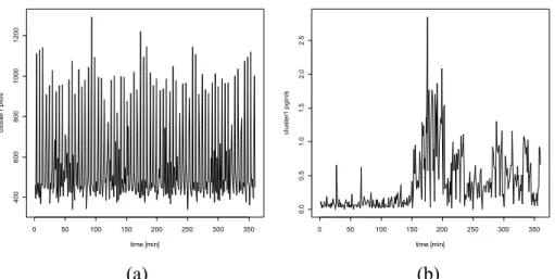
This leaves us with 84 variables in a time series describing the evolution of the internal states of the operating system, thus in a 24-hour period we collect n = 120.960 readings. Figure 6 Depicts plots of two variables over a time period of six hours. Logfiles were concurrently collected with continuous measurements and the same three days were selected for modelling and testing. System logfiles contain events of all architectural layers above the cluster management layer. The large variety of logged information includes 55 different, partially non-numeric variables in the log files as can be seen

0 50 100 150 200 250 300 350

40060080010001200

time [min]

cluster1 pflt/s

0 50 100 150 200 250 300 350

0.00.51.01.52.02.5

time [min]

cluster1 pgin/s

Figure 6: Showing two SAR system variables over a sample period of six hours. (a) shows page faults per second on node one, (b) shows pages-in per second

(a) (b)

Figure 5: One error log record consisting of three log lines

2004/04/09-19:26:13.634089-29846-00010-LIB_ABC_USER-AGOMP#020200034000060|

0201010444300000|0000000000000000-020234f43301e000-2.0.1|0202000003200060|00000001 2004/04/09-19:26:13.634089-29846-00010-LIB_ABC_USER-NOT: src=ERROR_APPLICATION

sev=SEVERITY_MINOR id=020d02222083730a

2004/04/09-19:26:13.634089-29846-00010-LIB_ABC_USER-unknown nature of address value specified

in Figure 5. The amount of log data per time unit varies greatly: The frequency ranges from two to 30.000 log records per hour. A noteworthy result is that there is no one-to-one mapping between log- record frequency and the failure probability suggesting that trivial models would not work in this environment.

7 Results

Results presented in this paper are based on a three day observation period. We investigate the quality of our models regarding failure prediction performance. In order to rank our results we compare them with two straightforward modelling techniques applied to the same data: Naive forecasting after a fixed time interval and forecasting using a linear ARMA model.

7.1 Precision, Recall and F-Measure

We calculated precision, recall and F-measure for predictions with the test data. The linear ARMA was fed with SAR data. The model did not correctly predict any failure in the observation period, precision and recall values could thus not be calculated. The naive model was calculated by using the mean delay between failures in the training data set which was 65 minutes. We used this empirical delay to predict failures on unseen test data.

7.2 Cumulative Cost of Operations

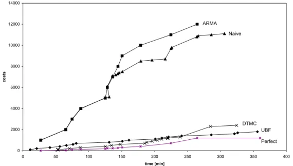
To evaluate the cost associated with each model we assign a value to failure prevention (true positive = 100), false prediction (false positive = 100) and missed failures (false negative = 1.000).

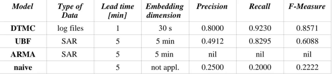
Model Type of Data

Lead time [min]

Embedding dimension

Precision Recall F-Measure

DTMC log files 1 30 s 0.8000 0.9230 0.8571

UBF SAR 5 5 min 0.4912 0.8295 0.6088

ARMA SAR 5 5 min nil nil nil

naive 5 not appl. 0.2500 0.2000 0.2222

Table 1: Precision, recall and F-Measure for discrete time Markov chain (DTMC), universal basis function approach (UBF), auto regressive moving average (ARMA) and naive model. In the case of UBF we report mean values. The linear ARMA model did not correctly predict any failure in the observation period, precision and recall values could thus not be calculated. The reported results where generated on previously unseen test data.

These values are admittedly somewhat arbitrary and can be adjusted to reflect the individual characteristics of the system in question. In a production system one may assign monetary values to indicate the economic benefit of failure prediction and prevention. By integrating over time and failures we arrive at a function indicating the accumulated cost introduced by the respective modelling procedure as depicted in Figure 7. Clearly, UBF and DTMC outperform the naive and the linear ARMA approach. In the case of perfect foresight we would arrive at the cost function labelled

“perfect”. All values reported are calculated with previously unseen test data.

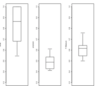
7.3 Statistical Assessment of the UBF model

To assess statistical stability of our UBF models we calculate the median and quantiles of the expected model error. We employ a stochastic optimisation procedure as discussed in [Hoffmann 2004]. We report statistical assessment of precision, recall and F-Measure as Box-Whisker plots in . All values were calculated on previously unseen test data.

Figure 7: Cost scenario for our system if we apply hypothetical costs to correctly, incorrectly and not at all predicted failures. “Perfect” is our hypothetical cost model if we had perfect foresight. The UBF and DTMC models clearly outperform the naive and linear ARMA approach .

0 2000 4000 6000 8000 10000 12000 14000

0 50 100 150 200 250 300 350 400

time [min]

costs

Naive ARMA

DTMC UBF Perfect

8 Availability Improvement

In theory forecasting failures can help to improve availability by increasing mean-time-to-failure (MTTF). Based on the results presented in Section 6 we calculate the effects of our prediction results on MTTF and availability respectively. As reported in Table 1 we get values for precision and recall of 49% and 82% for a five minute lead-time. Assuming that an arbitrary system exhibits one tenth of an hour (six minutes) downtime per 1000 hours of operation (which corresponds to a “four nines”

availability) the application of our failure prediction technique would increase MTTF from 999.9 hours to 5555 hours of operation. Given the increased MTTF we get:

A= MTTF

MTTFMTTR= 5555

55550.1≈0.999982

which is close to an order of magnitude better than without failure prediction. Where MTTR is mean time to repair and A is availability. In complex real systems, failure prevention will of course not be able to avoid all failures even if they had been predicted correctly. Even worse, false alarms may evoke additional failures. It will be a challenge for future investigations to find out more about these effects.

Figure 8: Box-Whisker plots of recall, precision and F-Measure for the UBF model applied to previously unseen test data. Shown are the mean, minimum, maximum and quantiles of the respective measure The F-Measure is a cumulative measure integrating precision and recall into a single value.

0.30.40.50.60.70.80.91.0

recall 0.30.40.50.60.70.80.91.0

precision 0.30.40.50.60.70.80.91.0

F-Measure

9 Conclusion and Future Work

The objective of this paper was to model and predict failures of complex software systems. To achieve this we introduced two novel modelling techniques. These are a discrete time Markov chain (DTMC) models with time as additional state information and Universal Basis Functions (UBF). DTMC are easier to interpret than UBF while the latter are more robust to noisy data and generalize more efficiently.

We measured data from a commercial telecommunication platform. In total we captured 84 time continuous variables and 55 error log file variables. For modelling purposes an excerpt of three days has been taken. To reduce the number of variables we employed a probabilistic feature detection algorithm. Event driven error log files were modelled with DTMC and time continues operating system observations with the UBF approach. We reported the models' quality as recall, precision, F- Measure and cumulative cost. Our results were compared with a naive and a linear ARMA modelling approach.

Our results indicate superior performance of the DTMC and UBF models. In particular we outperform the naive approach by a factor of three to four in terms of the F-Measure and by a factor of five with respect to cumulative cost. Assuming that all forecast failures can be avoided our modelling techniques may lead to an order of magnitude improvement of system availability. The DTMC model achieves best performance for smaller lead times. Larger lead times are best captured by the UBF model.

Future work will include research on the validity of our models depending on system configuration. Additional benefits may also arise from interpreting our models for root cause analysis.

Both modelling techniques have the potential to integrate continuous and event driven data and may additionally be combined into a single model. Future research will have to show if this leads to improved model quality.

References

[Almuallim et al. 1994] : Almuallim, H., Dietterich, T. G. . Learning boolean concepts in the presence of many irrelevant features. Artificial Intelligence, 69():, 1994

[Baum et al. 1989] : Baum E., Haussler D.. What size net gives valid generalisation?. Neural computation, 1(1):

151-160, 1989

[Bishop 1995]: Bishop C. M.. Neural Networks for Pattern Recognition. Clarendon Press, London, 1995 [Candea et al. 2003] : G. Candea and M. Delgado and M. Chen and A. Fox, Automatic Failure-Path Inference: A

Generic Introspection Technique for Internet Applications, Proceedings of the 3rd IEEE Workshop on Internet Applications (WIAPP), 2003

[Chan et al. 1999] : Chan P.K., Fan W., Prodromidis A., Stolfo S.. Distributed Data Mining in Credit Card Fraud Detection. IEEE Intelligent Systems, 11(12):, 1999

[Chen et al. 2002] : Chen Mike , Emre Kiciman, Eugene Fratkin, Armando Fox and Eric Brewer (2002), Pinpoint: Problem Determination in Large, Dynamic Systems, Proceedings of 2002 International Performance and Dependability Symposium, Washington, DC, , 2002

[Dohi et al. 2000] : Dohi Tadashi , Go¡seva-Popstojanova Katerina, Trivedi Kishor S.. Statistical Non- Parametric Algorithms to Estimate the Optimal Software Rejuvenation Schedule. , ():, 2000

[Dohi et al. 2000] : Dohi Tadashi , Go¡seva-Popstojanova Katerina, Trivedi Kishor S., Statistical Non- Parametric Algorithms to Estimate the Optimal Software Rejuvenation Schedule, Dept. of Industrial and Systems Engineering, Hiroshima University, Japan and Dept. of Electrical and Computer Engineering, Duke University, USA, 2000

[Frank 1990] : Frank, P.M.. Fault Diagnosis in Dynamic Systems Using Analytical and Knowledge-based Redundancy - A Survey and Some New Results. Automatica, 26(3):459-474, 1990

[Freund et al. 1997] : Freund Y., Schapire R.. A decision theoretic generalisation of on-line learning and an application to boosting . Journal of computer and system science, 55(1):119-139, 1997

[Garg et al. 1995 ] : Garg S., A. Puliafito M. Telek and K. S. Trivedi, Analysis of Software Rejuvenation using Markov Regenerative Stochastic Petri Net, Proc. of the Sixth IEEE Intl. Symp. on Software Reliability Engineering, Toulouse, France, 1995

[Garg et al. 1998] : Garg S., Puliofito A., Telek M., Trivedi K., Analysis of preventive Maintenance in Transaction based Software Systems, , 1998

[Geman et al. 1992] : Geman S., Bienenstock E., Doursat R.. Neural Networks and the Bias/Variance Dilemma.

Neural computation, 4(1):1-58, 1992

[Gray et al. 1991] : Gray J., Siewiorek D.P. . High Availability computer systems. IEEE Computers, 9():39-48, 1991

[Gray J. 1986] : Gray J. , Why do computers stop and what can be done about it?, 5th Symposium on reliability in distributed software and database systems, LA, 1986

[Gray J. 1990] : Gray J. . A census of Tandem system availability between 1985 and 1990. IEEE Transactions on reliability, 39():, 1990

[Grey 1987] : Grey B.O.A. . Making SDI software reliable through fault tolerant techniques. Defense Electronics, 8():77-80, 85-86, 1987

[Hertz et al. 1991]: Hertz J., Krogh P., Palmer R.. Introduction to the Theory of Neural Computation. Addison Wesley, , 1991

[Hoffmann 2004] : Günther A. Hoffmann, Adaptive Transfer Functions in Radial Basis Function Networks (RBF), to appear in: International Conference on computational science, 2004

[Hoffmann 2004b] : Günther A. Hoffmann, Data specific mixture kernels in Basis Function networks, submitted for publication, 2004

[Huang et al. 1995] : Huang Y., C. Kintala, N. Kolettis and N. Fulton, Software Rejuvenation: Analysis, Module and Applications, In Proc. of the 25th IEEE Intl. Symp. on Fault Tolerant Computing (FTCS-25), Pasadena, CA, 1995

[Joshi et al. 2001A]: Joshi M., Kumar V., Agarwal R., Evaluating Boosting Algorithms to Classify Rare Classes: Comparison and Improvements,IBM 2001,

[Li et al. 2002] : Li L., Vaisyanathan, Trivedi , An Approach for Estimation of Software Aging in a Web Server, , 2002

[Patton et al. 1989]: Patton, R.J., P.M. Frank and R.N. Clark. Fault Diagnosis in Dynamic Systems: Theory and Applications. Prentice-Hall, , 1989

[Rijsbergen 1979]: Rijsbergen Van C.J.. Information Retrieval. Butterworth, London, 1979

[Salfner et al. 2004] : Salfner F, Tschirpke S and Malek M, Logfiles for Autonomic Systems, Proceedings of the IPDPS 2004, 2004

[Scott 1999]: Scott D. , Making smart investments to reduce unplanned downtime. , Tactical Guidelines Research Note Note TG-07-4033, Gartner Group, Stamford, CT, 1999

[Stolfo et al. 2000] : Stolfo S., Fan W., Lee W., Cost-based Modeling for Fraud and Intrusion Detection: Results from the JAM Project , DARPA Information Survivability Conference & Exposition, 2000

[Sullivan et al. 2002]: Sullivan,Chillarege, Software Defects and their Impact on System Availability - A Study of Field Failures in Operating Systems, 2002,

[Trivedi et al. 2000] : Trivedi Kishor S., Vaidyanathan Kalyanaraman and Go¡seva-Popstojanova Katerina, Modeling and Analysis of Software Aging and Rejuvenation, , 2000

[Vaidyanathan et al. 1999] : Vaidyanathan K. and K. S. Trivedi, A Measurement-Based Model for Estimation of Resource Exhaustion in Operational Software Systems, Proc. of the Tenth IEEE Intl. Symp. on Software Reliability Engineering, Boca Raton, Florida, 1999

[Weigend et al. 1994]: Weigend A. S., Gershenfeld N. A., eds. . Time Series Prediction. Addison Wesley, , 1994

[Weiss 1999] : Weiss G. M., Timeweaver: a Genetic Algorithm for Identifying Predictive Patterns in Sequences of Events, , 1999