Contents lists available atScienceDirect
Polar Science
journal homepage:www.elsevier.com/locate/polar
Comparative simulations of the evolution of the Greenland ice sheet under simplified Paris Agreement scenarios with the models SICOPOLIS and ISSM
Martin Rückamp
a,∗, Ralf Greve
b, Angelika Humbert
a,caAlfred Wegener Institute Helmholtz Centre for Polar and Marine Research, Bremerhaven, Germany
bInstitute of Low Temperature Science, Hokkaido University, Sapporo, Japan
cDepartment of Geosciences, University of Bremen, Bremen, Germany
A R T I C L E I N F O Keywords:
Greenland ice sheet Paris Agreement Sea level rise Ice sheet modelling Uncertainty assessment
A B S T R A C T
Projections of the contribution of the Greenland ice sheet to sea level rise comprise uncertainties that arise from the imposed climate forcing and from the underlying mathematical and numerical description used by ice flow models. Here, we present a comparative modelling study with the models SICOPOLIS, using the shallow ice approximation (SIA) on a structured grid, and ISSM, using a higher-order (HO) approximation of the Stokes equation on an unstructured grid. Starting from a paleoclimatic spin-up produced by SICOPOLIS, the models are forced with two different, simplified warming scenarios based on RCP2.6 projections from climate models, which are in line with the limit of global warming negotiated for the Paris Agreement. ISSM/HO produces lower flow speeds at the glacier termini, but more acceleration in narrow outlet glaciers compared to SICOPOLIS/SIA.
This leads to a larger elevation reduction for ISSM/HO, and thus a positive feedback on the surface mass balance (with that of ISSM/HO becoming ∼50 Gt a−1more negative). Across the two models and scenarios, the pro- jected mass loss by 2300 is ∼62–88 mm sea level equivalent.
1. Introduction
A major consequence of climate change is global sea level rise, which has just recently been shown to accelerate (Nerem et al., 2018).
The Greenland ice sheet has contributed about 20% to sea level rise during the last decade (Rietbroek et al., 2016) and, holding in total an ice mass of ∼7.36 m sea level equivalent (SLE) (Bamber et al., 2013), its future contribution poses a major societal challenge. The mass loss of the ice sheet has two main contributions: changes in the surface mass balance (SMB) and increasing discharge due to acceleration of outlet glaciers. For the past decades, the relative contributions are estimated to about 60% and 40%, respectively (van den Broeke et al., 2016).
Understanding the processes determining the future mass loss of the ice sheet is essential for predicting its contribution to future sea level rise.
Previous efforts like SeaRISE (Bindschadler et al., 2013;Nowicki et al., 2013), ice2sea (Gillet-Chaulet et al., 2012) and, most recently, initMIP-Greenland (Goelzer et al., 2018) have revealed the sensitivity of current ice sheet models to external forcing under standardized sce- narios, which gives rise to large uncertainties. The differences in model response are attributed to different ice dynamics approximations, nu- merics, spatial resolution, and initialization methods. As a consequence, projections for ice sheet evolution in the next 100–300 years still show
a wide spread, and hence limit subsequent impact analysis concerning, e.g., regional sea level change and coastal erosion.
Comparisons targeting specifically the impact of different ice dy- namics approximations on predictions of ice sheet contribution to sea level rise are scarce and partly contradictory.Seddik et al. (2012)ap- plied the ice flow models Elmer/Ice with full Stokes (FS) dynamics and SICOPOLIS with the shallow ice approximation (SIA) to the entire Greenland ice sheet, forced by scenarios from SeaRISE. They found that the ice sheet mass loss is more sensitive with FS than with SIA for the dynamical forcing (doubled basal sliding) experiment, but less sensitive for the direct global warming scenario. Similarly,Seddik et al. (2017) conducted a comparative regional modelling study of the Shirase drainage basin, East Antarctica, with a single model (Elmer/Ice) oper- ated in either FS or SIA mode. Forced by SeaRISE scenarios, they re- ported a negligible difference in model response for the surface climate experiment, while, for the increased basal sliding experiment, the ice volume change is ∼30% larger for SIA than for FS.Fürst et al. (2013) studied the centennial evolution of the entire Greenland ice sheet by using five approximations to the force balance, ranging between SIA and the Blatter–Pattyn higher-order (HO) approximation (Blatter, 1995;
Pattyn, 2003). Their results show that the inclusion of membrane stress gradients actually reduces the volume loss by up to 20% compared to
https://doi.org/10.1016/j.polar.2018.12.003
Received 2 July 2018; Received in revised form 12 November 2018; Accepted 4 December 2018
∗Corresponding author.
E-mail addresses:martin.rueckamp@awi.de(M. Rückamp),greve@lowtem.hokudai.ac.jp(R. Greve),angelika.humbert@awi.de(A. Humbert).
Polar Science 21 (2019) 14–25
Available online 07 December 2018
1873-9652/ © 2018 The Authors. Published by Elsevier B.V. This is an open access article under the CC BY-NC-ND license (http://creativecommons.org/licenses/BY-NC-ND/4.0/).
T
the SIA approach.
Here, we analyse the uncertainty arising from model physics, nu- merical techniques and implementation in projections of the Greenland mass loss up to the year 2300. For this purpose, we choose two different ice dynamics approximations and two different discretization schemes, realized in the models SICOPOLIS (Greve and Herzfeld, 2013; Greve and Blatter, 2016) and ISSM (Larour et al., 2012). The scenarios are based on the 2015 United Nations Climate Change Conference (COP21), where it was negotiated to limit global warming to well below 2.0°C and, if possible, to 1.5°C above pre-industrial levels by the end of this century (Paris Agreement). This is often interpreted as allowing for a potential warming overshoot within this century, before settling at a maximum of 1.5°C (Rogelj et al., 2015). The interim overshoot may strongly affect the mass balance of the Greenland ice sheet. Whether or not the political target will be met, it is expected that the ice sheet will lose substantial mass (IPCC, 2018), and we aim at assessing the un- certainty in mass loss projections arising from our two different models.
To achieve this goal, we construct simplified Representative Con- centration Pathway (RCP) 2.6 forcing scenarios with and without in- terim overshoot based on climate data output from general circulation models (GCMs), and investigate the response of the two ice sheet models to these scenarios.
2. Ice sheet models
2.1. SICOPOLIS
SICOPOLIS (SImulation COde for POLythermal Ice Sheets; www.
sicopolis.net) is a dynamic/thermodynamic ice sheet model that was originally created byGreve (1997)for the Greenland ice sheet. Since then, the model has been developed continuously, and the latest ver- sion, used in this study, is 5-dev (“developmental”). It is based on finite- difference solutions of the SIA for grounded ice (Hutter, 1983;Morland, 1984), the shallow shelf approximation (SSA) for floating ice (Morland, 1987;MacAyeal, 1989) and, optionally, hybrid SIA/SSA dynamics for ice streams (Bernales et al., 2017). For this study, we use only the SIA mode for grounded ice. The description given here followsGreve and Herzfeld (2013)closely.
A particular feature of SICOPOLIS is its very detailed treatment of ice thermodynamics. A variety of different thermodynamics solvers are available, namely the polythermal two-layer method, two versions of the one-layer enthalpy method, the cold-ice method and the isothermal method. For the experiments of this study, we use the one-layer melting-CTS enthalpy scheme (Greve and Blatter, 2016).
SICOPOLIS allows different options for the ice rheology. Here, we use the regularized Glen flow law in the formulation by Greve and Blatter (2009). The temperature-dependent rate factor for cold ice is by Cuffey and Paterson (2010, Sect. 3.4.6), and the water-content-depen- dent rate factor for temperate ice is byLliboutry and Duval (1985). The ice surface is assumed to be traction-free. Basal sliding under grounded ice, vb, is described by a Weertman-type sliding law with sub-melt sliding, similar toGreve and Herzfeld (2013):
= v T C e
( ) T Npq,
b b b b
b b
(1) wherepandqare the sliding exponents,Cbis the sliding coefficient, γ the sub-melt-sliding parameter, b the basal drag (shear stress), the basal normal stress (ice stress minus water pressure, counted positive for compression) andTb the basal temperature relative to pressure melting (in °C, always ≤ 0°C). In order to avoid unrealistically high sliding velocities for almost floating ice, we do not allow to fall below a
minimum of 0.35×the normal stress exerted by the ice load [Sato and Greve (2012)used a limiting factor of 0.2 in a modelling study for the Antarctic ice sheet; this was found to be insufficient here to keep the velocities within a reasonable limit]. The physical parameters are listed inTable 1.
The model domain for the Greenland ice sheet covers the entire area of Greenland and the surrounding oceans. We use the EPSG:3413 grid, based on a polar stereographic projection with the WGS 84 reference ellipsoid, standard parallel70 Nand central meridian45 W. The ste- reographic plane is spanned by the Cartesian coordinatesxandy, and the coordinatezpoints upward. The bed topography is BedMachine v3 (Morlighem et al., 2017). Glacial isostatic adjustment (GIA) for the paleoclimatic spin-up (see below, Sect. 3.1) is modelled by the local- lithosphere–relaxing-asthenosphere (LLRA) approach with a time lag
=3000 a
iso (Le Meur and Huybrechts, 1996), while the lithosphere is kept fixed (no GIA) for the future climate experiments of this study. The geothermal heat flux is byGreve (2019), an update of the distribution by Greve and Herzfeld (2013) based on a global representation by spherical harmonics, combined with information from five Greenlandic deep ice cores and three rock-borehole measurements. It is applied 2 km below the ice base in order to account for the thermal inertia of the lithosphere (Ritz, 1987).
The stereographic plane is discretized by a regular (structured) grid with 5 or 10 km resolution. In the vertical, we use terrain-following coordinates (sigma transformation) with 81 layers in the ice domain and 41 layers in the thermal lithosphere layer below. The ice front can advance or retreat freely on the available land area, but it is not allowed to advance into the sea. Due to the SIA dynamics, a special boundary condition at the ice front is not required.
2.2. ISSM
The second model applied here is the Ice Sheet System Model (ISSM;
Larour et al., 2012). As we want to focus on differences in model re- sponse arising from the ice dynamics approximation and numerical techniques/implementation (including grid resolution), we aim at Table 1
Physical parameters used for SICOPOLIS and ISSM (largely following the SICOPOLIS settings for initMIP-Greenland;Goelzer et al., 2018).
Quantity Value
Density of ice, ρ 910 kg m 3
Gravitational acceleration,g 9.81 m s 2
Length of year,1 a 31 556 926 s
Power law exponent,n 3
Residual stress, 0 10 kPa
Flow enhancement factor,E 3
Melting temperature
at low pressure,T0 273.16 K
Clausius-Clapeyron gradient, β 8.7×10⁴K m1
Universal gas constant,R 8.314 Jmol K1 1
Heat conductivity of ice,κ 9.828 e 0.0057 [K]T W m K1 1 Specific heat of ice,c (146.3+7.253 [K]) Jkg KT 1 1
Latent heat of ice,L 3.35×10 Jkg5 1
Sliding coefficient,Cb 6.72 m a Pa1 1
Sliding exponents,( , )p q (3,2)
Sub-melt-sliding parameter, γ 1 C
Asthenosphere density, a 3300 kg m 3
Density×specific heat of the
lithosphere, r rc 2000 kJ m K3 1
Heat conductivity of the
lithosphere, r 3 W m K1 1
making the ISSM settings as similar as possible to that of SICOPOLIS (Sect. 2.1). Among the several approximations to full Stokes flow available in ISSM, we employ the Blatter–Pattyn HO approximation to account for longitudinal and transverse stress gradients. Compared to the SIA, this approximation is computationally more expensive, but more appropriate for ice streams. For the ice thermodynamics, we also choose an enthalpy scheme, with the basal boundary conditions as developed and applied by Kleiner et al. (2015) and Bondzio et al.
(2017). The ice rheology is treated as in SICOPOLIS with a regularized Glen flow law, a temperature-dependent rate factor for cold ice, and a water-content-dependent rate factor for temperate ice. Contrary to the finite difference implementation in SICOPOLIS, the ISSM model equa- tions are solved numerically with the finite element method. Velocity, enthalpy (temperature and microscopic water content) and geometry fields are computed on each vertex of the mesh using piecewise-linear finite elements.
Basal sliding follows the Weertman-type sliding law (1) rewritten as a Neumann boundary condition (i.e., b=f v( , ))b … . The corresponding parameters are chosen as listed inTable 1. Boundary conditions at the lateral margins are the water pressure for marine-terminating glaciers, and zero pressure for land-terminating glaciers. A traction-free boundary condition is imposed at the ice/air interface. The spatial pattern of the geothermal flux is the same as in SICOPOLIS (Greve, 2019).
The ISSM model domain for the Greenland ice sheet covers the same area as in SICOPOLIS on the same EPSG:3413 grid. The bed topography is also BedMachine v3 (Morlighem et al., 2017). For all simulations performed with ISSM, the ice front is fixed in time, and a minimum ice thickness (H) of 10 m is applied. This implies that calving exactly compensates the outflow through the margins, and initially glaciated points are not allowed to become ice-free. However, regions that reach the minimum thickness are assumed in the analysis to have retreated.
Contrary to SICOPOLIS, floating ice is allowed to develop, with a freely evolving grounding line according to a sub-grid parameterization scheme, which tracks the grounding line position within the element (Seroussi et al., 2014). However, to ensure consistency with the SICOPOLIS model, no basal melting is considered under developing floating ice. No GIA model is applied.
Model calculations with ISSM are performed on a horizontally un- structured grid. To limit the number of elements while maximizing the spatial resolution in regions where physics demands higher accuracy, the horizontal mesh is generated with a higher resolution oflmin=1km in fast-flowing regions and a coarser resolution oflmax=20km in the interior. The anisotropic mesh adaptation is based on the Hessian ma- trix of the horizontal velocity field produced by the paleoclimatic spin- up with SICOPOLIS (see below, Sect. 3.1). The vertical discretization comprises 15 terrain-following layers, refined towards the base where vertical shearing becomes more important. The complete mesh com- prises 665 238 active elements, resulting in 1 961 775 degrees of freedom.
3. Model experiments
A crucial prerequisite for projections is a reasonable initial state of the ice sheet regarding ice geometry, surface velocities and englacial temperature. Different methods are currently in use for initializing ice sheets, with their various advantages and drawbacks (e.g., Goelzer et al., 2018). In order to obtain a suitable present-day configuration of the Greenland ice sheet with a well-constrained temperature field, it is desirable to carry out a paleoclimatic spin-up over at least one full glacial cycle. Since this is computationally almost prohibitive with a HO model, we conduct the spin-up with the computationally cheaper shallow-ice model SICOPOLIS only, and then interpolate the relevant fields at the end of the spin-up to the ISSM grid.
The objective of this study is to assess the differences of the two model responses arising from model physics, numerical techniques and
their implementation, rather than delivering projections based on highly detailed climate forcing scenarios. Therefore, we resolve to simplifiedRCP2.6-like scenarios with and without interim overshoot, based on RCP2.6 peak-and-decline climate data output from GCMs, and impose them as anomalies on the reference climate used in the spin-up simulation. In doing so, we bypass inter-annual variability and skills of individual GCMs to reproduce the distribution of the near-surface air temperature and precipitation over Greenland. Further, to achieve the goal mentioned above, we set up the modelling approach in a way that both models use the same initial conditions, ice rheology, sliding law and surface mass balance calculation.
3.1. Paleoclimatic spin-up with SICOPOLIS
For the present-day mean annual and July mean surface tempera- ture, we employ the parameterizations byFausto et al. (2009). These parameterizations express the temperature distributions as linear functions of surface elevation, latitude and longitude. However, the parameterizations are valid for 1996–2006, whereas our reference year (timet=0) is 1990. In order to correct for this difference, we apply an offset of −1°C to both parameterizations. This value was estimated based on the data shown by Kobashi et al. (2011,Fig. 1therein).
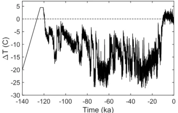
The main time-dependent driver for the paleoclimatic spin-up is the surface temperature anomaly T t( ), assumed to be spatially uniform over the Greenland ice sheet. It is based on the 18O record from the NGRIP ice core (North Greenland Ice Core Project members, 2004) on the GICC05modelext time scale (Wolff et al., 2010), converted to tem- perature with the T/ 18Otransfer factor of2.4 C ‰1byNielsen et al.
(2018) (based onHuybrechts, 2002). Warming during the Eemian is capped at T= +4.5 C(otherwise, the Eemian Greenland ice sheet be- comes unrealistically small). The record is extended into the penultimate glacial by assuming T= 20 Cat 140 ka before present and a linear increase since then. For the most recent 4 ka, the surface temperature anomaly derived for the GISP2 site byKobashi et al. (2011)is used in- stead of the NGRIP record. The resulting temperature anomaly is shown inFig. 1. In addition, we prescribe the sea level history, which is derived from the SPECMAP marine 18Orecord (Imbrie et al., 1984).
For the present-day precipitation, we use monthly means for the period 1958–2001, created with the regional energy and moisture bal- ance model REMBO (Robinson et al., 2010). The horizontal resolution of the original data is 100 km. For any other timet, we assume a 7.3%
change of the precipitation rate for every1 Cof surface temperature ( T) change (Huybrechts, 2002). Conversion from precipitation to snowfall rate (solid precipitation) is done on a monthly-mean basis using the empirical fifth-order polynomial function byBales et al. (2009). As in the study byGreve and Herzfeld (2013), surface melting is parameterized by Reeh's (1991)positive degree day (PDD) method, supplemented by the semi-analytical solution for the PDD integral byCalov and Greve (2005).
The PDD factors are βice= 8 mm w. eq. d−1°C−1for ice melt and
Fig. 1.Surface temperature anomaly T t( )that results from the combination of the NGRIP record and that byKobashi et al. (2011). See main text for details.
βsnow= 3 mm w. eq. d−1°C−1for snow melt (Huybrechts and de Wolde, 1999). Furthermore, the standard deviation of short-term, statistical air temperature fluctuations is =5 C, and the saturation factor for the formation of superimposed ice is chosen asPmax=0.6(Reeh, 1991). In order to account for sub-grid-scale ice discharge into the ocean, we apply the discharge parameterization by Calov et al. (2015), Eq.(3)therein with the discharge parameter c=370 m s3 1 for 5 km resolution and 1270 m s3 1for 10 km resolution.
We start the paleoclimatic spin-up at t= 134 ka, where
=
T 11.13 C, which is close to the mean anomaly Tover the whole period (Fig. 1). In detail, the spin-up consists of the following sequence of four runs:
(1)t= 134… 9 ka, starting from the observed present-day topo- graphy, horizontal resolution 10 km, free evolution of the ice thickness. Basal sliding ramped up during the first5 ka (prior to
−129 ka) as follows:
Introducing a non-dimensionalized time valid for the first5 ka:
=
t t
˜ ( 134 ka) t
5 ka (thus ˜ [0,1]) . (2)
Introducing a smoothly increasing quintic function:
= +
f t(˜) 10 ˜t3 15 ˜t4 6 ˜t5 (thus (˜)f t [0,1]) . (3)
Gradual increase of the sliding coefficient by the quintic function:
Cb f t C(˜) b. (4)
After −129 ka, the full sliding coefficientCbis used.
(2)t= …0 100 a, starting from the observed present-day topography, horizontal resolution 5 km, no basal sliding, isothermal at −10°C, ice extent constrained to present-day extent. The purpose of this run is to produce a slightly smoothed present-day topography (surface htarget( , )x y, bedbtarget( , )x y ) of the Greenland ice sheet that serves as a target for the nudging technique of run (3).
(3)t= 9 0 ka… , horizontal resolution 5 km, reads the resolution-dou- bled output of run (1) fort= 9 kaas initial condition. The com- puted topography (surface h x y( , ), bed b x y( , )) is continuously nudged towards the output of run (2) by applying the relaxation equations
h= t
h h
target,
relax (5)
b = t
b b
target ,
relax (6)
with a relaxation time of relax=100 a. This nudging is equivalent to applying an SMB correction (Aschwanden et al., 2013,2016;Calov et al., 2018), which is diagnosed by the model.
(4)t= 1 0 ka… , horizontal resolution 5 km, reads the output of run (3) fort= 1 ka, free evolution of the ice thickness. The diagnosed SMB correction of run (3) fort=0 is employed as a temporally constant, prescribed correction.
The dynamic ( t) and thermodynamic ( ttemp) time steps are
= =
t ttemp 1 afor the 10-km run (1) and t= ttemp=0.5 afor the 5- km runs (2)–(4).
3.2. Interpolation of SICOPOLIS spin-up to ISSM
In order to start the future projections for both models with the
same initial conditions, the SICOPOLIS output at the end of the pa- leoclimatic spin-up is interpolated from the regularly spaced 5 km fi- nite-difference grid with 81 vertical layers to the unstructured finite- element mesh of ISSM. This affects the 3D fields of temperature and water content in temperate ice, as well as the 2D field of surface to- pography. For the bedrock topography, we downsample the original BedMachine v3 dataset to the ISSM mesh to keep the high-resolution structure.
The 3D interpolation procedure is based on two steps. In the first step, the SICOPOLIS fields on each of the 81 vertical layers are inter- polated on the horizontal ISSM grid, using a first-order conservative method. For each vertex of the horizontal ISSM grid, the profiles are then interpolated on the 15 vertical layers of the ISSM grid, using a piecewise cubic Hermite interpolation. 2D interpolation involves only the first-order conservative method in the horizontal.
We then perform an initial relaxation run over ten years, assuming no sliding and isothermal conditions of −10°C everywhere to avoid spurious noise. The result of this relaxation run is used as the initial state at the reference year 1990 (timet=0) for all ISSM future pro- jection runs presented below. All simulations are run with a time step of
= t 0.01 a.
3.3. Future climate forcing
For the future climate forcing, we construct simplified scenarios based on results from three general circulation models (GCMs) within the Inter-Sectoral Impact Model Intercomparison Project (ISIMIP2b;
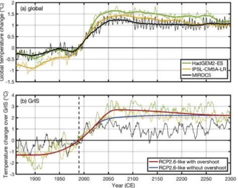
Frieler et al., 2017). We select RCP2.6 (Moss et al., 2010) because it is the lowest emission scenario considered within CMIP5 and roughly in line with the 1.5°C–2°C limit of global warming relative to pre-in- dustrial levels formulated in the Paris Agreement. The mean annual near-surface temperature change relative to 1990 over Greenland is shown inFig. 2. The results of HadGEM2-ES and IPSL-CM5A-LR both feature a significant Arctic amplification over Greenland (the tem- perature change over Greenland is larger than the global mean tem- perature change, which is also shown in the figure). By contrast, MIROC5 produces less pronounced warming over Greenland that is similar to the global mean warming. For this study, we construct two simplified scenarios for the surface temperature anomaly over Green- land (thick red and blue line inFig. 2b). These scenarios are designed as upper bounds of RCP2.6, based on the larger warming trends produced by the GCMs HadGEM2-ES and IPSL-CM5A-LR. We construct a sim- plified RCP2.6 scenario with overshoot as a spline interpolation of a few target points. These targets points were set in order to represent pro- nounced warming in the middle of this century and a decline after- wards. For a scenario without overshoot, we adjusted the query point in the middle of this century to suppress the overshoot. Both scenarios end at the same temperature rise over Greenland by 2300. Additionally, we define a control run to capture the drift of our two ice sheet models.
This leads to the following three experiments:
•
Constant climate control run: The climate is held steady to the re- ference temperature (year 1990).•
RCP2.6-like with overshoot: Relative to 1990, this produces an in- terim overshoot of 2.7°C in the second half of the 21st century, and a final warming of 2.2°C by 2300.•
RCP2.6-like without overshoot: Like above, but the interim over- shoot has been eliminated. Thus, warming proceeds monotonically until 2300 and settles at 2.2°C.Note that the RCP2.6-like warming trends are applied over the whole ice sheet, without spatial variations and interannual/decadal variability. The simulations with SICOPOLIS and ISSM start at 1990, indicated by the red dot inFig. 2b. Initial conditions are provided by the spin-up, as described in Sect. 3.1 for SICOPOLIS and in Sect. 3.2 for ISSM. The simulations proceed until 2300, using the same time steps as
reported in these sections. For the precipitation change, conversion to solid precipitation and surface melting (PDD), the same assumptions as for the paleoclimatic spin-up are made (see Sect. 3.1).
For the SICOPOLIS runs, the ice discharge parameterization used for the spin-up sequence and the SMB correction prescribed for the last 1 ka (step 4 of the spin-up sequence) are also employed for the future cli- mate runs. For the ISSM runs, an ice discharge parametrization it is not needed because of the higher horizontal resolution near the ice margin that captures ice discharge into the ocean directly with sufficient ac- curacy. Further, rather than using the SMB correction from SICOPOLIS, we derive a different correction by carrying out an auxiliary constant climate run over a single year. The resulting ice thickness imbalance,
H t/ , is used as the SMB correction for ISSM.
The SMB corrections applied to SICOPOLIS and ISSM are 221 Gt a−1 and 188 Gt a−1, respectively. As the spatially integrated values are positive, mass is added to the total mass balance budget M=SMB−BMB−D+SMBcorr. Here, SMB and BMB are the spatially integrated surface and basal mass balance, respectively, and D the ice discharge to the ocean. In doing so, the total mass balance budget is closed in the control run for both models (compareFig. 8). The SMB corrections occur predominantly at marine-terminating ice margins and ice streams. For these locations, the corrections can be considered as an additional ice thinning or thickening due to dynamic discharge that is not intrinsically simulated.
Due to the different complexity, the computational demand of the two models is vastly different. For SICOPOLIS, the future climate runs require ∼1 h each on a single CPU (Intel Xeon E5-2697 v2, 2.7 GHz). By contrast, an ISSM future climate run requires ∼48 h on 720 CPUs (Intel Xeon Broadwell E5-2697 v4, 2.3 GHz).
4. Results and discussion 4.1. Spin-up
The evolution of the ice volume and area for the 134 ka spin-up simulation is shown in Fig. 3. During the Eemian, a pronounced minimum occurs with an ice volume ∼2 m SLE less than today's.
During most of the last (Weichselian) glacial period, the entire available land area is glaciated, and on average ∼1 m SLE more ice than today is stored in the ice sheet. Aftert= 9 ka, both the volume and the area
drop rapidly, which is due to the nudging towards the (slightly smoothed) present-day topography that starts at this time with run (3) (see Sect. 3.1).
For the final timet=0(corresponding to the year 1990), the spin- up produces a Greenland ice sheet with a volume of
= ×
Vsim 3.004 10 km6 3 (7.43 m SLE) and an area of
= ×
Asim 1.856 10 km6 2. These numbers agree very well with their ob- served counterparts,Vobs=2.96×10 km6 3(7.36 m SLE) (Bamber et al., 2013) and Aobs=1.801×10 km6 2 (Kargel et al., 2012). The good agreement is mainly a consequence of the applied SMB correction in the spin-up run (4).
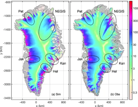
Fig. 4depicts the simulated and observed present-day surface ve- locities. The simulation reproduces the general pattern very well, in particular, the slow-flowing “backbone” of the ice sheet and the orga- nization of the coastward flow in distinct drainage systems. Despite the use of the SIA, even most of the fast-flowing ice streams and outlet glaciers are resolved reasonably well by the simulation (see alsoGreve and Herzfeld, 2013). Specifically, this holds true for Jakobshavn Ice Stream, Helheim and Kangerdlussuaq glaciers. The agreement is not so good for Petermann Glacier, likely because the real-world glacier has a floating ice tongue that cannot be modelled by our grounded-ice-only dynamics. A similar problem appears at the mouth of the North-East Fig. 2.Mean-annual near-surface temperature change re- lative to 1980–2000: (a) global, (b) over Greenland.
Simulated with the three GCMs HadGEM2-ES (green), IPSL- CM5A-LR (yellow) and MIROC5 (black) from the ISIMIP2b project (Frieler et al., 2017). The thick lines in the upper panel (a) is a 30-year moving mean. Simplified scenarios for Greenland: RCP2.6-like with (thick red) and without over- shoot (thick blue); 1990 level indicated by vertical dashed line.
Fig. 3.Ice volume (blue, in m SLE = metres of sea-level equivalent) and area (red) for the spin-up simulation with SICOPOLIS: Run (1) beforet= 9 ka, run (3) betweent= 9and −1 ka, run (4) aftert= 1 ka. Dashed lines indicate present-day (t=0) values. (For interpretation of the references to colour in this figure legend, the reader is referred to the Web version of this article.)
Greenland Ice Stream (NEGIS), where the ice tongues of the two northern outlet glaciers (79° North Glacier and Zachariæ Ice Stream) are cut off by the simulation, whereas the grounded southern outlet glacier (Storstrømmen Glacier) is reproduced well. A notable dis- crepancy is that the distinctive inland extent of the NEGIS is less pro- nounced in the simulation. This is likely due to unmodelled processes, possibly the presence of a geothermal heat flux anomaly at the onset of the NEGIS (Fahnestock et al., 2001) or sliding influenced by basal hy- drology (e.g.,Beyer et al., 2017;Calov et al., 2018), and deserves fur- ther attention in future studies.
4.2. Future projections 4.2.1. Control experiment
In the constant climate control experiment, we investigate the model response in the absence of additional forcing. The simulated sea level contribution over time is shown inFig. 5(dash-dotted lines). For both models, the drift is very small: during the 310 years integration time, SICOPOLIS/SIA gains mass equivalent to ∼2 mm SLE, while ISSM/HO gains ∼4 mm SLE.
Simulated surface velocities and basal temperatures for SICOPOLIS/SIA and ISSM/HO for the year 2300 are shown inFig. 6a, d
andFig. 6b,e, respectively, and the corresponding differences between the models in Fig. 6c,f. The simulated surface velocities of the two models reveal in general a similar pattern. However, ISSM/HO tends to produce lower velocities all around the ice margin for the outlet glaciers (Fig. 6c), most notably in the south and east. Exceptions are the NEGIS as well as Petermann and Humboldt glaciers, for which the ISSM ve- locities are still lower directly near the termini, but clearly larger fur- ther upstream.
The basal temperatures produced by both models (Fig. 6d and e) reveal a very similar pattern, with extended areas at the pressure melting point. Generally, ISSM/HO tends to produce a slight warming of initially cold ice in the interior of the ice sheet (blueish areas in Fig. 6f), while at the margins the ice base tends to become colder with ISSM/HO (reddish areas inFig. 6f), and locally even drops below the pressure melting point.
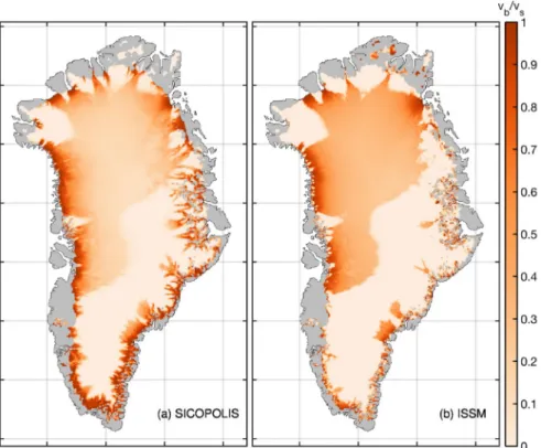
We relate the somewhat differing results for the velocity and tem- perature fields mainly to the different grid resolution and the imposed ice dynamics approximation of the two models. The representation of fast- flowing ice streams and outlet glaciers benefits from the unstructured grid of ISSM/HO, leading to higher resolution in narrow troughs, and the consideration of lateral drag by horizontal shear stresses that are neglected in the SIA. As a consequence, the fast flow of outlet glaciers is more re- stricted in ISSM/HO, while SICOPOLIS/SIA tends to overestimate their flow due to missing lateral drag. Additionally, the slip ratio (ratio of basal to surface velocity),v vb/s, reflects the different dynamical behaviour of both models (Fig. 7). SICOPOLIS/SIA reveals more sliding compared to ISSM/HO, particularly at the southern margins. We attribute this to the basal shear stress, which is always equal to the full driving stress in the SIA, but generally lower for fast-flowing ice in the HO. The consequence is that the SICOPOLIS/SIA solution has higher basal stresses, and thus more basal sliding, than ISSM/HO. The generally lower velocities produced by ISSM/HO near the ice margin lead to reduced heat production (due to volumetric strain heating and basal frictional heating). This process ex- plains the lower temperatures near the margin, which reduce the basal sliding even more via its strong temperature dependence due to the ex- ponentially decaying sub-melt-sliding term in Eq.(1).
Fig. 8depicts the components of the total mass balance of the ice sheet (dash-dotted lines for the control experiment). In line with the small model drift of both models, the SMB, the basal mass balance (BMB) and the ice discharge in the surrounding ocean remain almost constant over the 310 Fig. 4.Surface velocity of the Greenland ice sheet. (a) Result from the spin-up simulation for the year 1990 si- mulated with SICOPOLIS. (b) Observed surface velocity (mean of 1995–2015) (Joughin et al., 2016,2018). Jak:
Jakobshavn Ice Stream, Hel: Helheim Glacier, Kan: Kan- gerdlussuaq Glacier, Pet: Petermann Glacier, NEGIS:
North-East Greenland Ice Stream.
Fig. 5.Sea level contribution of the Greenland ice sheet simulated with SICOPOLIS and ISSM for all conducted experiments.
years of model time. Whereas the SMB has almost the same value for the two models, the BMB of the SICOPOLIS control run is significantly larger than the ISSM counterpart. However, in absolute terms, the BMB is much smaller than the SMB and does not contribute much to the total mass balance. The lower flow velocities produced by ISSM/HO for most ice streams and outlet glaciers are reflected by the ice discharge, which is about 75 Gt a−1less for ISSM/HO than for SICOPOLIS/SIA.
4.2.2. RCP2.6-like projections
For the two simulations with RCP2.6-like forcing, the simulated mass losses (expressed as sea level contributions) as functions of time are shown inFig. 5(solid and dashed lines). No matter whether an interim overshoot takes place or not, both ISSM/HO and SICOPOLIS/SIA show first a strongly increasing and later an abating sea level contribution. By 2300, the projected range (relative to the respective control run) is
∼62–88 cm. There is no latency in the response of the ice sheet to the deviation of the two forcings from each other – the overshoot that sets in around 2025 has an almost immediate effect on the mass loss.
For gaining an understanding of the drivers of mass loss, the
contributions of SMB, BMB and ice discharge to the total mass balance of the ice sheet are presented inFig. 8(solid and dashed lines for the RCP2.6-like scenarios). As expected, the SMB is immediately affected by the temperature rise. The difference between the scenarios with and without overshoot is here most striking: while no overshoot leads to a monotonic approach to the new, smaller SMB level with only a minor further decrease after 2150, the overshoot scenario clearly produces an interim minimum around 2070, more than 100 Gt a−1lower. Beyond that, the SMB for the overshoot scenario recovers partly and approaches that of the no-overshoot scenario at the end of the 23rd century. The difference between SICOPOLIS/SIA and ISSM/HO is quite substantial, reaching for both scenarios values of more than 50 Gt a−1as warming progresses.
The BMB is largely unaffected by the changes in atmospheric for- cing. This behaviour is as expected because changes in the basal thermal conditions can only occur with a significant lag due to the large thermal inertia of the system. The ice discharge does not react to the forcing as instantaneously as the SMB and exhibits more than a decade of latency. For both models and both scenarios, it falls below the Fig. 6.(a,b) Surface velocity and (d,e) basal temperature relative to pressure melting of the Greenland ice sheet for the constant climate control experiment, simulated with (a,d) SICOPOLIS/SIA and (b,e) ISSM/HO for the year 2300. (c,f) Difference between SICOPOLIS/SIA and ISSM/HO (the results on the structured SICOPOLIS grid were interpolated to the unstructured ISSM grid for comparison).
respective 1990 levels. Contrary to the SMB, for the overshoot sce- narios, the ice discharge does not show a pronounced minimum; rather, it decreases essentially monotonically throughout the model time.
The difference between the ISSM/HO and the SICOPOLIS/SIA results is pronounced, in that the discharge drop is much larger for SICOPOLIS/SIA. This is likely a consequence of the different treatments in the two models: while ISSM/HO computes discharge from outlet glaciers into the surrounding ocean directly on the high-resolution grid, SICOPOLIS/SIA employs an ice discharge parameterization to capture sub-grid-scale discharge (see Sect. 3.3).
Fig. 9displays the changes in ice surface velocities and thicknesses as 2300–1990 differences for the RCP2.6-like forcing with overshoot. (The corresponding differences for the no-overshoot case are somewhat smaller, but show similar spatial patterns, so they are not shown here.) The response of the velocities (Fig. 9a and b) to warming is notably different in both models. Along the west coast up to the north, SICOPOLIS/SIA shows a deceleration at glacier termini. Further up- stream, in the south and south-west acceleration is predominant. With ISSM/HO, we find a similar pattern in some outlet glaciers; however, along the north-western coast individual glaciers experience entirely acceleration or deceleration. In this area, acceleration patterns extend far inland, which we attribute to the resolution, as glacier valleys in this area are quite narrow and thus not resolved well by the coarser grid of SICOPOLIS. The region of the Jakobshavn Ice Stream shows a more complex pattern for SICOPOLIS/SIA than for ISSM/HO, featuring an acceleration that reaches much further upstream. Here, the differences between the models are certainly affected by the treatment of lateral shear, as HO is supposed to concentrate acceleration inside the main trunks by forming shear zones. With narrow glacier valleys being present in the south-east, the separation between glaciers is better represented by unstructured grids and, consequently, ISSM/HO leads to acceleration concentrated in narrow main flow troughs with high magnitude. At some locations, we observe for the ISSM/HO simulations deceleration at gla- cier termini, while further upstream acceleration is observed. This is due to a flattening at the termini, which goes along with deceleration, while steeper slopes propagate further upstream, leading to acceleration there.
In the north and north-east, at locations where floating ice tongues are present in today's observed ice sheet that are missing in the simu- lation results, both models respond differently. For the Petermann and Humboldt glaciers, SICOPOLIS/SIA responds with deceleration, while ISSM/HO facilitates the formation of shear margins. The NEGIS outlet glaciers show a distinct pattern: for ISSM/HO, 79° North Glacier ac- celerates, while Zachariæ Ice Stream slows down. For both models, Storstrømmen Glacier accelerates strongly.
Despite these differences in the detailed, dynamic response, both models show a similar pattern of ice thickness change: extensive mar- ginal thinning and moderate thickening in the interior. In general, for ISSM/HO, thinning reaches farther inland in the north and north-west, while SICOPOLIS/SIA produces a wider extent of thinning in the south- west. Specifically, ISSM/HO produces more mass loss at the margins of the northern basins (e.g., NEGIS), while SICOPOLIS/SIA produces a larger mass loss in the Jakobshavn area. The interaction of the SMB with ice dynamics can explain the different behaviour as the relative importance of outlet glacier dynamics decreases with increasing surface melt. Increased ice discharge causes dynamic thinning further up- stream, lowering the ice surface and thus intensifying surface melting due to the associated warming. In turn, surface melting competes with the discharge increase by removing ice before it reaches the marine margin. However, the level of interaction between SMB change and ice flow is very complex as the processes are mutually competitive. ISSM/
HO exhibits a localized thickening in the north of Jakobshavn Ice Stream. On closer inspection, this originates from a shear margin that becomes more pronounced over time in ISSM/HO, with a deceleration outside the main fast-flow area, which piles up ice. In the south-east, ISSM/HO produces thickening as a continuous band along the glacier margins, even though the acceleration is concentrated in valleys. We infer this pattern to be due to the dynamic feedback of the SMB, which distributes the thinning laterally. ISSM/HO exhibits thickening just upstream of the extent of acceleration.
As we have seen above, for both surface velocity and ice thickness changes, using an unstructured grid and including higher-order stresses is advantageous for capturing the detailed response of the Greenland ice Fig. 7.Slip ratio (ratio of basal to surface velocity),v vb/s, of the Greenland ice sheet for the constant climate control experiment, simulated with (a) SICOPOLIS/SIA and (b) ISSM/HO for the year 2300.
sheet to warming scenarios. On the one hand, the general patterns of ice thickness change produced by our two models agree well, and a clear pro of the simpler approach using the SIA and the structured grid is the drastically reduced computational demand. However, on the other hand, the differences between the models accumulate to notable dif- ferences in sea level contributions. In our simulations, the predicted contributions of the ice sheet decay to sea level rise differ by about 18%, which is not a catastrophic disagreement, but still considerable.
Our approach only allowed assessing the uncertainties arising from the different ice dynamics approximations and the different grids jointly. This is a typical situation often encountered in model inter- comparison studies like, e.g., initMIP-Greenland (Goelzer et al., 2018):
models with structured grids employing the SIA or an SIA/SSA hybrid vs. models with unstructured grids employing HO or FS dynamics.
Other studies also aimed at assessing the differences arising from model physics and discretization in climate forcing experiments.Seddik et al.
(2012) reported that the FS model Elmer/Ice, using an unstructured grid, produces ∼61% less mass loss for the Greenland ice sheet after 100 years than SICOPOLIS used in a similar configuration like in our study. By contrast, we found ISSM/HO to be ∼18% more sensitive (larger mass loss) to climate forcing than SICOPOLIS. Seddik et al.
(2017)separated the effect of model physics from discretization and implementation details by applying the same model Elmer/Ice in FS mode and in SIA mode to the Shirase drainage basin of the Antarctic ice sheet. They found that the change in ice volume for a climate forcing experiment is nearly independent of the model physics, which high- lights the effects of discretization and implementation. However, the
latter finding is of limited relevance in our context: in contrast to the Greenland ice sheet, the sensitivity of the Antarctic ice sheet to direct climate forcing is generally small, whereas it is more vulnerable to ocean-induced sub-ice-shelf melting (e.g.,Bindschadler et al., 2013).
5. Summary and conclusion
The ice flow models ISSM and SICOPOLIS were applied to the entire Greenland ice sheet. SICOPOLIS employed the shallow ice approxima- tion (SIA) on a structured grid with 5 km resolution, while ISSM used a higher-order approximation (HO) of the Stokes equation on an un- structured grid with a resolution varying from 1 to 20 km. Starting from a paleoclimatic spin-up produced by SICOPOLIS, we forced the models with two different, simplified RCP2.6-like warming scenarios derived from the output of climate models, which are in line with the limit of global warming negotiated for the Paris Agreement.
For the RCP2.6-like scenario with interim overshoot, by the year 2300, we computed a sea level contribution from the Greenland ice sheet of ∼88 mm with ISSM/HO and ∼73 mm with SICOPOLIS/SIA.
The no-overshoot scenario led to lower numbers, ∼75 mm with ISSM/
HO and ∼62 mm with SICOPOLIS/SIA. (All numbers are given relative to the respective constant climate control run.) Thus, for both models, we have a ∼18% larger contribution due to the overshoot. Keeping in mind that the amount of overshoot assumed here is only moderate, this result highlights the potential of an overshoot to enhance mass loss of ice sheets.
Compared to the impact of more severe warming scenarios on the Fig. 8.Components of the total mass balance for all conducted experiments. (a) Surface mass balance (SMB). Positive values represent accumulation and negative values ablation. (b) Basal mass balance (BMB). Positive values represent basal melting. (c) Discharge into the ocean.
Greenland ice sheet, the above range of mass loss (62–88 mm SLE after 310 years) is modest. One of the experiments of the recent initMIP- Greenland initiative consisted of prescribing a schematic SMB anomaly that corresponds to an upper-end climate change scenario like RCP8.5.
For this experiment (“asmb”), the simulated range of mass loss across all participating models after only 100 years was 75–290 mm SLE (87–172 mm SLE for the four different contributions using ISSM and the two different contributions using SICOPOLIS) (Goelzer et al., 2018).
This demonstrates that meeting the targets of the Paris Agreement can significantly reduce the risks and impacts of climate change.
However, neither our main focus, nor that of initMIP-Greenland, was providing detailed projections; this will be deferred to future work within the Ice Sheet Model Intercomparison Project for CMIP6 (ISMIP6;Nowicki
et al., 2016). Rather, we attempted to quantify the effects of different model physics, numerical techniques and implementation on projections of future mass loss, keeping all other settings of the two models as similar as possible. For both the RCP2.6-like scenario with and without interim overshoot, we found that ISSM/HO produces a bit more than 10 mm SLE additional mass loss compared to SICOPOLIS/SIA, while the general trends are similar in both models. We attributed the larger sensitivity of ISSM/HO to a larger discharge into the surrounding ocean and a lower SMB. These two effects are connected because ISSM/HO produces more acceleration of narrow outlet glaciers, leading to more discharge and dynamic thinning, which, in turn, reduces the SMB. Due to the higher resolution of the un- structured grid of ISSM near the ice margin and the HO dynamics, we assess the ISSM results to be the more realistic ones. The different Fig. 9.(a,b) Surface velocity changes and (c,d) ice thickness changes of the Greenland ice sheet for 2300–1990 and the RCP2.6-like scenario with overshoot, simulated with (a,c) SICOPOLIS and (b,d) ISSM.
sensitivities of our two models exemplify that, besides further efforts re- quired to create realistic climate forcings, significant uncertainties in sea level projections arise directly and indirectly – via feedbacks on the SMB – from model physics and grid resolution.
Acknowledgments
We thank Ayako Abe-Ouchi (Univ. Tokyo) for helpful discussions about the different GCM results and the ISSM team, in particular Mathieu Morlighem (Univ. California Irvine), for their support. Further, we thank the anonymous reviewer for constructive remarks and sug- gestions that helped to improve the manuscript.
Martin Rückamp was funded by the Helmholtz Climate Initiative REKLIM (Regional Climate Change), a joint research project of the Helmholtz Association of German Research Centres (HGF). Angelika Humbert acknowledges funding of this work by BMBF under grant EP- GrIS (01LS1603A). Ralf Greve and Martin Rückamp were supported by Japan Society for the Promotion of Science (JSPS) KAKENHI grant number JP16H02224. Ralf Greve was supported by JSPS KAKENHI grant number JP17H06104, and by the Japanese Ministry of Education, Culture, Sports, Science and Technology (MEXT) through the Arctic Challenge for Sustainability (ArCS) project.
References
Aschwanden, A., Aalgeirsdóttir, G., Khroulev, C., 2013. Hindcasting to measure ice sheet model sensitivity to initial states. Cryosphere 7 (4), 1083–1093.
Aschwanden, A., Fahnestock, M.A., Truffer, M., 2016. Complex Greenland outlet glacier flow captured. Nat. Commun. 7, 10524.
Bales, R.C., Guo, Q., Shen, D., McConnell, J.R., Du, G., Burkhart, J.F., Spikes, V.B., Hanna, E., Cappelen, J., 2009. Annual accumulation for Greenland updated using ice core data developed during 2000–2006 and analysis of daily coastal meteorological data.
J. Geophys. Res. Atmos. 114 (D6), D06116.
Bamber, J.L., Griggs, J.A., Hurkmans, R.T.W.L., Dowdeswell, J.A., Gogineni, S.P., Howat, I., Mouginot, J., Paden, J., Palmer, S., Rignot, E., Steinhage, D., 2013. A new bed elevation dataset for Greenland. Cryosphere 7 (2), 499–510.
Bernales, J., Rogozhina, I., Greve, R., Thomas, M., 2017. Comparison of hybrid schemes for the combination of shallow approximations in numerical simulations of the Antarctic Ice Sheet. Cryosphere 11 (1), 247–265.
Beyer, S., Kleiner, T., Aizinger, V., Rückamp, M., Humbert, A., 2017. A confined-un- confined aquifer model for subglacial hydrology and its application to the North East Greenland Ice Stream. Cryosphere Discuss.https://doi.org/10.5194/tc–2017–221.
Bindschadler, R.A., Nowicki, S., Abe-Ouchi, A., Aschwanden, A., Choi, H., Fastook, J., Granzow, G., Greve, R., Gutowski, G., Herzfeld, U.C., Jackson, C., Johnson, J., Khroulev, C., Levermann, A., Lipscomb, W.H., Martin, M.A., Morlighem, M., Parizek, B.R., Pollard, D., Price, S.F., Ren, D., Saito, F., Sato, T., Seddik, H., Seroussi, H., Takahashi, K., Walker, R., Wang, W.L., 2013. Ice-sheet model sensitivities to en- vironmental forcing and their use in projecting future sea level (the SeaRISE project).
J. Glaciol. 59 (214), 195–224.
Blatter, H., 1995. Velocity and stress fields in grounded glaciers: a simple algorithm for including deviatoric stress gradients. J. Glaciol. 41 (138), 333–344.
Bondzio, J.H., Morlighem, M., Seroussi, H., Kleiner, T., Rückamp, M., Mouginot, J., Moon, T., Larour, E.Y., Humbert, A., 2017. The mechanisms behind Jakobshavn Isbræ’s acceleration and mass loss: a 3-D thermomechanical model study. Geophys. Res. Lett.
44 (12), 6252–6260.
Calov, R., Beyer, S., Greve, R., Beckmann, J., Willeit, M., Kleiner, T., Rückamp, M., Humbert, A., Ganopolski, A., 2018. Simulation of the future sea level contribution of Greenland with a new glacial system model. Cryosphere 12 (10), 3097–3121.
Calov, R., Greve, R., 2005. A semi-analytical solution for the positive degree-day model with stochastic temperature variations. J. Glaciol. 51 (172), 173–175.
Calov, R., Robinson, A., Perrette, M., Ganopolski, A., 2015. Simulating the Greenland ice sheet under present-day and palaeo constraints including a new discharge para- meterization. Cryosphere 9 (1), 179–196.
Cuffey, K.M., Paterson, W.S.B., 2010. The Physics of Glaciers, fourth ed. Elsevier, Amsterdam, The Netherlands etc.
Fahnestock, M., Abdalati, W., Joughin, I., Brozena, J., Gogineni, P., 2001. High geo- thermal heat flow, basal melt, and the origin of rapid ice flow in central Greenland.
Science 294 (5550), 2338–2342.
Fausto, R.S., Ahlstrøm, A.P., van As, D., Bøggild, C.E., Johnsen, S.J., 2009. A new present- day temperature parameterization for Greenland. J. Glaciol. 55 (189), 95–105.
Frieler, K., Lange, S., Piontek, F., Reyer, C.P.O., Schewe, J., Warszawski, L., Zhao, F., Chini, L., Denvil, S., Emanuel, K., Geiger, T., Halladay, K., Hurtt, G., Mengel, M., Murakami, D., Ostberg, S., Popp, A., Riva, R., Stevanovic, M., Suzuki, T., Volkholz, J., Burke, E., Ciais, P., Ebi, K., Eddy, T.D., Elliott, J., Galbraith, E., Gosling, S.N., Hattermann, F., Hickler, T., Hinkel, J., Hof, C., Huber, V., Jägermeyr, J., Krysanova, V., Marcé, R., Müller Schmied, H., Mouratiadou, I., Pierson, D., Tittensor, D.P., Vautard, R., van Vliet, M., Biber, M.F., Betts, R.A., Bodirsky, B.L., Deryng, D., Frolking, S., Jones, C.D., Lotze, H.K., Lotze-Campen, H., Sahajpal, R., Thonicke, K.,
Tian, H., Yamagata, Y., 2017. Assessing the impacts of 1.5°C global warming – si- mulation protocol of the inter-sectoral impact model intercomparison project (ISIMIP2b). Geosci. Model Dev. (GMD) 10 (12), 4321–4345.
Fürst, J.J., Goelzer, H., Huybrechts, P., 2013. Effect of higher-order stress gradients on the centennial mass evolution of the Greenland ice sheet. Cryosphere 7 (1), 183–199.
Gillet-Chaulet, F., Gagliardini, O., Seddik, H., Nodet, M., Durand, G., Ritz, C., Zwinger, T., Greve, R., Vaughan, D.G., 2012. Greenland ice sheet contribution to sea-level rise from a new-generation ice-sheet model. Cryosphere 6 (6), 1561–1576.
Goelzer, H., Nowicki, S., Edwards, T., Beckley, M., Abe-Ouchi, A., Aschwanden, A., Calov, R., Gagliardini, O., Gillet-Chaulet, F., Golledge, N.R., Gregory, J., Greve, R., Humbert, A., Huybrechts, P., Kennedy, J.H., Larour, E., Lipscomb, W.H., Le clec’h, S., Lee, V., Morlighem, M., Pattyn, F., Payne, A.J., Rodehacke, C., Rückamp, M., Saito, F., Schlegel, N., Seroussi, H., Shepherd, A., Sun, S., van de Wal, R., Ziemen, F.A., 2018.
Design and results of the ice sheet model initialisation experiments initMIP- Greenland: an ISMIP6 intercomparison. Cryosphere 12 (4), 1433–1460.
Greve, R., 1997. Application of a polythermal three-dimensional ice sheet model to the Greenland ice sheet: response to steady-state and transient climate scenarios. J. Clim.
10 (5), 901–918.
Greve, R., 2019. Geothermal heat flux distribution for the Greenland ice sheet, derived by combining a global representation and information from deep ice cores. Polar Data J.
3, 22–36.
Greve, R., Blatter, H., 2009. Dynamics of Ice Sheets and Glaciers. Springer, Berlin, Germany etc.
Greve, R., Blatter, H., 2016. Comparison of thermodynamics solvers in the polythermal ice sheet model SICOPOLIS. Polar Sci. 10 (1), 11–23.
Greve, R., Herzfeld, U.C., 2013. Resolution of ice streams and outlet glaciers in large-scale simulations of the Greenland ice sheet. Ann. Glaciol. 54 (63), 209–220.
Hutter, K., 1983. Theoretical Glaciology; Material Science of Ice and the Mechanics of Glaciers and Ice Sheets. D. Reidel Publishing Company, Dordrecht, The Netherlands.
Huybrechts, P., 2002. Sea-level changes at the LGM from ice-dynamic reconstructions of the Greenland and Antarctic ice sheets during the glacial cycles. Quat. Sci. Rev. 21 (1–3), 203–231.
Huybrechts, P., de Wolde, J., 1999. The dynamic response of the Antarctic and Greenland ice sheets to multiple-century climatic warming. J. Clim. 12 (8), 2169–2188.
Imbrie, J., Hays, J.D., Martinson, D.G., McIntyre, A., Mix, A.C., Morley, J.J., Pisias, N.G., Prell, W.L., Shackleton, N.J., 1984. The orbital theory of Pleistocene climate: support from a revised chronology of the marine 18O record. In: Berger, A., Imbrie, J., Hays, J., Kukla, G., Saltzman, B. (Eds.), Milankovitch and Climate, Part I. Reidel, Dordrecht, The Netherlands, pp. 269–305 NATO ASI Series C: Mathematical and Physical Sciences 126.
IPCC, 2018. Special report on global warming of 1.5°C (SR15).http://www.ipcc.ch/
report/sr15/, Accessed date: November 2018.
Joughin, I., Smith, B.E., Howat, I.M., 2018. A complete map of Greenland ice velocity derived from satellite data collected over 20 years. J. Glaciol. 64 (243), 1–11.
Joughin, I., Smith, B.E., Howat, I.M., Scambos, T., 2016. MEaSUREs Multi-year Greenland Ice Sheet Velocity Mosaic, Version 1. Dataset, NASA National Snow and Ice Data Center Distributed Active Archive Center. Boulder, Colorado, USA. http://doi.org/
10.5067/QUA5Q9SVMSJG.
Kargel, J.S., Ahlstrøm, A.P., Alley, R.B., Bamber, J.L., Benham, T.J., Box, J.E., Chen, C., Christoffersen, P., Citterio, M., Cogley, J.G., Jiskoot, H., Leonard, G.J., Morin, P., Scambos, T., Sheldon, T., Willis, I., 2012. Brief communication: Greenland's shrinking ice cover: “fast times” but not that fast. Cryosphere 6 (3), 533–537.
Kleiner, T., Rückamp, M., Bondzio, J.H., Humbert, A., 2015. Enthalpy benchmark ex- periments for numerical ice sheet models. Cryosphere 9 (1), 217–228.
Kobashi, T., Kawamura, K., Severinghaus, J.P., Barnola, J.-M., Nakaegawa, T., Vinther, B.M., Johnsen, S.J., Box, J.E., 2011. High variability of Greenland surface tempera- ture over the past 4000 years estimated from trapped air in an ice core. Geophys. Res.
Lett. 38 (21), L21501.
Larour, E., Seroussi, H., Morlighem, M., Rignot, E., 2012. Continental scale, high order, high spatial resolution, ice sheet modeling using the Ice Sheet System Model (ISSM).
J. Geophys. Res. Earth Surf. 117 (F1), F01022.
Le Meur, E., Huybrechts, P., 1996. A comparison of different ways of dealing with iso- stasy: examples from modelling the Antarctic ice sheet during the last glacial cycle.
Ann. Glaciol. 23, 309–317.
Lliboutry, L., Duval, P., 1985. Various isotropic and anisotropic ices found in glaciers and polar ice caps and their corresponding rheologies. Ann. Geophys. 3 (2), 207–224.
MacAyeal, D.R., 1989. Large-scale ice flow over a viscous basal sediment: theory and application to ice stream B, Antarctica. J. Geophys. Res. Solid Earth 94 (B4), 4071–4087.
Morland, L.W., 1984. Thermomechanical balances of ice sheet flows. Geophys. Astrophys.
Fluid Dynam. 29, 237–266.
Morland, L.W., 1987. Unconfined ice-shelf flow. In: van der Veen, C.J., Oerlemans, J.
(Eds.), Dynamics of the West Antarctic Ice Sheet. D. Reidel Publishing Company, Dordrecht, The Netherlands, pp. 99–116.
Morlighem, M., Williams, C.N., Rignot, E., An, L., Arndt, J.E., Bamber, J.L., Catania, G., Chauché, N., Dowdeswell, J.A., Dorschel, B., Fenty, I., Hogan, K., Howat, I., Hubbard, A., Jakobsson, M., Jordan, T.M., Kjeldsen, K.K., Millan, R., Mayer, L., Mouginot, J., Noël, B.P.Y., O'Cofaigh, C., Palmer, S., Rysgaard, S., Seroussi, H., Siegert, M.J., Slabon, P., Straneo, F., van den Broeke, M.R., Weinrebe, W., Wood, M., Zinglersen, K.B., 2017. BedMachine v3: complete bed topography and ocean bathymetry map- ping of Greenland from multibeam echo sounding combined with mass conservation.
Geophys. Res. Lett. 44 (21), 11051–11061.
Moss, R.H., Edmonds, J.A., Hibbard, K.A., Manning, M.R., Rose, S.K., van Vuuren, D.P., Carter, T.R., Emori, S., Kainuma, M., Kram, T., Meehl, G.A., Mitchell, J.F.B., Nakicenovic, N., Riahi, K., Smith, S.J., Stouffer, R.J., Thomson, A.M., Weyant, J.P., Wilbanks, T.J., 2010. The next generation of scenarios for climate change research
and assessment. Nature 463 (7282), 747–756.
Nerem, R.S., Beckley, B.D., Fasullo, J.T., Hamlington, B.D., Masters, D., Mitchum, G.T., 2018. Climate-change-driven accelerated sea-level rise detected in the altimeter era.
P. Natl. Acad. Sci. 115 (9), 2022–2025.
Nielsen, L.T., Aalgeirsdóttir, G., Gkinis, V., Nuterman, R., Hvidberg, C.S., 2018. The effect of a Holocene climatic optimum on the evolution of the Greenland ice sheet during the last 10 kyr. J. Glaciol. 64 (245), 477–488.
North Greenland Ice Core Project members, 2004. High-resolution record of Northern Hemisphere climate extending into the last interglacial period. Nature 431 (7005), 147–151.
Nowicki, S., Bindschadler, R.A., Abe-Ouchi, A., Aschwanden, A., Bueler, E., Choi, H., Fastook, J., Granzow, G., Greve, R., Gutowski, G., Herzfeld, U., Jackson, C., Johnson, J., Khroulev, C., Larour, E., Levermann, A., Lipscomb, W.H., Martin, M.A., Morlighem, M., Parizek, B.R., Pollard, D., Price, S.F., Ren, D., Rignot, E., Saito, F., Sato, T., Seddik, H., Seroussi, H., Takahashi, K., Walker, R., Wang, W.L., 2013.
Insights into spatial sensitivities of ice mass response to environmental change from the SeaRISE ice sheet modeling project II: Greenland. J. Geophys. Res. Earth Surf. 118 (2), 1025–1044.
Nowicki, S.M.J., Payne, A., Larour, E., Seroussi, H., Goelzer, H., Lipscomb, W., Gregory, J., Abe-Ouchi, A., Shepherd, A., 2016. Ice sheet model intercomparison project (ISMIP6) contribution to CMIP6. Geosci. Model Dev. 9 (12), 4521–4545.
Pattyn, F., 2003. A new three-dimensional higher-order thermomechanical ice-sheet model: basic sensitivity, ice-stream development and ice flow across subglacial lakes.
J. Geophys. Res. Solid Earth 108 (B8), 2382.
Reeh, N., 1991. Parameterization of melt rate and surface temperature on the Greenland ice sheet. Polarforschung 59 (3), 113–128.
Rietbroek, R., Brunnabend, S.-E., Kusche, J., Schröter, J., Dahle, C., 2016. Revisiting the
contemporary sea-level budget on global and regional scales. P. Natl. Acad. Sci. 113 (6), 1504–1509.
Ritz, C., 1987. Time dependent boundary conditions for calculation of temperature fields in ice sheets. In: Waddington, E.D., Walder, J.S. (Eds.), The Physical Basis of Ice Sheet Modelling. IAHS Publication No. 170. IAHS Press, Wallingford, UK, pp. 207–216.
Robinson, A., Calov, R., Ganopolski, A., 2010. An efficient regional energy-moisture balance model for simulation of the Greenland Ice Sheet response to climate change.
Cryosphere 4 (2), 129–144.
Rogelj, J., Luderer, G., Pietzcker, R.C., Kriegler, E., Schaeffer, M., Krey, V., Riahi, K., 2015. Energy system transformations for limiting end-of-century warming to below 1.5°C. Nat. Clim. Change 5 (6), 519–527.
Sato, T., Greve, R., 2012. Sensitivity experiments for the Antarctic ice sheet with varied sub-ice-shelf melting rates. Ann. Glaciol. 53 (60), 221–228.
Seddik, H., Greve, R., Zwinger, T., Gillet-Chaulet, F., Gagliardini, O., 2012. Simulations of the Greenland ice sheet 100 years into the future with the full Stokes model Elmer/
Ice. J. Glaciol. 58 (209), 427–440.
Seddik, H., Greve, R., Zwinger, T., Sugiyama, S., 2017. Regional modeling of the Shirase drainage basin, East Antarctica: full Stokes vs. shallow ice dynamics. Cryosphere 11 (5), 2213–2229.
Seroussi, H., Morlighem, M., Larour, E., Rignot, E., Khazendar, A., 2014. Hydrostatic grounding line parameterization in ice sheet models. Cryosphere 8 (6), 2075–2087.
van den Broeke, M.R., Enderlin, E.M., Howat, I.M., Kuipers Munneke, P., Noël, B.P.Y., van de Berg, W.J., van Meijgaard, E., Wouters, B., 2016. On the recent contribution of the Greenland ice sheet to sea level change. Cryosphere 10 (5), 1933–1946.
Wolff, E.W., Chappellaz, J., Blunier, T., Rasmussen, S.O., Svensson, A., 2010. Millennial- scale variability during the last glacial: the ice core record. Quat. Sci. Rev. 29 (21–22), 2828–2838.