This project has received funding from the European Union’s Horizon 2020 research and innovation programme under grant agreement n

(1)

Last updated: 29 März 2019

This project has received funding from the European Union’s Horizon 2020 research and innovation programme under grant agreement n^o 633211.

Project AtlantOS – 633211

Deliverable number 3.18

Deliverable title Report on the observational potential of the TMAs

Description Assessment of the impact of upper-ocean measurements and of coherent integration of O2 measurements (as example for non-physical EOVs) for transports and fluxes in the Atlantic TMAs and synergies with the wider Atlantic Observing System. One workshop will be held to prepare the report and foster the cooperation on cross-TMA analyses.

Work Package number WP 3

Work Package title Enhancement of autonomous observing networks Lead beneficiary SAMS and Havstovan (MSS)

Lead authors Bee Berx, Stuart Cunningham

Contributors Wilken-Jon von Appen, Dariia Atamanchuk, Peter Brown, Neil Fraser, Johannes Hahn, Kerstin Jochumsen, Clare Johnson, Femke de Jong, Johannes Karstensen, Brian King, Matthias Lankhorst, Karin Margretha H. Larsen, Elaine McDonagh, Martin Moritz, Igor Yashayaev

Submission data 29 March 2019

Due date 31 December 2018 – extension to 31 March 2019 agreed with project office

Comments The deliverable was delayed due to the timing of instrument recovery from mooring deployment (summer 2018),

availability of PIs for a workshop in Edinburgh (eventually held in November 2018), and to ensure time to write a coherent report with input from across the community.

(2)

Stakeholder engagement relating to this task*

WHO are your most important stakeholders?

☐ Private company

If yes, is it an SME ☐ or a large company ☐?

☑ National governmental body

☑ International organization

☐ NGO

☐ others

Please give the name(s) of the stakeholder(s):

Research groups contributing to this report, other research organisations interested in deploying moored equipment WHERE is/are the company(ies) or

organization(s) from?

☑ Your own country

☐ Another country in the EU

☐ Another country outside the EU Please name the country(ies):

UK, Faroe Islands, Canada, Germany, the Netherlands, USA Is this deliverable a success story? If yes,

why?

If not, why?

☑ Yes, because planned tasks (a workshop and report discussing the potential for TMA sites to measure oxygen observations) have been achieved.

☐ No, because …..

Will this deliverable be used?

If yes, who will use it?

If not, why will it not be used?

☑ Yes, by the oceanographic community in bringing forward a standardized procedure for sustained oxygen observations in the ocean.

☐ No, because …..

NOTE: This information is being collected for the following purposes:

1. To make a list of all companies/organizations with which AtlantOS partners have had contact.

This is important to demonstrate the extent of industry and public-sector collaboration in the obs community. Please note that we will only publish one aggregated list of companies and not mention specific partnerships.

2. To better report success stories from the AtlantOS community on how observing delivers concrete value to society.

*For ideas about relations with stakeholders you are invited to consult D10.5 Best Practices in Stakeholder Engagement, Data Dissemination and Exploitation.

(3)

The observational potential of the Transport Mooring Arrays:

Assessment of the impact of upper-ocean

measurements and of coherent integration of O 2 measurements for transports and fluxes in the Atlantic TMAs and synergies with the

wider Atlantic Observing System

Barbara Berx, Marine Scotland Science, Aberdeen, UK

Stuart Cunningham, Scottish Association for Marine Science, Argyll, UK

Wilken-Jon von Appen, Alfred Wegener Institute Helmholtz Centre for Polar and Marine Research, Bremerhaven, Germany

Dariia Atamanchuk, Dalhousie University, Halifax, NS, Canada Peter Brown, National Oceanography Centre, Southampton, UK Neil Fraser, Scottish Association for Marine Science, Argyll, UK

Johannes Hahn, GEOMAR Helmholtz-Zentrum für Ozeanforschung Kiel, Germany

Kerstin Jochumsen, Federal Maritime and Hydrographic Agency (BSH), Hamburg, Germany Clare Johnson, Scottish Association for Marine Science, Argyll, UK

Femke de Jong, NIOZ Royal Netherlands Institute for Sea Research and Utrecht University, Texel, the Netherlands

Johannes Karstensen, GEOMAR Helmholtz-Zentrum für Ozeanforschung Kiel, Germany Brian King, National Oceanography Centre, Southampton, UK

Matthias Lankhorst, Scripps Institution of Oceanography, La Jolla, CA, USA

Karin Margretha H. Larsen, Havstovan - Faroe Marine Research Institute, Tórshavn, Faroe Islands Elaine McDonagh, National Oceanography Centre, Southampton, UK

Martin Moritz, Institute of Oceanography Hamburg (now at Federal Maritime and Hydrographic Agency), Hamburg, Germany

Igor Yashayaev, Bedford Institute for Oceanography, Halifax, NS, Canada

(4)

Executive Summary

Sustained observations of oxygen are critical to address some of the major societal challenges related to the impacts of climate change, such as anthropogenic carbon uptake and ocean deoxygenation. Oxygen is fundamental to sustaining the ocean’s ecosystems and plays an important role in global biogeochemical cycles.

Eight established Transport Mooring Arrays (TMAs) exist within the Atlantic Ocean. These provide an excellent platform to collect oxygen observations, due to a combination of their geographical location, regular ship visits and sustained activities. Within AtlantOS, several TMAs added oxygen sensors to the moorings, and some initial results are presented here.

At a workshop held in November 2018 in Edinburgh, and through consultation with the wider community, the addition of oxygen sensors to TMAs and the best practice for deployment, calibration and data processing are also presented here.

The continued efforts to fund these observations will allow oceanographers to help constrain global biogeochemical cycles – including those of Carbon and critical nutrients like Nitrogen; to better resolve ocean deoxygenation through high quality measurements; and to apply a mature technology regularly.

(5)

1 Introduction

Oxygen is fundamental to sustaining life in the ocean’s ecosystems, and plays a pivotal role in global biogeochemical cycles such as those of carbon (e.g. Bopp et al., 2002) and nutrients (e.g. Codispoti et al., 2001). Measurements of marine oxygen levels are critical to infer the activity of and changes in the

biological carbon system (e.g. Sarmiento and Gruber, 2006), and by extension they are a key component in helping to understand how the oceans absorb CO2 from the atmosphere (e.g. Sabin et al., 2004) and how it accumulates at depth over climatically-relevant timescales (Gruber et al., 2019). Moreover, dissolved oxygen can also be used to trace water masses and quantify ocean mixing (Karstensen et al., 2008) In recent years, observations show that areas of low oxygen are expanding and oxygen content is decreasing in many places (Schmidtko et al., 2017; Breitburg et al., 2018). Climate change impacts the ocean’s oxygen concentrations directly by reducing its solubility (the ability to hold oxygen decreases with increasing temperature) and indirectly by changing circulation and mixing (as increased stratification will reduce air-sea interaction), and oxygen respiration (Oschlies et al., 2018). The impact of ocean

deoxygenation on ecosystem productivity, fisheries and nitrous oxide production will have a large societal impact into the future (e.g. Codispoti et al., 2010; Gruber et al, 2011; Oschilies et al, 2018), . The Kiel Declaration (2018) has called for increased awareness to the issue of ocean deoxygenation, as well as mitigation measures and increased ocean observations of oxygen.

In addition to temperature and salinity measurements, oxygen is one of the oldest oceanographic

measurements. Winkler (1888) developed a chemical method to determine its concentration by titration, which remains almost unchanged. This allows for straightforward comparison of historic observations and for the creation of long time series data (e.g. Schmidtko et al., 2017; Breitburg et al., 2018), but the need for water sample collection and wet chemistry techniques is prohibitive of the high spatial and temporal resolution measurements modern oceanography requires. The development of electrochemical (Clark et al., 1953; Kanwisher, 1959) and optode (Tengberg et al., 2006) oxygen sensors has enabled oceanographers to collect oxygen observations at a similar spatial and temporal resolution to temperature and salinity.

These sensors are now regularly deployed on ship’s profiling CTDs (Uchida et al., 2010), on underway systems, profiling floats (Körtzinger et al., 2005) and oceanographic moorings (Brandt et al., 2015;

Karstensen et al., 2015). Optodes are explicitly useful for long-term measurements due to their stability during in-situ measurements. Other measurement techniques (Clark, Winkler) are not useful due to large drift behaviour (Clark) or simply being impracticable (Winkler). Within AtlantOS (WP 3.5), the PIRATA team have also used optodes for moored observations (Bourlès et al., 2018). Their explicit aim was to provide online oxygen observations and to enlarge the number of optode observations in PIRATA. In a more general perspective, (offline) optode observations within PIRATA exist already since 2009 (as shown in deliverable 3.9). To ensure high quality measurements, important considerations such as calibration, drift, response times and fouling remain.

Eulerian time series are coordinated in a global context by the OceanSITES observing network that is part of the Joint Technical Commission for Oceanography and Marine Meteorology (JCOMM) Observations

Programme Area (OPA) networks. OceanSITES collect, deliver and promote the use of high-quality data from long-term, high-frequency observations at fixed locations in the open ocean. The sites serve multiple purposes defined by the regional needs, but the three main objectives for operating the sites are:

(7)

 Transport mooring arrays (TMA) – these sites are often composed of an array of moorings that monitor ocean circulation (transport) and water mass characteristics (physical, biogeochemical, ecosystem); they also serve as calibration/validation (cal/val) sites for satellite altimetric transport comparisons;

 Air/sea flux reference sites – these sites have complex surface buoys accompanied by upper ocean instrumentation and serve as cal/val sites e.g. for satellite derived products related to weather and wave forecasting;

 Multidisciplinary Global Ocean Watch – these sites aim for long time series of properties across disciplines (physics, biology/ecosystem, biogeochemistry), and may also include cal/val

components for satellite ocean colour products.

One of the main drivers for OceanSITES time series is to provide both monitoring and process observations, with a temporal resolution from minutes to decades to detect, understand, and predict global physical, biogeochemical and ecosystem state and changes, including ocean warming, ocean carbon uptake/storage and acidification, but considering also the role of and impact on the ecosystem.

Since the mid-1990s, several Transport Mooring Arrays (TMAs) have been established to monitor the ocean transport pathways at key sections. Under AtlantOS, eight TMAs in the Atlantic Ocean (Figure 1) have been brought together. These TMAs traditionally measure temperature, salinity and currents, in order to

estimate ocean volume, heat and salt transports. In addition, to the observations already collected at these sites, these provide an opportunistic platform to measure other parameters, including oxygen. During the regular servicing of these moorings, ship-based measurements can be collected to calibrate or validate the observed parameters.

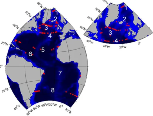
Figure 1. Overview map of the AtlantOS Transport Mooring Arrays (TMAs): 1. Fram Strait, 2. Greenland-Scotland Ridge (GSR), 3.

Overturning in the Subpolar North Atlantic Program (OSNAP), 4. North Atlantic Changes (NOAC), 5. Rapid Climate Change / Meridional Overturning Circulation Heat-flux Array / Western Boundary Time Series (RAPID/MOCHA/WBTS), 6. Meridional Overturning Variability Experiment (MOVE), 7. 11 S, 8. South Atlantic Meridional Overturning Circulation (SAMBA-SAMOC).

Oxygen is currently not measured at NOAC (4), 11S (7) and SAMBA-SAMOC (8). Figure courtesy of U. Schauer.

(8)

Oxygen observations at TMA sites can provide complementary information to those from ships and profiling floats. Simultaneous measurements of hydrography, velocity and oxygen allow the estimate of oxygen fluxes and to study driving mechanisms for oxygen variability, which is related to transport and water mass variability. The collection of these parameters at these oceanographically important regions will allow researchers to better understand oxygen variability and deoxygenation. Further, the regular servicing and ship-based surveys accompanying TMA deployments give an opportunity for good calibration data to supplement the high resolution data collection, thus providing better quality data at higher temporal resolution than ship surveys or float deployments can. In addition, sensors mounted on moorings instead of floats are also advantageous in boundary current regions: moored sensors remain in place in these fast moving (boundary) currents while profiling floats tend to converge in the slow moving interiors. Finally, oxygen sensors are now considered a mature technology, and adding this technology to established mooring sites is a logical next step in oceanographic data collection.

In November 2018, several scientists met in Edinburgh to discuss the recently collected oxygen

observations (funded by the AtlantOS and ATLAS projects). The workshop initiated a period of consultation across the oceanographic community, which has resulted in the following report. This report aims to present an overview of the oxygen measurements collected at TMA sites in the Atlantic Ocean, document best practice of sensor deployment and data processing, and discuss the role oxygen measurements at TMA sites can have to advance our understanding of key issues of societal benefit.

(9)

2 Oxygen measurements in the Atlantic TMAs

Several of the Atlantic TMAs have added oxygen sensors to their moorings in recent years, either funded directly by AtlantOS or with financial support from other funding agencies. Currently, there are no moored oxygen observations at NOAC, 11S or SAMBA-SAMOC. Some results from the other TMAs will be presented below. These sections will also include some of the issues encountered, and recommendations for

improving data collection from moored oxygen sensors.

2.1 Fram Strait and the central Arctic Ocean

Moored oxygen measurements have been carried out at AWI for more than a decade. Those

measurements were done with Aanderaa RCM/Seaguard with optodes. In 2015, a large number of Seabird SBE37 with integrated SBE63 optodes was purchased. Seven MicroCATs were deployed from summer 2015 to summer 2016 in the Eurasian basin of the central Arctic Ocean (north of 85° N; Figure 2a). In total 19 oxygen time series were obtained in 2015 to 2016 between 45 m below the surface and 4570 m below the surface.

Figure 2. (a) Map of the Arctic Ocean indicating the location of moored oxygen measurements in the Eurasian Basin and in Fram Strait (yellow diamonds). (b) Map of Fram Strait indicating the location of moored oxygen measurements (yellow and green diamonds).

In 2016, oxygen measurements were added to the volume transport monitoring array in the West

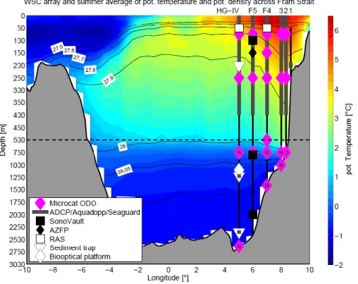
Spitsbergen Current (WSC) in Fram Strait (at the inflow of warm Atlantic water to the Arctic Ocean) as well as to other moorings in Fram Strait. The cross-section of the WSC array is shown in Figure 3. In total, 51 oxygen time series were obtained in 2016 to 2018 in Fram Strait between 20 m below the surface and 2650 m below the surface. The location of oxygen measurements for 2016-2018 is shown in Figure 2b.

Currently, a subset of the WSC array has oxygen sensors, and it is planned that this will be maintained in the future.

(10)

Figure 3. Cross-section across the deep Fram Strait along 79°N. The colour shows the average summer potential temperature.

The mooring and instrument locations of the volume transport monitoring array in the West Spitsbergen Current are shown.

Unlike many other records, some of the AWI records are from depths significantly below 1000 m. We assume that a previously undescribed pressure dependent problem exists in those situations (see also Section 3.4). In those records, there appears to be non-linear drift of the measured oxygen to lower values.

Seabird specifies that their optodes drift low by up to 2% per year. However, what was seen in the AWI records appears to be more than that.

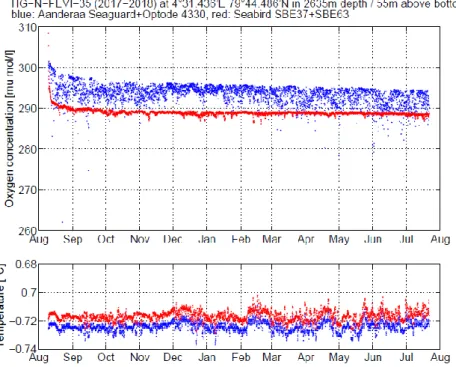
In 2635 m depth (55 m above the bottom), two instruments were deployed within 1 m of each other for a period of 11 months: Aanderaa Seaguard+Optode 4330 and SBE37+SBE63. As can be seen in Figure 4, both sensors drift non-linearly at the beginning of the record. The SBE37 starts at 308 μmol/l (note that this is after the sensor has reached its target depth on the mooring; the time before was already removed from the data set). Within a week, it settles to 290 μmol/l. This corresponds to a change of 6%, i.e. more than the stated 2% drift. Of course, a consideration is whether the recorded values correspond to a real change of the oxygen concentration in the water that was measured by the sensor. This appears unlikely for two reasons: The associated temperature records show real, but weak variability around temperatures of -0.72

°C. From previous work, it is known that the water in this region/depth warms by 0.005-0.01°C per year and that the temperature should reach -0.71°C in 2020 (von Appen et al., 2015). The temperature records agree with that expectation. The second reason is that a similar initial drift behavior is seen in multiple

instruments of the two kinds that were deployed for differing durations (1 vs. 2 years). If it was a real seasonal signal, then a similar drift from high to low should also occur in the middle of a two year deployment, but this kind of behavior was not observed.

(11)

Figure 4. Oxygen concentration and temperature measurements from an Aanderaa Seaguard+Optode 4330 (blue) and a Seabird SBE37+SBE63 (red) deployed in 2635 m from 2017 to 2018.

The other thing to note from Figure 4 is that the Aanderaa optode also has an initial drift, but its magnitude is smaller, from 302 μmol/l to 297 μmol/l (1.6 % in the first month). Unlike the Seabird optode, the

Aanderaa optode however appears to have a slow continuous drift to 295 μmol/l for the remainder of the one year deployment. Additionally, the Aanderaa measurement is much more noisy. It typically varies by more than 10 μmol/l within a month while the Seabird varies within roughly 2 μmol/l instead. It appears that there is no scatter above the maximum recorded oxygen value, while lower measurements occur quite often, making the distribution non-normal.

Winkler adjusted CTD rosette measurements during the deployment cruise (August 2017) and the recovery cruise (July 2018) showed oxygen concentrations of 306 and 302 μmol/l respectively. This suggests that initial Seabird measurements were a bit too high, while after the drift they were significantly too low.

Likewise, the initial Aanderaa measurements were a bit too high, while after the drift they were too low, but less far from the likely oceanic values than the Seabird sensor.

This highlights that a pre-deployment calibration of the moored instruments on the CTD rosette will not be helpful as the drift during the CTD cast (at the maximum a few hours duration) will be negligible compared to the drift during the entire deployment period. Likewise, post-deployment and pre-recovery CTD casts will be non-straightforward to use given that the drift to correct is not linear (with two CTD casts only two parameters---constant offset plus linear drift---could be determined). Considering typical cruise tracks additional time points to visit the deployed sensor are highly unlikely. This especially applies to a visit one month after deployment when the majority of the initial drift appears to have stopped.

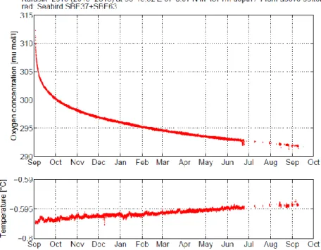
A few SBE37 instruments were also deployed at much greater depths, such as a record from 2015-2016 at 4571 m below the surface/140 m above the bottom (Figure 5). The slow increase in temperature again agrees with expectations of the warming of the deep Arctic Ocean and demonstrates the very weak

(12)

variability in water masses at the measurement location. In contrast, the oxygen record never settles. After a steep initial drift, the drift becomes less strong but remains at more than 5 μmol/l per year even after the first 6 months in the water. Over the duration of the deployment the drift exceeds 20 μmol/l (6%). Towards the end of the deployment, the sensor appears to have some battery issues which results in only

intermittent data return in July-September 2016. However, the drift per unit time (rather than drift per number of measurements) seems to stay the same. This would suggest an effect independent of the number of measurements (e.g. optical burning or similar effects).

Figure 5. Oxygen concentration and temperature measurements from a Seabird SBE37+SBE63 deployed in 4571 m from 2015 to 2017.

(13)

Figure 6. Temperature, oxygen concentration, and oxygen saturation measurements from two Seabird SBE37+SBE63 deployed in 25/28 m from 2016 to 2018.

Other oxygen sensors were deployed as shallow as in the euphotic zone, which in partially sea-ice covered areas is a challenge given that top buoys are not possible. At a central location in the WSC array (Figure 6), separate instrument records exist from 25 m in 2016-2017 and from 28 m in 2017-2018. The known seasonal cycle in temperature (von Appen et al., 2016) is reproduced with cooling from 8°C in early September to 3°C in late April. Corresponding to this cooling, the oxygen concentrations slowly rise by 30 μmol/l. In winter the absolute values of the records indicate an undersaturation of roughly 95% or 92%. The different values in the two years likely are due to the different instruments. The fact that the mixed layer is not at 100% saturation in the cooling period is expected given that gas exchange rates are not large for small differences between atmospheric values and an undersaturated mixed layer. The cooling also constantly increases the oxygen concentration of 100% saturation requiring an oxygen flux into the mixed layer. Additionally, during the cooling period, the mixed layer deepens and entrains lower oxygen

concentration water from below. What the resulting expected mixed layer saturation should be can be calculated, but this has not been done. Therefore, it is not possible at this point to decide whether the 5%/8% undersaturation is real or is also related to instrument drift as described above for the instruments subjected to extreme pressures.

When the productive season starts, phytoplankton releases oxygen during photosynthesis. Using additional sensors on the mooring, the rapid oxygen concentration/saturation increase at the beginning of May 2018, was linked to the onset of stratification and increases in chlorophyll concentration as well as a decrease in light penetrating to 28 m. A complete sensor suite allows to establish this link to oxygen where available and the relatively inexpensive oxygen measurements then allow conclusions about other times (e.g. spring 2017) or locations where such sensor suites do not exist.

(14)

In conclusion, the expertise in how to handle and work with oxygen measurements is still under

development. But important lessons have been learnt that are being used to decide upon data handling including when to apply manufacturer calibrations, on-CTD rosette calibrations, as well as post-deployment and pre-recovery CTD casts.

2.2 Greenland-Scotland Ridge

2.2.1 Denmark Strait

The Denmark Strait Overflow is usually monitored with two moorings at the Denmark Strait sill (Figure 7 and Figure 8; Jochumsen et al., 2017). One mooring (DS1) is located at the deepest point of the passage (approx. 660 m) and is maintained by the Marine and Freshwater Research Institute Reykjavik, Iceland. A second mooring (DS2) is located approx. 10 km west of DS1 at a depth of about 580 m and is maintained by the Institute of Oceanography in Hamburg, Germany. The moorings are usually recovered and redeployed once a year (see e.g. Jochumsen et al., 2017 for further details).

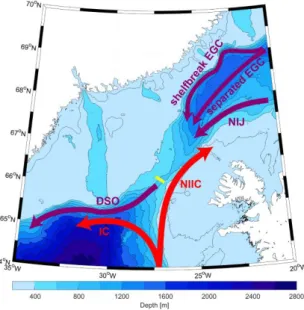
Figure 7. Map of the Denmark Strait and the location of the mooring array at the sill (yellow line). The schematic circulation indicates the pathway of the Denmark Strait Overflow (DSO) and its upstream sources: the branches of the East Greenland Current (EGC) and the North Icelandic Jet (purple). The warm and saline North Icelandic Irminger Current (NIIC, red) is the northward flowing current through the Denmark Strait, and the Irminger Current (IC) follows the Greenland shelf break southwestward.

(15)

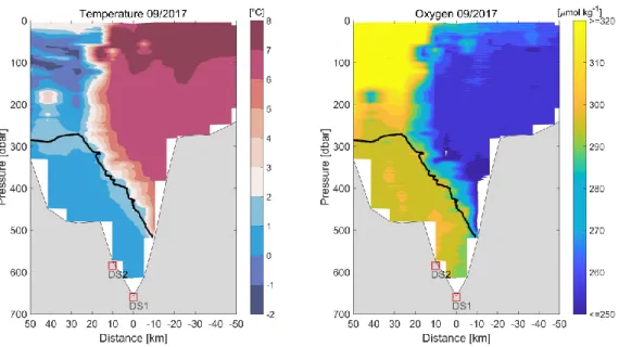
Figure 8. Sections of temperature (left) and oxygen (right) obtained during the Pelagia cruise 64PE426 in September 2017. The positions of the moorings DS1 and DS2 are indicated by the red squares. The thick black line shows the 27.8 kg m^-3isopycnal that is traditionally used to identify the DSO water.

The mooring design typically consists of an upward looking ADCP and a Seabird SBE 37 (MicroCAT), sitting approx. 5 m above the seabed (Figure 9). With funding from the AtlantOS and NACLIM projects, two SBE- SMP-ODO MicroCATs with SBE 63 oxygen sensors were purchased and installed on these two moorings.

Figure 9. Deployment and design of a mooring at the Denmark Strait Sill array. A MicroCAT (SBE37) with a SBE 63 oxygen sensor is installed at a depth of approx. 5 m above the sea bed.

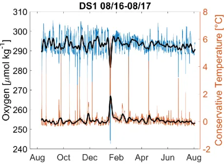
The oxygen sensor at DS1 was deployed in August 2016, recovered and redeployed in August 2017.

Unfortunately, the recovery attempt in 2018 failed and the instrument is considered lost. The one year-long time series of the hourly sampled oxygen and temperature are shown in Figure 10. The mean ± standard deviation of the oxygen content is 293 ± 6 μmol kg^-1.

(16)

Figure 10. Time series (August 2016 to August 2017) of oxygen (blue) and temperature (red) records at DS1. Thick black lines are 10-day low-pass filtered values.

The oxygen sensor at DS2 was deployed in September 2017, recovered and redeployed in August 2018, and is scheduled to be recovered in 2019. Calibration casts for mooring DS2 during deployment and recovery were done by attaching the MicroCATs to the CTD Rosette with 5 minute bottle stops during the upcast of the CTD profiles. The one year-long time series of the uncalibrated half-hourly sampled oxygen and temperature records are shown in Figure 11. The mean ± standard deviation of the (uncalibrated) oxygen content is 288 ± 4 μmol kg^-1. When final processing and calibration is completed the dataset will be made available and metadata uploaded to the OceanSITES database.

(17)

Figure 11. Time series (September 2017 to August 2018) of oxygen (blue) and temperature (red) records at DS2. Thick black lines are 10-day low-pass filtered values.

In addition to the above-mentioned important aspects of oxygen measurements in a global context, the new observations in the Denmark Strait may give further insight in to the sources and the variability of the Denmark Strait Overflow.

The Institute of Oceanography (Hamburg, Germany) received funding from the RACE project for the cruises during which DS2 was deployed and recovered.

2.2.2 Faroe Bank Channel

The Faroe Bank Channel (FBC) overflow has been monitored since 1995 using RDI Broadband ADCPs. In the beginning one mooring (NWFB) was deployed at the sill in the centre of the channel, but later an additional mooring (NWFC) was added, and in recent years these have both been continuously operational only interrupted by a few weeks for annual servicing of the instruments. Figure 12 shows a map of the FBC and a typical temperature section across the channel. The NWFB mooring is always embedded in overflow water, while the interface occasionally can pinch towards mooring NWFC. More details about the FBC overflow can be found in Hansen et al. (2016).

(18)

Figure 12. (a) Map of the topography of the Fare Bank Channel (FBC) area. Red dots indicate the location of the two ADCP moorings, while the red line shows the standard CTD section across the channel. A few stations are indicated with stars. (b) Temperature section based on data from stations indicated with stars in a). The data are from R/V Magnus Heinason cruise 1624 in June 2016. The two red dots indicate the approximate location (downstream) of the NWFB (right) and NWFC (left) moorings.

Overflow water typically fills the lower 200-300 m of the water column with Atlantic water overlying this. The temperature section in (b) was plotted using the Ocean Data View software (Schlitzer, R., Ocean Data View, https://odv.awi.de, 2018).

In 2001, a SBE-37SM MicroCAT was added to mooring NWFB in order to improve the temperature

measurements at the site, and both moorings are now usually equipped with a high precision temperature recorder (SBE-37, SBE-39 or similar). In 2015, a SBE-37SMP-ODO MicroCAT was funded by the AtlantOS and NACLIM projects to observe oxygen levels of the overflow water. This instrument was installed on the NWFB mooring and deployed for the first time in June 2016 and recovered in May 2017. The quality of the recorded data was good and thus the instrument was redeployed in June 2017 and recovered in May 2018.

Again the data were good and the instrument was redeployed in June 2018 with planned recovery in May 2019. Figure 13 shows the oxygen and temperature observations from the two completed deployments to date.

(19)

Figure 13. Oxygen (blue) and temperature (red) observations at site NWFB. Upper panel is from the deployment in June 2016;

lower panel is from the deployment in June 2017. Note the different scales in the panels. The oxygen data have not been corrected for the hysteresis effect (see Section 3.4) in the beginning of the deployments, but instrument performance has been compared to CTD observations (see text for details).

During the first deployment, a CTD cast was performed in April 2017 at the NWFB site, and a post-recovery calibration was done by attaching the MicroCAT to the CTD rosette; bottle stops lasted a few minutes at two different depth levels on the upcast. The CTD used for these comparisons was a SeaBird SBE9+ with an SBE43 dissolved oxygen sensor. The comparison between the deployed MicroCAT data and data from the CTD station at NWFB showed near identical (within instrument accuracy) temperature, salinity and oxygen readings – for oxygen the difference was approx. 6 µmol kg^-1. For the post-recovery calibration, this was also the case, but the difference between the MicroCAT and CTD oxygen readings at the deeper depth level (720 m) was larger (8.5 µmol kg^-1) than at the shallower depth level (171 m – 5.6 µmol kg^-1). The MicroCAT deployment data have also been compared with concurrent CTD observations at the upstream CTD section, but here some of the comparisons showed much larger differences (beyond the instrument accuracies).

These initial results thus indicate that CTD casts at the site during deployment and/or pre/post-deployment calibration casts can be used to verify or calibrate the MicroCAT readings.

2.3 OSNAP

2.3.1 Labrador Sea

CERC.Ocean (https://www.dal.ca/diff/cerc.html) at Dalhousie University in collaboration with GEOMAR deployed nine Aanderaa 4330 oxygen optodes on the 53N array of deep moorings in the Labrador Sea in May 2016 (Figure 14). The mooring array is a part of the OSNAP-WEST line, which is serviced every second year. These sensors were deployed as part of the VITALS project, with the primary goal to quantify

transport of oxygen in the Labrador Sea Water (LSW) out of the Labrador Sea. The oxygen sensors,

equipped with the single channel loggers (RBR), were deployed at strategic locations and were paired with the existing MicroCATs on the mooring array.

(20)

Figure 14. Schematic of the 53N mooring array (OSNAP-WEST) is shown on the left with the location of deployed optodes (red circles). Optode and its depiction on the mooring line during the deployment are shown on the right.

During the service cruise in 2018, data from these sensors were downloaded; the sensors were checked for drift and redeployed for another 2 years.

Upon deployment and recovery of the moorings in 2016 and 2018, a number CTD-DO casts were made for in situ sensor calibrations. In addition, CTD casts were conducted near the OSNAP moorings in conjunction with recovery and deployment of the moorings.

(21)

Figure 15. Time series of oxygen concentration and temperature for the sensors deployed on the K7 and K9 moorings in the Boundary Current in 2016-2018. Please note that the values are not corrected for in situ drift.

An example of uncalibrated data from K7 and K9 moorings is shown in Figure 15. As expected, deeper (1875 m and 2885 m) oxygen and temperature values show less variability, representing older NADW and DSOW. The shallower optodes show a clear convection signal manifesting itself in increased oxygen concentrations and colder temperatures during winter months (March 2018). It is worth noting that increase of oxygen at 1100 m depth is desynchronized from the oxygen increase at 600 m on K7 mooring, and happens with a ca. 1-1.5 month delay. A question stands whether convection occurs in the boundary current itself or convected waters are being partially mixed-in from the Labrador Sea interior.

Careful calibration of the optodes is necessary to access variability of oxygen content. Conditioning of optodes causes a non-linear drift during the first days-weeks of the deployment and should be taken into account when performing the final data calibration. In addition to pressure-related drift mentioned in Section 3.4, oxygen dissolved in the plastic materials of the sensors’ body or brackets may cause the observed non-linear drift: upon deployment oxygen leaks out and contaminates surrounding water. Thus plastic materials should be avoided where possible. Another recommendation is to keep the sensors wet at all times: drying out the foils may take 12-24h to adjust to water measurements. All these aspects should be taken into account and carefully addressed when assessing the observed drift of either instrumental or environmental origin.

(22)

Finally, calibrated data supported by the velocity and other data from the 53N mooring array will aid in quantifying transport of oxygen out of the Labrador Sea by the Labrador Current.

2.3.2 Rockall Trough

SAMS deployed three SeaBird SMP37-ODO’s and one Deep SeapHOx (combined SMP37-ODO and pH sensor) in the eastern Rockall Trough in May 2017. These sensors were deployed as part of the AtlantOS and ATLAS projects, with the overall aim of calculating nutrient and carbon fluxes through the basin.

Multiple linear regression equations, derived from hydrographic sections, will be used to reconstruct time- varying nutrient and carbon fields from mooring data which will then be multiplied by volume transports.

As method trials have shown that oxygen is required to ensure small residuals, particularly at mid-depths, the moored oxygen time series are a crucial part of these calculations.

The Deep SeaphOx was deployed at 50 m, with the SMP37-ODO’s at 750 m, 1000 m and 1600 m.

Instruments were successfully recovered in July 2018. On advice from the RAPID-ABC project, nearby CTD casts were conducted after deployment and prior to recovery in addition to the usual calibration dips.

Initial uncalibrated data are shown in Figure 16. Dissolved oxygen concentrations show the expected distribution with higher concentrations at the surface and 1600 m, and lower values in the mid water column. The record at 1600 m has the lowest variability, with the instrument at 750 m (rather than the 50 m sensor) showing the greatest variability. This probably reflects the 750 m sensors position in an area of rapidly changing oxygen concentrations between the oxygen-rich upper waters, and layer of reduced oxygen centred upon 1000 m. Another notable feature is the reduced variability at 50 m in the winter months compared to the summer. This is commonly seen in moored records and reflects the more homogenous nature of the water column in winter due to convection and mixing. When the effect of temperature is removed, and oxygen saturations are considered (Figure 16b), the pattern of variability remains with the record at 750 m showing the greatest variability. However, whilst saturation is close to 100 % at 50 m, saturations at 1600 m and 750 m are comparable at around 85 %. Both the lowest concentrations and saturations are seen at 1000 m which is unsurprising as this sensor was deliberately deployed to monitor the core of the lower oxygen layer.

(23)

Figure 16. Low-pass filtered time series of (a) oxygen concentrations (µmol kg^-1) and (b) oxygen saturations from the four moored oxygen sensors deployed in the eastern Rockall Trough. Please note that values are uncalibrated and have been filtered using a 48 hour Butterworth filter.

(24)

Figure 17. Time series of oxygen concentration (µmol kg^-1) for the sensor deployed at 1600 m in the eastern Rockall Trough showing the pressure-drift. Please note values are uncalibrated.

2.4 ABC Fluxes (RAPID-MOCHA-WBTS)

The Atlantic BiogeoChemical (ABC) Fluxes project (http://www.rapid.ac.uk/abc) began adding oxygen sensors to the RAPID mooring array in the subtropical North Atlantic in October 2015.

Table 1. Summary of the moored sensors and samplers deployed and recovered by the ABC fluxes project.

Deployment number

Deployment Recovery oxygen sensors pCO2 and pH sensor pairs

RAS Samplers

Cruise/Date Deployed (records recovered) ABC-0,

completed

JC103/

May 2014

DY039/

Nov 2015

12 (12)

6 (6): WB1/WBH2 6 (6): WB4

ABC-1

completed

DY039/

Nov 2015

JC145/

Apr 2017

24 (21)

6 (5): WB1/WBH2 6: WB4

6 (5): MAR1 6 (5): EB1

3 pairs of 1pCO2 and 1pH

1 (1pco2): WB4@50m 1 (0): MAR1@50m 1 (1pH): EB1@50m

4 (0)

WBH2@1500m WB4@50m MAR1@50m EB1@50m

(25)

ABC-2

In water

JC145/

Apr 2017

JC174/

Oct 2018

24

6: WB1/WBH2 6: WB4 6: MAR1 6: EB1

3 pairs

WB4@50m MAR1@50m EB1@50m ABC-3

planned

JC174/

Oct 2018

TBA/

Spring 2010 40

9: WB1/WBH2 9: WB4 9: MAR1 9: EB1 3: EBH3 1: EBH4

3 pairs:

WB4@50m MAR1@50m EB1@50m

The oxygen sensors were largely very reliable and the only data losses related to lost instruments (50 m, MAR1, ABC-1) and sensors that were collocated and reliant (for logging) on faulty pH sensors (50 m, MAR1 and EB1, ABC-1).

In the next sections we describe the data collected and their calibration. Ultimately these new data will inform the multiple linear regression used in the time series calculations.

Oxygen sensors and their calibration

The oxygen sensor chosen was a SeaBird ‘optical dissolved oxygen’ model SBE-63. We refer to these as

‘ODO’ sensors. This sensor is deployed attached to a SBE MicroCAT, which provides temperature and salinity data and acts as the data logger. In order to ensure that the core RAPID measurements would not be compromised, an extra MicroCAT was procured by ABC to carry each ODO, so that the ABC

measurements were ‘stand-alone’. In most instances, the ABC MicroCAT/ODO was deployed alongside a core RAPID MicroCAT.

Pre-ABC funding from NOC provided 12 instruments for an early trial deployment. ABC provided 36 new instruments to provide a stock of 48, so that 24 could be used on each ABC deployment without the need to recover and re-deploy instruments on the same cruise and allow for calibration between deployments.

The pre-ABC trial (‘ABC-0’, Table 1) deployed 12 sensors at the 6 nominal depths on the two WB locations, as summarised in table 1. All instruments provided full records.

Deployment ABC-1: 24 new instruments were deployed at 4 locations. WB1/WBH2 and WB4 as in ABC-0, plus MAR1 and EB1. In ABC-1, three of the shallow instruments had the further addition of pH sensors (WB1, MAR1, and EB1). The combined MicroCAT/ODO/pH instrument is referred to as a SeapHOx. None of the SeapHOx instruments returned a full record: one exhausted its batteries early, one leaked (resulting in the loss not just of the pH data but also the oxygen data), and the top of the MAR1 mooring was lost to trawling. However, the 21 stand-alone MicroCAT/ODO instruments all returned full records.

(26)

Deployment ABC-2: 12 new instruments and 12 from ABC-0 were deployed to replace the ABC-1 array.

These instruments will be recovered in October 2018.

Deployment ABC-3: The array will be recovered and redeployed in October 2018. This will include all the instruments recovered from ABC-1 (with lost instruments replaced). In addition, 16 instruments anticipated to be recovered from ABC-2 will be immediately re-deployed to enhance the array. This will provide time series at extra depths at the four established sites: 250 m, 600 m and 1000 m. It will also extend the array closer to the eastern boundary at EBH3 (50 m, 400 m, and 750 m) and EBH1 (750 m). After studying the data from ABC-0 and ABC-1, the 800 m instruments at WB1 and WBH2 will be moved to 750 m. The choice of 16 instruments for immediate redeployment reflects that there is insufficient time to prepare the final 5 ODOs recovered for immediate redeployment, and allows the SeapHOxs from ABC-2 to be returned to NOC or SBE for evaluation of the pH sensors.

Measurements

Data available for analysis at the time of writing (Jun 2018) are the 12 records from ABC-0, and the 21 records from ABC-1. There is substantial variability in the oxygen ‘signal’ at each instrument caused by the vertical migration of isotherms relative to the instruments. This occurs either as internal waves pass the moorings and the ocean moves, or as the instruments move in the vertical when fluctuating currents cause the mooring to lean over and the instruments are displaced deeper. This effect has been removed by making use of shipboard temperature-oxygen profiles obtained on the deployment cruises. Each oxygen record can be adjusted to oxygen at a nominal temperature, by adding the oxygen fluctuation

corresponding to the temperature fluctuation, defined by the shipboard profile. The residual after this adjustment is the part of the oxygen signal not correlated with temperature. At the eastern boundary 800 m instrument, a further part of the residual can be accounted for by correlation with salinity variations.

The conventional approach to calibration of MicroCAT salinity is to attach the instruments to a ship-borne CTD package and perform a vertical cast with pauses at 12 depths to obtain a good MicroCAT/shipCTD comparison. These comparisons are used to determine an adjustment for each MicroCAT so that the data are consistent with an absolute reference. This approach was used for the ODO sensors as well. However, we have found that the behaviour of the ODOs when deployed on a mooring is different than when deployed on a ship-borne CTD package. In particular, the ODOs drift towards lower oxygen values over the 18 months mooring deployment. The characteristics of this creep seem to be reasonably consistent between instruments: The magnitude is pressure dependent. For the instruments at 3500 m, the creep is between 9 and 15 μmol kg^-1 over each 18-month deployment. This is 3.5% of the oxygen concentration, and an order of magnitude larger than the ocean variability at that depth. This creep can be modelled with an exponential decay with multiple timescales. Typically, there is a fast creep with a timescale of 3 to 5 days, and a slower creep with a timescale of 150 to 200 days. The slow creep has not normally reached a stable value within the 500 days of each deployment.

The creep due to pressure seems to be reversible as soon a sensor is returned to surface pressure.

Therefore, a post-deployment ‘calibration’ does not enable us to quantify and remove the effect. The most useful data for evaluating the moored oxygen data are ship-based measurements made near to the moorings.

(27)

We conclude that the small creep in deep instruments means that for the time being this technology is unable to distinguish small trends in deep ocean oxygen from instrumental artefacts. Monitoring oxygen in the deep ocean therefore requires ship-based measurements, or possibly the use of Deep Argo floats with oxygen sensors. The pressure effect resets when the sensor is returned to surface pressure, so Deep floats that regularly return to the surface may offer a better option.

The manufacturer, SBE, has offered an explanation for the creep in terms of the slow compression of the material that carries the oxygen-sensitive part of the ODO.As seen in other sections of this report, other groups have encountered comparable problems with their long-term deployments of this instrument at depths deeper than 1500 m, and a community wide analysis may aid to characterise this behaviour. We will review the pressure-sensitive behaviour of the sensors after the recovery of ABC-2, and then reach a conclusion about the way to calibrate and adjust the sensor data.

Enhancement of upper ocean array for ABC-3

Analysis of the data so far suggests that at the three deeper levels in the array (1500 m, 2000 m, and 3500 m), the residual oxygen signal not correlated with temperature is too small to be reliably measured with ODO sensors. The residual is small and cannot be reliably extracted from the creeping ODO data. The possible exception to this may be EB1, where the deep signal is larger, but we need to see data from ABC-2 before we can make a judgement.

In order to maximise the data return from the three ABC deployments, many of the ABC-2 instruments will be redeployed in ABC-3, enhancing the upper ocean measurements at WB1, WB4, MAR1 and EB1, and adding instruments further inshore at EBH3 and EBH4. The primary ABC-3 measurements will be from fresh instruments prepared ashore, and the additional measurements will be from the redeployed instruments.

We have maintained the deployment of a full set of deep (> 1500 m) instruments into ABC-3, even though we are doubtful that they will return measurements containing a significant signal. We cannot justify removing them from the array after just ABC-1, and the decision to maintain them in ABC-3 needs to be taken before the recovery of ABC-2. We anticipate that when ABC-2 has been fully analysed, we will conclude that it is only useful to deploy moored oxygen sensors in the upper 1500 m or so of the array. The enhanced upper-ocean coverage in ABC-3 will help to define the useful density of upper ocean

measurements.

(28)

Figure 18. Moored oxygen data from WB4 during ABC-0 and ABC-1. The left panels show raw ODO data. The right panels are the residuals after adjustment for temperature variations. The deepest three levels are dominated by the sensor creep due to prolonged exposure to pressure. The biggest excursions at 400 and 800m are associated with temperature variations and are removed by the temperature adjustment. The panels, top to bottom are data from the six levels: 50m, 400m, 800m, 1500m, 2000m, and 3500m. Each panel contains data from two instruments: the ABC-0 and ABC-1 deployments are divided around day 320 corresponding to November 2015.

2.5 MOVE

The MOVE project started making oxygen measurements on two moorings in 2016. The moorings are at the western and eastern ends of the MOVE 16°N section, just east of Guadeloupe Island in the west and west of Researcher Ridge in the east. Each mooring has oxygen sensors at two depths, near 1800 and 3700 meters. The depths coincide with the depths of specific components of the North Atlantic Deep Water (NADW): the depths match the Labrador Sea Water and Denmark Strait Overflow Water cores (see Figure 3 in Send et al., 2011). Additional instruments on these moorings measure temperature and salinity

throughout the water column, and these have been in place since 2000. Calibration casts with ship-based CTDs and water samples are routinely done before deployments and after recoveries (Kanzow et al., 2006), both for the salinity and now also the oxygen instruments. At the time of writing, the MOVE oxygen data have not been processed, but they will become available through the OceanSITES database once processing is completed. MOVE scientists are interested in comparing oxygen data across multiple arrays, and will be happy to participate in collaborative analyses.

(29)

3 Best practice for Oxygen measurements at TMA sites 3.1 Principles of operation

Commercially available oxygen sensors for oceanographic applications use one of two operating principles to measure oxygen concentration:

1) electrochemical (polarographic membrane) sensors; such as the Sea-Bird Scientific SBE-43 2) optode-based sensors; such as the Sea-Bird Scientific SBE-63, the Aanderaa Data Instruments

3830/3835, 4330 and 4831 sensors, and the JFE Rinko sensors.

Coppola et al. (2013) provide an overview of these sensors and their main advantages & disadvantages, moreover an in-depth review of the optode sensing principle can be found in Bittig et al. (2018).

Electrochemical sensors are flow-dependent (as oxygen is consumed during the measurement and needs to be replenished) and can drift significantly; but have relatively fast response times. This makes

electrochemical membrane sensors the preferred technology for (ship-based) profiling applications, where fast response is needed and where calibration samples are readily available. Generally, optode sensors are more accurate and require less maintenance, but also require concurrent salinity measurements, in order to correct for the salinity effect of dissolved oxygen in sea water. Because they are relatively more stable, they have become the standard measuring technique for moored applications.

3.2 Calibration

In general, the adherence to the manufacturer’s guidance - in particular their recommended procedures for transport, storage, plumbing, routine care and factory maintenance/calibration - results in the collection of good quality oxygen observations. Because recommendations vary by manufacturer and sensor, these are not provided here.

CTD oxygen sensor calibration procedures for ship-based profile measurements have been established by the GO-SHIP community (Uchida et al., 2010). Bittig et al. (2018) published a thorough review of oxygen optode sensor calibration.

For optode sensors, the manufacturer will measure the optode response during factory calibration for a number of oxygen and temperature levels across an adequate range to determine a calibration matrix, also called a multi-point calibration (Bittig et al., 2018). It is recommended to have sensors calibrated both before and after deployment, to get a reasonable estimate of the calibration error, and therefore the measurement error. Indeed, the multi-point calibration method is a calibration over the whole parameter space in order to describe the general characteristics of the sensing foil (actually: this is the unique

combination of the sensing foil and instrument). In contrast, an in-situ calibration (during a ship cruise) is always a calibration against a subset of this parameter space. This method is used to correct for potential drifts of the sensing foil, but is not able to describe the general foil characteristics. Hahn et al. (2014) have conducted on-board calibrations for 37 Aanderaa optode oxygen sensors, deployed on several moorings in the eastern tropical Atlantic. By taking into account calibrations conducted directly before and after the deployment period (18 months on average), they identified an overall average root mean square error for these oxygen sensors of better than 3 μmol/kg.

(30)

3.3 Instrument drift

For electrochemical sensors, a predictable drift occurs due to a loss of sensitivity. As shown by Coppola et al. (2013; their Figure 4), this drift is noticeable over a period of 1-2 weeks. This highlights the unsuitability of electrochemical sensors on prolonged mooring deployments.

Oxygen optode sensors experience a significant amount of drift during storage (Bittig et al., 2018), losing sensitivity of the order of 5% per year. Sensor drift during deployment is much lower, and this drift can be corrected by calibrating the sensor immediately prior to deployment. Drift during deployment was found to be minimal: Tengberg et al. (2006) did not measure noticeable drift from Argo-float mounted sensors deployed in the Labrador Sea for 1.6 years.

3.4 Pressure effects on oxygen measurements

During deployments of oxygen sensors on TMA moorings at great depth a slow drift to lower oxygen concentrations has been detected. From comparison of time series at different depths and TMA sites, this issue seems to be most noticeable for sensors deployed at depths greater than 1,500 m. The drift can be seen in the sections presenting results from Fram Strait, Faroe Bank Channel, Denmark Strait, Labrador Sea, Rockall Trough, and RAPID. A thorough description of the issue has been highlighted in the Fram Strait and ABC Fluxes sections. At the workshop held in Edinburgh, several groups highlighted the issue, and a

community-wide effort is now underway to identify the source of the problem, as well as reach a consensus method for removing the drift from existing time series.

3.5 Recommended best practice

The following suggestions are considered the current best practice to obtain oxygen observations from moored optode sensors

● Send the instruments for factory calibration prior to deployment (optionally). Each oxygen sensor (i.e. each unique combination of a sensing foil and instrument) should be subject to at least one multi-point calibration during its lifetime in order to describe the general characteristics of this sensor (Bittig et al., 2018). It is worth noting that sensing foils may not be calibrated while mounted on their target instrument, and therefore it is cautious to assume such a multi-point calibration has not been performed by the manufacturer.

● Undertake pre- and post-deployment calibration casts using the ship’s CTD carousel, obtaining coincident water samples for Winkler titration analysis. Bottle stops on the upcast are

recommended to be 10 to 15 minutes long. For calibration of sensors at shallower depths, shorter bottle stops (of the order of 5 minutes) may be possible.

○ Trigger the closure of the carousel’s bottles close to the end of the bottle stop.

○ To help reduce the noise level, take all the Winkler samples and calibrate the CTD oxygen sensor and use the so calibrated CTD oxygen as “measurement”, in addition to the bottle stop discrete sample comparisons.

○ During analysis of the pre-/post-deployment CTD cast, examine drift during the bottle stop, and choose the values towards the end of the stop for calibration.

(31)

○ For instruments which will be deployed shallower than 1500 metres, don’t undertake the pre-deployment calibration cast to depths greater than 1500 m to avoid storing pressure effects in the sensor.

● Perform an additional on-board calibration in the laboratory at extreme oxygen concentrations (0%

saturation forces with Na2SO3 and 100% saturation using an aquarium pump). This expands the parameter space for calibration, and can be particularly important when deploying in low oxygen regions, which may be episodically measured during the mooring deployment, particularly at shallow depths. As the optode measurements (phase) are highly dependent on temperature, it is beneficial to change the temperature of the bath if possible (e.g. perform calibration in a freezer room +7°C)

● To calibrate sensors deployed in deeper waters (>1500 m) and to measure performance during the deployment, collect a CTD station close to the mooring site after deployment/before recovery.

Taking such a measurement right before recovery can be especially informative on sensor

performance on the mooring, before the pressure is changed during recovery. For deep (>1500 m) deployments, CTD profiles immediately after deployment and before recovery are critical, as the sensors won’t equilibrate to pressure effects during pre-/post-deployment calibration casts when stops are too short to account for the impacts on the time scales of days/weeks/months (as highlighted in section 3.4).

3.6 OceanSITES metadata provision

OceanSITES encourage principal investigators to work towards the FAIR data principles (Findable, Accessible, Interoperable, and Reusable) for their observations, and to make the observing efforts add value to the international context. Therefore, it is recommended to add information for each

site/deployment to the OceanSITES metadata database (further referred to as the OceanSITES database).

A “how-to” document on adding metadata to the OceanSITES database guides principal investigators through the process of uploading details for their mooring deployments to the OceanSITES database.

Individual assistance can also be obtained by emailing the OceanSITES technical coordinator (Long Jiang).

At this stage, only a few TMA sites have added their respective metadata to the global system, but as part of this report, principal investigators will endeavour to add the metadata for oxygen time series to the global system. The oxygen observational data time series (as seen in figures above) may not be provided currently as OceanSITES files but can be linked to the respective instrument at the JCOMMOPS website for the respective deployment.

(32)

4 Conclusions

Sustained observations of oxygen are critical to address some of the major societal challenges related to the impacts of climate change and ocean deoxygenation. Oxygen is fundamental to sustaining the ocean’s ecosystems and plays an important role in global biogeochemical cycles.

Oxygen sensor technology, sensor calibration techniques and data analysis are now well established within the oceanographic community, and reliable oxygen observations can now be collected with relative ease.

As part of the AtlantOS project, several Transport Mooring Arrays deployed oxygen sensors at established mooring sites (Section 2). Adding oxygen sensors to these Eulerian platforms is advantageous over sensors on Lagrangian profiling floats, as mooring sites are often in fast-moving boundary currents, where profiling floats sampling is scarce. Moreover, the concurrent transport and oxygen observations provide an

opportunity to study fluxes of nutrients and carbon at key locations. To further aid the successful inclusion of oxygen sensors on the TMA moorings, some best practice guidance has been presented in Section 3.5.

In addition, good metadata records and FAIR data principles will ensure these oxygen measurements add value to the global observing efforts.

Several groups have identified issues with a drift to lower measured concentrations for sensors deployed at depths greater than 1,500 m. This drift occurs on timescales of weeks to months. A community-wide effort is now underway to identify the source, and find a consensus approach to deal with this issue in existing datasets.

5 Acknowledgements

The contributors to this report would like to acknowledge the additional support received from the following projects:

 AtlantOS (EU's H2020 grant agreement No 633211), ATLAS (European Union’s Horizon 2020 research and innovation programme under grant agreement No 678760), NACLIM (EU's FP7 grant agreement No 308299), Blue-Action (EU's H2020 grant agreement No 727852). This output reflects only the authors’ views and the European Union cannot be held responsible for any use that may be made of the information contained therein.

 the United Kingdom’s Natural Environment Research Council programs UK-OSNAP, the Extended Ellett Line, and ACSIS (National Capability).

 Oxygen sensors on the RAPID array were funded by the UK's Natural Environment Research Council RAPID AMOC program through ABC fluxes (grant: NE/M005046/1).

 Support for this study was provided by the Helmholtz Infrastructure Initiative FRAM. Ship time was provided under grants AWI_PS94_00, AWI_PS99_00, AWI_PS100_01, AWI_PS101_01,

AWI_PS107_00, and AWI_PS114_01.

 Sonderforschungsbereich 754 „Climate-Biogeochemistry Interactions in the Tropical Ocean“

(founded by the Deutsche Forschungsgemeinschaft (DFG))

 ‘‘RACE II – Regional Atlantic Circulation and Global Change’’ funded by the German Federal Ministry for Education and Research (BMBF #03F0729B)

 MOVE was supported by NOAA's Ocean Observing and Monitoring Division (OOMD).

 VITALS

(33)

6 References

von Appen, W.-J., U. Schauer, T. Hattermann, A. Beszczynska-Möller. 2016. Seasonal Cycle of Mesoscale Instability of the West Spitsbergen Current. Journal of Physical Oceanography, 46: 1231–1254.

doi:10.1175/JPO-D-15-0184.1

von Appen, W.-J., U.Schauer, R. Somavilla, E. Bauerfeind, A. Beszczynska-Möller. 2015. Exchange of warming deep waters across Fram Strait. Deep-Sea Research Part I-Oceanographic Research Papers, 103:

86-100. doi:10.1016/j.dsr.2015.06.003

Bittig, H. C., A. Körtzinger, C. Neill, E. van Ooijen, J.N. Plant, J. Hahn et al. 2018. Oxygen Optode Sensors:

Principle, Characterization, Calibration, and Application in the Ocean. Frontiers in Marine Science, 4: 429.

doi:10.3389/fmars.2017.00429.

Bopp, L., C. Le Quéré, M. Heimann, A.C. Manning, P. Monfray. 2002. Climate‐induced oceanic oxygen fluxes:

Implications for the contemporary carbon budget. Global Biogeochemical Cycles, 16(2): 6-1.

doi:10.1029/2001GB001445.

Bourlès, B., P. Brandt, N. Lefevre, J. Hahn. 2018. PIRATA data system upgrade Report. Available online at https://www.atlantos-h2020.eu/download/deliverables/AtlantOS_deliverable_D3-9_v1.pdf (last accessed 29 March 2019)

Brandt, P., H. W. Bange, D. Banyte, M. Dengler, S.-H. Didwischus, T. Fischer et al. 2015. On the role of circulation and mixing in the ventilation of oxygen minimum zones with a focus on the eastern tropical North Atlantic, Biogeosciences, 12 (2): 489-512. doi:10.5194/bg-12-489-2015.

Breitburg, D., L. A. Levin, A. Oschlies, M. Grégoire, F. P. Chavez, D. J. Conley et al. 2018. Declining oxygen in the global ocean and coastal waters. Science, 359 (6371): eaam7240. doi:10.1126/science.aam7240 Clark Jr., L. C., R. Wolf, D. Granger, Z. Taylor. 1953. Continuous recording of blood oxygen tensions by polarography. Journal of Applied Physiology, 6 (3): 189-193. doi:10.1152/jappl.1953.6.3.189

Codispoti, L. A., J.A. Brandes, J.P. Christensen, A.H. Devol, S.W.A. Naqvi, H. W. Paerl, T. Yoshinari. 2001. The oceanic fixed nitrogen and nitrous oxide budgets: Moving targets as we enter the anthropocene? Scientia Marina, 65(S2): 85-105. doi:10.3989/scimar.2001.65s285.

Codispoti, L. A. (2010). Interesting Times for Marine N2O. Science, 327(5971), 1339 LP-1340.

https://doi.org/10.1126/science.1184945

Coppola, L., F. Salvetat, L. Delauney, D. Machoczek, J. Karstensen, V. Thierry et al. 2013. White paper on dissolved oxygen measurements: scientific needs and sensors accuracy. Jerico Project. Available online at http://www.jerico-ri.eu/download/filebase/White%20paper%20DO_final%20-copyright.pdf.

Gruber, N. & Co-Authors (2010). "Adding Oxygen to Argo: Developing a Global In Situ Observatory for Ocean Deoxygenation and Biogeochemistry" in Proceedings of OceanObs’09: Sustained Ocean

Observations and Information for Society (Vol. 2), Venice, Italy, 21-25 September 2009, Hall, J., Harrison, D.E. & Stammer, D., Eds., ESA Publication WPP-306, doi:10.5270/OceanObs09.cwp.39.

(34)

Gruber, N. (2011). Warming up, turning sour, losing breath: ocean biogeochemistry under global change.

Philosophical Transactions of the Royal Society A: Mathematical, Physical and Engineering Sciences, 369(1943), 1980–1996. https://doi.org/10.1098/rsta.2011.0003

Gruber, N., Clement, D., Carter, B. R., Feely, R. A., Heuven, S. Van, Hoppema, M., … Key, R. M. (2019). The oceanic sink for anthropogenic CO 2 from 1994 to 2007, 1199(March), 1193–1199.

Hahn, J., P. Brandt, R. J. Greatbatch, G. Krahmann, A. Kortzinger. 2014. Oxygen variance and meridional oxygen supply in the Tropical North East Atlantic oxygen minimum zone. Climate Dynamic, 43 (11): 2999- 3024, doi:10.1007/s00382-014-2065-0.

Hansen, B., K. M. Húsgarð Larsen, H. Hátún, S. Østerhus (2016). A stable Faroe Bank Channel overflow 1995–2015. Ocean Science, 12: 1205-1220. doi:10.5194/os-12-1205-2016.

Jochumsen, K., M. Moritz, N. Nunes, D. Quadfasel, K. M. Larsen, B. Hansen, H. Valdimarsson, S. Jonsson.

2017. Revised transport estimates of the Denmark Strait Overflow. Journal of Geophysical Research, 122:

3434–3450. doi:10.1002/2017JC012803.

Kanwisher, J. 1959. Polarographic Oxygen Electrode. Limnology and Oceanography, 4 (2): 210-217.

doi:10.4319/lo.1959.4.2.0210

Kanzow, T., U. Send, W. Zenk, A.D. Chave, M. Rhein. 2006. Monitoring the integrated deep meridional flow in the tropical North Atlantic: Long-term performance of a geostrophic array. Deep Sea Research Part I:

Oceanographic Research Papers, 53 (3): 528-546. doi:10.1016/j.dsr.2005.12.007.

Karstensen, J., L. Stramma, M. Visbeck. 2008. Oxygen minimum zones in the eastern tropical Atlantic and Pacific oceans. Progress in Oceanography, 77(4): 331-350. doi:10.1016/j.pocean.2007.05.009.

Kiel Declaration. 2018. The Ocean is losing its breath. Kiel Declaration on Ocean Deoxygenation by participants of the international conference “Ocean Deoxygenation: Drivers and Consequences – Past – Present – Future”, 3-7 September 2018, in Kiel, Germany. Available at https://www.ocean-

oxygen.org/declaration.

Körtzinger, A., J. Schimanski, U. Send. 2005. High quality oxygen measurements from profiling floats: A promising new technique. Journal of Atmospheric and Oceanic Technology, 22 (3): 302-308.

doi:10.1175/JTECH1701.1

Oschlies, A., P. Brandt, L. Stramma, S. Schmidtko. 2018. Drivers and mechanisms of ocean deoxygenation.

Nature Geoscience, 11 (July): 467–473. doi:10.1038/s41561-018-0152-2

Sabine, C. L., R. A. Feely,N. Gruber, R.M. Key, K. Lee, J. L. Bullister, et al. 2004. The Oceanic Sink for Anthropogenic CO2. Science, 305 (5682): 367–371. doi:10.1126/science.1097403.

Sarmiento, J., N. Gruber. 2006. Ocean Biogeochemical Dynamics. Princeton Univ. Press, Princeton, N. J.

Sarmiento, J. L., and J. C. Orr (Vol. 36).

Schmidtko, S., L. Stramma, M. Visbeck. 2017. Decline in global oceanic oxygen content during the past five decades. Nature, 542(7641): 335-339. doi:10.1038/nature21399.

(35)

Send, U., M. Lankhorst, T. Kanzow. 2011. Observation of decadal change in the Atlantic Meridional Overturning Circulation using 10 years of continuous transport data. Geophysical Research Letters, 38:

L24606. doi:10.1029/2011GL049801.

Talley, L. D., R. A. Feely, B. M. Sloyan, R. Wanninkhof, M. O. Baringer, J. L. Bullister, et al. 2016. Changes in ocean heat, carbon content, and ventilation: A review of the first decade of GO-SHIP global repeat

hydrography. Annual Review of Marine Science, 8: 185-215. doi:10.1146/annurev-marine-052915-100829.

Tengberg, A., J. Hovdenes, H. J. Andersson, O. Brocandel, R. Diaz, D. Hebert et al. 2006. Evaluation of a lifetime‐based optode to measure oxygen in aquatic systems. Limnology and Oceanography: Methods, 4(2):

7-17. doi:10.4319/lom.2006.4.7.

Uchida, H., T. Kawano, I. Kaneko, M. Fukasawa. 2008. In Situ Calibration of Optode-Based Oxygen Sensors.

Journal of Atmospheric and Oceanic Technology, 25 (12): 2271–2281. doi:10.1175/2008JTECHO549.1.

Uchida, H., G.C. Johnson, K.E. McTaggart. 2010. CTD Oxygen Sensor Calibration Procedures. In The GO-SHIP Repeat Hydrography Manual: A Collection of Expert Reports and Guidelines. Hood, E.M., C.L. Sabine, and B.M. Sloyan, eds. IOCCP Report Number 14, ICPO Publication Series Number 134. Available online at:

http://www.go-ship.org/HydroMan.html.

Winkler, L. W. 1888. Die bestimmung des im wasser gelösten sauerstoffes. Berichte der deutschen chemischen Gesellschaft, 21 (2): 2843-2854. doi:10.1002/cber.188802102122