Interannual variability of the Atlantic North Equatorial
1
Undercurrent and its impact on oxygen
2
K. Burmeister1, J. F. L¨ubbecke1,2, P. Brandt1,2, and O. Duteil1
3
1GEOMAR Helmholtz Centre for Ocean Research Kiel, D¨usternbrooker Weg 20, 24105 Kiel, Germany
4
2Christian-Albrechts-Universit¨at zu Kiel, Christian-Albrechts-Platz 4, 24118 Kiel, Germany
5
Key Points:
6
• Interannual variability of North Equatorial Undercurrent in an ocean general cir-
7
culation model is linked to Atlantic Meridional Mode
8
• Oxygen supply by the North Equatorial Undercurrent towards the Eastern Trop-
9
ical North Atlantic depends on the pathway of its source waters
10
• Different supply routes might explain discrepancies between simulated and observed
11
oxygen supply by the North Equatorial Undercurrent
12
Corresponding author: Kristin Burmeister,kburmeister@geomar.de
This article has been accepted for publication and undergone full peer review but has not been through the copyediting, typesetting, pagination and proofreading process which may lead to differences between this version and the Version of Record. Please cite this article as doi:
10.1029/2018JC014760
Abstract
13
The North Equatorial Undercurrent (NEUC) has been suggested to act as an important
14
oxygen supply route towards the oxygen minimum zone in the Eastern Tropical North
15
Atlantic. Observational estimates of the mean NEUC strength are uncertain due to the
16
presence of elevated mesoscale activities, and models have difficulties in simulating a realistic
17
NEUC. Here we investigate the interannual variability of the NEUC and its impact onto
18
oxygen based on the output of a high-resolution ocean general circulation model (OGCM)
19
and contrast the results with an unique data set of 21 ship sections along 23◦W and a
20
conceptual model. We find that the interannual variability of the NEUC in the OGCM is
21
related to the Atlantic Meridional Mode (AMM) with a stronger and more northward NEUC
22
during negative AMM phases. Discrepancies between OGCM and observations suggest a
23
different role of the NEUC in setting the regional oxygen distribution. In the model a
24
stronger NEUC is associated with a weaker oxygen supply towards the east. We attribute
25
this to a too strong recirculation between the NEUC and the northern branch of the South
26
Equatorial Current (nSEC) in the OGCM. Idealized experiments with the conceptual model
27
support the idea that the impact of NEUC variability on oxygen depends on the source
28
water pathway. A strengthening of the NEUC supplied out of the western boundary acts
29
to increase oxygen levels within the NEUC. A strengthening of the recirculations between
30
NEUC and the nSEC results in a reduction of oxygen levels within the NEUC.
31
Plain Language Summary
32
In the eastern tropical North Atlantic a zone of low-oxygen waters exists between
33
100m and 700m due to high oxygen consumption and a weak exchange of water masses.
34
Long-term oxygen changes in this zone have been reported with potential impacts on,
35
e.g., ecosystems including fish populations. The water masses in that region are exchanged
36
among others via weak eastward and westward currents. The mean eastward flowing North
37
Equatorial Undercurrent (NEUC) transports oxygen-rich waters from the western basin
38
into the eastern low-oxygen zone suggesting that a stronger NEUC supplies more oxygen-
39
rich water towards the eastern basin.
40
In this study we investigate the year-to-year variability of the NEUC and its im-
41
pact on oxygen. For our analysis, we are using ship observations and model simulations.
42
We find some discrepancies between them that we attribute to a too strong recircula-
43
tion between the NEUC and the westward flowing current just south of it in the model.
44
This recirculation impacts the variability of the eastward oxygen supply as the westward
45
current is transporting low-oxygen waters. In the model, a higher recirculation between
46
the currents results in a stronger NEUC transporting lower-oxygen waters, a mechanism
47
for oxygen variability that could not be conjectured from observations so far.
48
1 Introduction
49
The oxygen concentration in the oceans is controlled by the interaction of physical and
50
biogeochemical processes. Oxygen is supplied to the ocean by photosynthesis or air-sea
51
gas exchange and it is transported into the ocean interior by advection and mixing (e.g.
52
Brandt et al., 2015; Karstensen et al., 2008; Stramma et al., 2008). Oxygen is consumed
53
by respiration, e.g. by remineralization of sinking particles (Matear & Hirst, 2003). Locally
54
advection and mixing can also act to decrease oxygen levels, depending on the background
55
oxygen field (Brandt et al., 2010; Hahn et al., 2014).
56
The tropical Atlantic is characterized by a complex system of zonal currents that can
57
transport oxygen-rich waters from the western boundary eastwards towards the Eastern
58
Tropical North Atlantic (ETNA) Oxygen Minimum Zone (OMZ) or oxygen-poor waters
59
westward (Fig. 1). Consequently, the zonal advection of oxygen-rich water masses from the
60
western boundary by eastward flowing ocean currents has been identified as an important
61
ventilation process for the ETNA OMZ, especially in the upper 130 to 300 m (Brandt et al.,
62
2015; Hahn et al., 2014, 2017). The most important currents are the main wind-driven ones
63
such as the Equatorial Undercurrent (EUC), the North Equatorial Undercurrent (NEUC)
64
and the northern branch of the North Equatorial Countercurrent (nNECC) (e.g. Bourl`es
65
et al., 2002; Pe˜na-Izquierdo et al., 2015; Schott et al., 2004). Below the wind-driven ocean
66
circulation, the flow field in the ETNA OMZ is characterized by eddy-driven, weak latitudi-
67
nal alternating zonal jets (Ascani et al., 2010; Brandt et al., 2010; Maximenko et al., 2005;
68
Ollitrault & Colin de Verdi`ere, 2014; Qiu et al., 2013).
69
Oxygen levels in the ETNA OMZ are declining in accordance with global deoxygenation
70
(Schmidtko et al., 2017; Stramma et al., 2008). Superimposed on this multidecadal trend
71
are interannual to decadal variations. The identification of the mechanisms of long-term
72
oxygen changes is challenging because of large uncertainties in the observed oxygen budget
73
terms (Hahn et al., 2017; Oschlies et al., 2018). Furthermore, large biases in the oxygen
74
distribution in ocean models hamper the analysis of OMZ variability (e.g. Cabr´e et al., 2015;
75
Dietze & Loeptien, 2013; Duteil et al., 2014; Oschlies et al., 2018, 2017; Stramma et al.,
76
2012). One reason for an insufficient representation of eastern tropical OMZs in models is
77
that state of the art general circulation models have problems to realistically simulate the
78
equatorial and off-equatorial zonal subsurface currents (Duteil et al., 2014).
79
Among the off-equatorial eastward subsurface current bands, the NEUC is associated
80
with the highest oxygen levels in the eastern Tropical Atlantic basin (Fig. 1). The NEUC is
81
centered at 5◦N (Fig. 1a,b) and is located at depth where zonal advection plays an important
82
role in ventilating the ETNA OMZ (Hahn et al., 2014). The western boundary regime is
83
ventilated by oxygen-rich water masses supplied by the North Brazil Current (NBC). The
84
EUC, NEUC and nNECC feed from the retroflection of the NBC (Bourl`es et al., 1999;
85
H¨uttl-Kabus & B¨oning, 2008; Rosell-Fieschi et al., 2015; Stramma et al., 2005). The NEUC
86
thus can supply oxygen-rich water masses from the western boundary towards the ETNA
87
OMZ (Brandt et al., 2010; Stramma et al., 2008). Although its mean velocity is comparable
88
to that of the nNECC, its associated oxygen maxima along 23◦W has been observed to be
89
severalµmol kg−1 higher (Fig.1b,c).
90
The underlying dynamics of the NEUC are still not fully understood. Several model
104
studies show that the NEUC is mainly in geostrophic balance but they do not agree on its
105
driving mechanism. Marin et al. (2000) studied the Pacific counterparts of the NEUC, the so
106
called Tsuchiya jets or Subsurface Countercurrents and compared their dynamics with the
107
atmospheric zonal jets of the Hadley Cell at around 30◦N. They suggest that the tropical cells
108
are the oceanic dynamical equivalent to the Hadley Cells, where the conservation of angular
109
momentum plays a key role in explaining the zonal jets. Jochum and Malanotte-Rizzoli
110
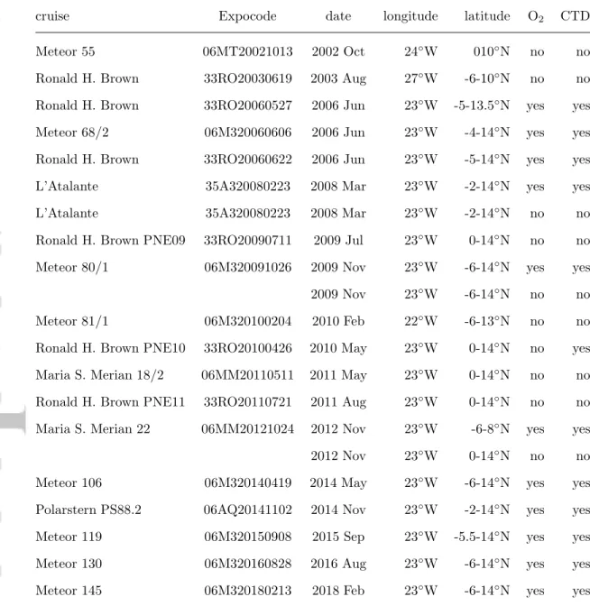
(2004) investigated the dynamics of the SEUC, the southern counterpart of the NEUC in
111
the Atlantic. Their model results show that the Eliassen-Palm flux associated with the
112
propagation of Tropical Instability Waves (TIWs) can be one possible driver of such zonal
113
currents. Other model studies in the Pacific suggest that the oceanic jets are pulled by the
114
upwelling within domes in the eastern basin or by the eastern boundary upwelling (Furue
115
et al., 2007, 2009; McCreary et al., 2002).
116
The NEUC is a weak and highly variable current. Its observed core velocity varies
117
from below 0.1 m s−1 (Brandt et al., 2006) to over 0.3 m s−1 (Urbano et al., 2008). In
118
ship sections the NEUC is likely to be biased by the high mesoscale activity present in
119
the tropical Atlantic (e.g. Goes et al., 2013; Weisberg & Weingartner, 1988). Furthermore,
120
estimates of NEUC transport are difficult because a clear separation of the current cores
121
of the NEUC and North Equatorial Countercurrent (NECC) above is not possible (Fig.
122
2a). Observational estimates range from 2.7 Sv to 6.9 Sv in meridional ship sections taken
123
between 38◦W and 35◦W (Bourl`es et al., 2002, 1999; Schott et al., 2003, 1995; Urbano et al.,
124
2008). Another problem is that some transport estimates from observations only cover part
125
of the NEUC, as for example Brandt et al. (2006) calculated zonal current transports from
126
a mean ship section along 26◦W. They found a transport of only 0.8 Sv for the eastward
127
flow in the region of the NEUC along 26◦W, but only covered the flow south of 5◦N.
128
Goes et al. (2013) used a synthetic method to estimate the NEUC transport between
129
30◦W and 23◦W. They combined expendable bathythermograph (XBT) temperature with
130
altimetric sea level anomalies to derive NEUC location, velocity and transport. In the po-
131
tential density layers of 24.5-26.8 kg m−3they found a NEUC transport varying from 2.3 Sv
132
during August to October to up to 5.5 Sv during May and June. The core position of the
133
NEUC in the synthesis product varies between 4.5◦N and 5.5◦N and exhibits a semiannual
134
cycle with minima in April and September and maxima in August and December. Their
135
estimated NEUC core velocities were highest in June (above 0.3 m s−1) and lowest during
136
boreal fall (below 0.2 m s−1). In a model study, H¨uttl-Kabus and B¨oning (2008) found a
137
clear seasonal cycle of the NEUC at 35◦W and 23◦W with maximum NEUC transports (4.5-
138
7.0 Sv) between May and June, and minimum transports (1.2-4.2 Sv) between September to
139
October. They found a westward propagation of the seasonal cycle consistent with annual
140
Rossby wave patterns (B¨oning & Kr¨oger, 2005; Brandt & Eden, 2005; Thierry et al., 2004).
141
In ship sections the NEUC shows no clear seasonal cycle. Four transport estimates
142
exist between 35◦W and 38◦W during boreal spring from 1993 to 1996 (Bourl`es et al., 1999;
143
Schott et al., 1995). In the same depth range as in Goes et al. (2013) and H¨uttl-Kabus and
144
B¨oning (2008) they vary from 1.6 Sv to 3.6 Sv and the NEUC position varies between 3.5◦N
145
to 5.5◦N. For boreal fall there is one NEUC transport estimate of 2.5 Sv between 4◦N and
146
6◦N (Bourl`es et al., 1999). Note that especially during boreal summer and fall as well as
147
in the mean ship sections the NEUC and the NECC are difficult to distinguish (Bourl`es
148
et al., 2002, 1999; Brandt et al., 2006; Schott et al., 2003; Urbano et al., 2008). As the
149
NEUC is likely to be obscured by the high mesoscale activity (Goes et al., 2013; Weisberg
150
& Weingartner, 1988) the mean is uncertain and the seasonal cycle cannot be estimated
151
reliably from ship sections.
152
Only few studies have investigated the interannual variability of the NEUC. In a model
153
study H¨uttl-Kabus and B¨oning (2008) estimated an interannual variability of the seasonal
154
cycle of 2 Sv, which is almost as strong as the amplitude of the seasonal cycle (3 Sv). The
155
results of Goes et al. (2013) indicate an anticorrelation between NEUC transport variability
156
and the Atlantic Meridional Mode (AMM). The AMM is characterized by a meridional inter-
157
hemispheric gradient of sea surface temperature (SST) in the tropical Atlantic centered
158
around 5◦N (Nobre & Shukla, 1996). Important drivers of the AMM are wind-induced
159
evaporation and the wind-evaporation-SST (WES) feedback (Carton et al., 1996; Chang
160
et al., 2000). Initially high SSTs in the northern tropical Atlantic lead to a low sea level
161
pressure anomaly which causes cross equatorial sea surface wind anomalies blowing from
162
the southern towards the northern hemisphere. This strengthens the southeast trade winds,
163
increases evaporation and leads to a negative heat flux anomaly into the ocean in the
164
southern hemisphere, i.e. a reduction of SST here. In the northern hemisphere the trade
165
winds are weakened by the anomalous atmosphere flow, and less evaporation associated
166
with a positive heat flux anomaly into the ocean amplifies the initial warming here. This is
167
referred to a positive AMM. The negative AMM is associated with a warming and a cooling
168
in the southern and northern hemisphere, respectively.
169
Goes et al. (2013) hypothesized that changes in the meridional density gradient driven
170
by the AMM is a possible mechanism that can drive NEUC variability. They highlight the
171
inverse SST anomalies in the Guinea Dome region and in the equatorial Atlantic associated
172
with the AMM. This can alter the north-south density gradient in the NEUC region and
173
strengthen (negative AMM, increased density gradient) or weaken (positive AMM, decreased
174
density gradient) the NEUC core (Furue et al., 2007; Goes et al., 2013; McCreary et al.,
175
2002).
176
In summary, the interannual variability of the NEUC and its potential drivers are still
177
not fully understood. As the NEUC is suggested to act as an important oxygen supply
178
route towards the ETNA OMZ, it is crucial to understand possible mechanisms by which
179
the NEUC variability impacts the oceanic oxygen distribution. As observations are still too
180
sparse, we will use a state of the art ocean general circulation model (OGCM) in combination
181
with a conceptual model to study these mechanisms.
182
In this study we investigate the interannual variability of the NEUC and the associated
183
oxygen response in a state of the art OGCM and a conceptual model. The study aims to
184
improve (1) the understanding of oceanic processes that impact the mean distribution and
185
interannual variability of dissolved oxygen in the NEUC region and (2) the understanding
186
of discrepancies between simulated and observed NEUC variability and associated oxygen
187
changes. For our analysis we are using the output of the high-resolution OGCM TRATL01
188
(Duteil et al., 2014) in combination with an unique data set of 21 ship section along 23◦W
189
from 2002 to 2018. We utilize an algorithm developed by Hsin and Qiu (2012) to estimate the
190
NEUC position and intensity in both the observational data and the output of TRATL01.
191
To better understand the contradicting results between the observations and the TRATL01
192
output we extend our analysis with a conceptual model simulating an eastward current and
193
its westward return flow with an oxygen source at the western boundary following Brandt
194
et al. (2010).
195
2 Data and Methods
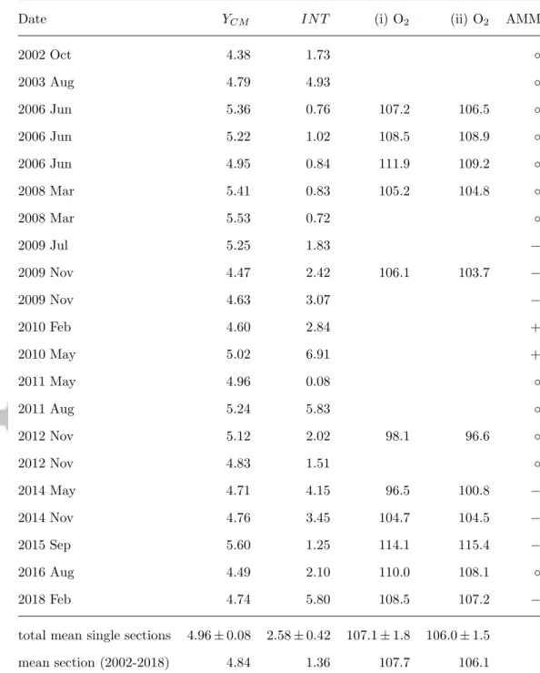
196
2.1 Observations
197
Velocity data of 21 ship sections along 23◦W obtained from 2002 to 2018 are used. For
198
13 and 11 of this sections also hydrographic and oxygen data are available, respectively. A
199
detailed overview of the cruises is shown in Table 1. All ship sections cover at least the
200
upper 400 m between 0◦ and 8◦N.
201
Velocity data are acquired by vessel-mounted and lowered Acoustic Doppler Current
202
Profilers (ADCPs). Vessel-mounted ADCPs (vm-ADCPs) are continuously recording ve-
203
locities throughout the section. The accuracy of 1 h averaged vm-ADCP data is better
204
than 2-4 cm s−1 (Fischer et al., 2003). Lowered ADCPs (l-ADCPs) are attached in pairs of
205
upward and downward looking instruments to a CTD (Conductivity-Temperature-Depth)
206
rosette and record velocities during CTD casts typically performed on a uniform latitude
207
grid with half-degree resolution. This enables velocity measurements throughout the whole
208
water column. The accuracy of full-depth l-ADCP velocity profiles is better than 5 cm s−1
209
(Visbeck, 2002). Hydrographic and oxygen data are obtained during CTD casts. The data
210
accuracy for a single research cruise is generally assumed to be better than 0.002◦C, 0.002
211
and 2µmol kg−1for temperature, salinity, and dissolved oxygen, respectively (Hahn et al.,
212
2017). The final ship sections and mean sections along 23◦W are obtained from the ob-
213
servational data as described in Brandt et al. (2010). First all velocity data are merged
214
accounting for their different accuracy and resolution. Then the velocity, hydrographic and
215
oxygen data are mapped on a regular grid (0.05◦ latitude×10 m) using a Gaussian inter-
216
polation scheme. All data are averaged at each grid point to derive the mean sections which
217
are smoothed by a Gaussian filter (horizontal and vertical influence (cutoff) radii: 0.05◦
218
(0.1◦) latitude and 10 m (20 m), respectively). For the mean velocity, temperature, salinity
219
and oxygen section the standard error in the NEUC region (100−300 m depth, 3◦−6.5◦N)
220
are 1.4 cm s−1, 0.12◦C, 0.01 and 3.4µmol kg−1, respectively.
221
2.2 High-resolution global ocean circulation model TRATL01
225
We are using the output of the global ocean circulation model TRATL01, in which a
226
1/10◦nest covering the tropical Atlantic from 30◦S to 30◦N is embedded into a global 1/2◦
227
model (Duteil et al., 2014). TRATL01 reproduces the tropical zonal jets more realistically
228
compared to a coarser resolution model, resulting in an improved representation of the
229
low oxygenated regions in the ETNA (Duteil et al., 2014). The model is based on the
230
Nucleus for European Modeling of the Ocean (NEMO) v3.1 code (Madec, 2008). The
231
thickness of its 46 vertical levels increases from 6 m at the surface to 250 m at depth. The
232
model is forced with momentum, heat and freshwater fluxes from the Coordinated Ocean-Ice
233
Reference Experiments (CORE) v2 data set for the time period from 1948 to 2007 (Griffies
234
et al., 2009). A simple biogeochemical model is coupled with the global ocean circulation
235
model. The biogeochemical model contains 6 compartments (dissolved oxygen, phosphate,
236
phytoplankton, zooplankton, particulate and dissolved organic matter). The parameter set
237
(e.g. phytoplankton growth rate, mortality, grazing) has been optimized to realistically
238
reproduce the oxygen and phosphate distribution in a global model (Kriest et al., 2010).
239
We are analyzing the monthly mean model output from 1958-2007. In TRATL01,
240
oxygen concentrations in the NEUC region (100−300 m depth, 3◦−6.5◦N, 45◦−15◦W) are
241
drifting on average by−0.5µmol kg−1yr−1 from 1958-2007; reaching an equilibrium state
242
would take several hundred years. The spurious drift is very strong in the first 30 years (144
243
% of the averaged drift). Therefore, the analysis of the oxygen variability is restricted to the
244
period 1990-2007 where the drift is only 11 % of the averaged drift. For the mean velocity,
245
temperature, salinity and oxygen section along 23◦W from 1990 to 2007 in TRATL01 the
246
standard errors in the NEUC region (100−300 m depth, 3◦−6.5◦N) are 1.02 cm s−1, 0.09◦C,
247
0.01 and 0.81µmol kg−1, respectively.
248
2.3 NEUC characterization
249
For both, TRATL01 and the observational data we calculate the central positionYCM
250
and along-pathway intensityIN T of the NEUC using the algorithm of Hsin and Qiu (2012).
251
YCM(x, t) = RZu
Zl
RYN
YS y u(x, y, z, t)dy dz RZu
Zl
RYN
YS u(x, y, z, t)dy dz (1)
252
253
IN T(x, t) = Z Zu
Zl
Z YCM+W YCM−W
u(x, y, z, t)dy dz (2)
254
wherey is latitude, xis longitude, uis zonal velocity, z is depth,t is time,Zu (Zl) is
255
upper (lower) boundary of the flow,YN (YS) is northern (southern) limit of the flow, and
256
W is the half mean width of the flow.
257
The advantage of this method is that the transport calculation follows the current core
258
avoiding artifacts if the current is meridionally migrating. In TRATL01 we choose the depth
259
of the 24.5 kg m−3 neutral density surface as the upper boundaryZu. This density surface
260
represents the upper boundary of the NEUC during boreal winter, the season when the
261
NECC is weak or not present and the NEUC can clearly be separated from the near-surface
262
flow. The lower boundary Zl is the depth of the 27.0 kg m−3 neutral density surface. A
263
half mean widthW of 2◦ is chosen for the NEUC. The integration is performed between
264
42◦W and 15◦W. For the integration of the observational data slightly different boundary
265
conditions are chosen to be consistent with the hydrographical conditions of the region. Zu
266
is the depth of the 24.5 kg m−3andZlthe depth of the 26.9 kg m−3neutral density surface.
267
The southern boundary is choosen asYCM−1.5◦and the northern boundary isYCM+ 1.0◦.
268
Note, if no hydrographic measurements are available for a single ship section, the neutral
269
density field derived from the mean hydrographic section is used.
270
2.4 Conceptual model
271
We are using a conceptual model to investigate the oxygen response to specific circu-
272
lation processes within the NEUC. It is based on the advection-diffusion model described
273
in Brandt et al. (2010) which simulates an eastward current and its westward return flows
274
with an oxygen source at the western boundary. The model equation (Eq. 3) used for all
275
simulations throughout the study reads:
276
∂C
∂t =−aOU R−u∂C
∂x −v∂C
∂y +kx
∂2C
∂x2 +ky
∂2C
∂y2 +kyFcorr
∂2Cbg
∂y2 +kzFcorr
∂2Cbg
∂z2 (3)
277
whereCis the dissolved oxygen concentration,aOU Rthe oxygen consumption, u and
278
v the zonal and meridional velocity components, respectively, kx and ky the zonal and
279
meridional eddy diffusivities, respectively,kz the vertical eddy diffusivity,Cbg the constant
280
large-scale background oxygen distribution, andFcorra correction factor to the background
281
oxygen curvature depending on the simulated oxygen concentration described below. The
282
oxygen concentration at the western boundaryC0 is held constant at 147µmol kg−1, which
283
is the mean oxygen concentration at the western boundary of the NEUC (γn= 26.5 kg m−3,
284
2.5◦−6.5◦N, 43◦-47◦W) derived from the MIMOC climatology (Schmidtko et al., 2017).
285
In the model, the following 7 terms on the right hand side determine the oxygen tendency
286
on the left hand side: (from left to right) (1) oxygen consumption, (2) zonal advection, (3)
287
meridional advection, (4) zonal eddy diffusion, (5) meridional eddy diffusion associated with
288
east- and westward jets and (6) meridional and (7) vertical eddy diffusion associated with
289
the large-scale oxygen distribution in the upper 300 m between 0◦N and 10◦N.
290
The model parameters are tuned to fit a region covering an eastward current and its
291
return flow between 2.5◦N (y= 0) and 6.5◦N (y=ly) from 45◦W (x= 0) to 10◦W (x=lx).
292
For the idealized background flow field we use the same definition of the streamfunction as
293
described in Brandt et al. (2010) and adjust it to fit the observations in the NEUC regions.
294
u=u0
lx−x lx cos
2π y ly
, v=−u0
2π ly
lxsin 2π y
ly
(4)
295
whereu0 is the amplitude of the zonal jets at the western boundary. For steady state
296
solutions, u0 is held constant, whereas for some interannual variability simulations u0 is
297
multiplied with a time varying sinusoid.
298
Two modifications of the Brandt et al. (2010) model are realized. (i) We are using a
299
constant, depth dependent oxygen consumption according to Karstensen et al. (2008), (ii)
300
we modify the model parameters to correspond to the conditions of the NEUC region.
301
(i) The oxygen consumption used here is defined as the logarithmic function as given
302
in Karstensen et al. (2008)
303
aOU R=c1+c2·e−λz (5)
304
(c1 =−0.5,c2= 12,λ= 0.0021). To avoid negative oxygen values, the consumption term
305
is switched off when oxygen concentrations fall below 2 µmol kg−1.
306
(ii) We fit our parameters to the 26.5 kg m−3neutral density surface which corresponds
307
to the core depth of the NEUC. A meridional and vertical eddy diffusion associated with the
308
large scale oxygen distribution is derived from observations, as well as a correction factor
309
for the background meridional diffusion as described below.
310
The NEUC is located in a region where oxygen concentrations are increasing equa-
311
torwards and decreasing polewards. Also in the vertical profile oxygen concentrations are
312
changing within the NEUC. To account for this background oxygen field we estimate a merid-
313
ional and vertical eddy diffusion associated with the meridional and vertical oxygen curva-
314
ture in the observation at 23◦W. We obtain the meridional eddy diffusion associated with
315
the meridional oxygen distribution (∂2∂yC2bg =Dy) similar to Brandt et al. (2010). We apply
316
a second-order fit to the observed oxygen distribution along the 26.5 kg m−3neutral density
317
surface at 23◦W between 0◦ and 10◦N which results inDy = 1.55·10−10µmol kg−1m−2.
318
The vertical eddy diffusion associated with the vertical background oxygen distribution
319
(∂2∂zC2bg =Dz) is estimated by calculating the curvature of the mean vertical oxygen profile
320
between 2.5◦N and 6.5◦N at 23◦W. We obtainDz= 0.0112µmol kg−1m−2for 130 m which
321
corresponds to the depth of the 26.5 kg m−3neutral density surface.
322
The correction factor for the background meridional diffusion is given as follows:
323
Fcorr=C0−C23W
C0−C1
(6)
324
whereC0is the oxygen concentration at the western boundary (147µmol kg−1),C1 is
325
the observed mean oxygen concentration along 23◦W between 2.5◦N and 6.5◦N (108µmol kg−1)
326
andC23W is the corresponding simulated value. This factor acts to damp changes of oxygen
327
due to the background eddy diffusivity depending on the meridional and vertical oxygen
328
curvature. That means ifC23W is higher (lower) thanC1 the oxygen supply because of the
329
background eddy diffusion decreases (increases).
330
The coefficients of the horizontal and the vertical eddy diffusion are chosen based on
331
previous observational studies. We use a vertical diffusivity ofkz= 10−5m2s−1(Banyte et
332
al., 2012; Fischer et al., 2012; K¨ollner et al., 2016). Hahn et al. (2014) suggested a meridional
333
diffusivity ky of 500−1400 m2 s−1 between 100-300 m depth. Globally, previous studies
334
suggest an anisotropy between zonal and meridional diffusivities with zonal diffusivity larger
335
than meridional (Banyte et al., 2013; Eden, 2007; Eden and Greatbatch, 2008; Kamenkovich
336
et al., 2009). Brandt et al. (2010) found thatky = 200 m2s−1 andkx= 2.5×ky (kx is the
337
zonal diffusivity) best fits the observations in the ETNA OMZ (∼400 m depth). Here, we
338
calculate the equilibrium state for differentky and kx. We found that a meridional eddy
339
diffusivity ofky= 800 m2s−1with no anisotropy (i.e. kx=ky) andu0= 0.055 m s−1results
340
in oxygen concentrations along 23◦W that best matches observations (Fig. S1a,c). In the
341
following we will refer to this simulation as SIM 1.
342
3 Results
343
The interannual variability of the NEUC and its impact on the oceanic oxygen distribu-
344
tion is investigated using ship observations along 23◦W and the output of TRATL01. First
345
we briefly validate and discuss the zonal velocity and oxygen sections along 23◦W TRATL01.
346
Then we present the results of the interannual variability of the NEUC in TRATL01 before
347
we focus on the oxygen response associated with NEUC variability. Finally, we present the
348
results of the conceptual model to understand the role of specific mechanisms.
349
3.1 Mean velocity and oxygen section along 23◦W
350
In the mean ship section along 23◦W, below the mixed layer, higher oxygen concentra-
351
tions locally coincide with the eastward flowing EUC, NEUC and nNECC at 0◦N, 4.5◦N and
352
8.5◦N respectively, whereas the westward flows centered at 2.5◦N and 6.5◦N are associated
353
with lower oxygen concentrations (Fig. 2a,c). The core of the ETNA OMZ with oxygen
354
concentrations of 40µmol kg−1 is located between 400 m and 500 m and between 9◦N and
355
13◦N. In the upper 250 m south of 6◦N, oxygen concentration are in general higher than
356
north of 6◦N. This is associated with the more energetic zonal flow in the near-equatorial
357
belt including the NEUC.
358
From the observed zonal velocity field the NEUC intensity (IN T, Eq. 2) and central
368
position (YCM, Eq. 1) are calculated and averaged in two different ways: (i) They are
369
calculated using the mean ship section. Here, the averaged NEUC intensity is 1.2 Sv and
370
the current is on average located at 4.9◦N. (ii) The estimates of the single ship sections
371
are averaged. This results in an average intensity of 2.6 ± 0.4 Sv and an averaged central
372
position of 5.0 ± 0.1◦N (Tab. 2). Method (ii), which results in higher values, is more
373
consistent with the method used for the model output.
374
Similar to the observations, oxygen concentrations along 23◦W in TRATL01 are in-
375
creased in the presence of eastward flow and decreased in the presence of westward flow
376
(Fig. 2b,d). The NEUC in TRALT01 is on average more than twice as strong as in the
377
observations and its core is located a bit further south. The mean NEUC intensity at 23◦N
378
(1990-2007) is 7.4 ± 0.3 Sv and its mean central position is 4.44 ± 0.03◦N. The model is
379
overestimating the strength and depth range of the NEUC and the nSEC whereas weaker
380
eastward current bands such as the NICC and the nNECC are not well represented by the
381
model.
382
In TRATL01 oxygen concentrations below the mixed layer are generally lower, the
383
oxygen minimum zone is located shallower, and the difference between local oxygen maxima
384
and minima is smaller compared to observations. The core of the OMZ in TRATL01 is
385
200 m shallower than in observations. Also the deep oxygen maximum at the equator is
386
not well represented in TRATL01. Although the NEUC is stronger, oxygen concentrations
387
within the NEUC region at 23◦ W (100−300 m depth, 3◦−6.5◦N) are lower in TRATL01
388
(93.4±0.8µmol kg−1) compared to observations (106.0±1.5µmol kg−1).
389
Different mechanisms seem to dominate the NEUC mean state in observations and in
390
TRATL01. Not only the NEUC is very strong in TRALT01, but also the nSEC south of it.
391
One explanation for that can be a too strong recirculation between nSEC and NEUC. In the
392
ship section from February 2018, a temporary recirculation between the nSEC and NEUC
393
seems to exist (black dashed rectangles in Fig. 1b,c). Here, the velocity maximum between
394
3◦N and 5◦N in the depth range of 50 m to 300 m is associated with rather low oxygen and it
395
is located above and south of the NEUC associated oxygen maximum. It is likely that this
396
eastward velocity maximum is a temporary recirculation of the nSEC which overlaps with
397
the actual NEUC flow. This results in lower oxygen values associated with higher eastward
398
NEUC velocities. An overestimation of this process by TRATL01 could result in the shown
399
discrepancies between model and observations. Strong recirculation between EUC, NEUC
400
and nSEC are also shown in other model studies such as H¨uttl-Kabus and B¨oning (2008).
401
In summary, distinct discrepancies exist between simulated and observed zonal veloci-
402
ties and oxygen concentration in the mean sections along 23◦W. A potential cause for the
403
differences in the mean state is an overestimation of the recirculation between nSEC and
404
NEUC in TRATL01. Nevertheless, we want to emphasize here that the horizontal oxygen
405
distribution is clearly improved in TRATL01 compared to coarser resolution models (Duteil
406
et al., 2014). How the erroneous representation of the mean state in TRATL01 affects the
407
NEUC and associated oxygen changes on interannual timescales will be investigated in sec-
408
tion 3.4. Before we focus on the oxygen response to the NEUC we investigate the variability
409
of NEUC transports and central position. In the next section we briefly study the seasonal
410
cycle of the NEUC in observations and in TRATL01.
411
3.2 Seasonal cycle of NEUC intensity (IN T) and central position (YCM)
412
In the previous section we found that on average the NEUC is too strong in TRATL01
413
but simultaneously shows a weaker oxygen maximum along 23◦W compared to observations.
414
We hypothesize that this might be due to an overestimation of the recirculations between
415
nSEC and NEUC in TRALT01. Here, we focus on the seasonal cycle of the NEUC in
416
observations and in TRATL01.
417
The NEUC transport estimates derived from the observational data are highly variable
418
and show no clear seasonal signal (Tab. 2 and black dots in Fig. 3a). This is in agreement
419
with previous observational results (Bourl`es et al., 2002, 1999; Brandt et al., 2006; Schott
420
et al., 2003, 1995; Urbano et al., 2008). The current is weak and likely to be obscured by
421
mesoscale activities (e.g. Goes et al., 2013; Weisberg & Weingartner, 1988) and interannual
422
variability (Goes et al., 2013; H¨uttl-Kabus & B¨oning, 2008). Even with this unique data set
423
of 21 ship sections, observations are still too sparse to identify a seasonal variability of the
424
NEUC.
425
In TRATL01, the NEUC shows a clear seasonal cycle. Along 23◦W, the NEUC reaches
432
its maximum intensity of 11.4 Sv in May and its minimum intensity of 3.9 Sv in November
433
(red line in Fig. 3a). Its central position shows a semiannual cycle with southernmost
434
positions in September and January and northernmost positions in May and November
435
(Fig. 3b). The semiannual cycle of NEUC central position is not visible at all longitudes
436
(Fig. 3d). The seasonal signal of NEUCIN T and YCM is propagating from the eastern
437
boundary towards the west (Fig. 3c,d). Highest standard deviations of NEUC transports
438
occur during May and June in the eastern basin and during July and August in the western
439
basin (black contours in 3c). Maximum standard deviation of NEUC transports seems to
440
be associated with the seasonal weakening of the NEUC.
441
The seasonal cycle of the NEUC in TRATL01 is in good agreement with previous
450
studies. H¨uttl-Kabus and B¨oning (2008) also found a more northward position and higher
451
transports between April and August and a more southward position and lower transports
452
between September and March in their model simulation. The seasonal cycle of NEUC
453
transport estimates in TRATL01 is also consistent with the synthesis product of Goes
454
et al. (2013). Similar to Goes et al. (2013), we found a semiannual cycle of the NEUC
455
central position along 23◦W, although the timing of maxima and minima is shifted by
456
up to 2 months. We found minima in September and January and maxima in May and
457
November, whereas in Goes et al. (2013) minima occur in September and March and maxima
458
in August and December. In general, the seasonal strengthening of the eastern NEUC in
459
TRATL01 seems to coincide with the northward migration of the Intertropical Convergence
460
Zone (ITCZ) and the shoaling of the thermocline in the eastern equatorial Atlantic (Xie &
461
Carton, 2004).
462
In summary, a seasonal and longer term variability of the NEUC in observations can
463
not be identified. In TRATL01 the NEUC shows a clear seasonal cycle which is in general
464
agreement with previous studies. This encourages us to study the interannual variability of
465
the NEUC in the next section.
466
3.3 Interannual variability of NEUC
467
The NEUC transport and central position vary on interannual to multidecadal timescale
468
in TRATL01 (Fig.4). However, TRATL01 is driven by CORE v2 wind forcing that is based
469
on NCEP winds. The CORE forcing as well as the NCEP wind is known to exhibit spurious
470
multidecadal wind variability (Fiorino, 2000; He et al., 2016; Hurrell & Trenberth, 1998).
471
We therefore focus on the interannual variability of the NEUC in TRATL01.
472
NEUC transport and central position show a positive correlation in TRATL01. To
473
analyze the correlation, we zonally averaged NEUCIN T andYCMfrom 42◦W to 15◦W and
474
removed the seasonal cycle from 1958 to 2007 (blue lines in Fig. 4). To better understand the
475
role of interannual variability of the NEUC, we applied a 1-to-5-years band-pass Butterworth
476
filter to IN T and YCM (black lines in Fig. 4). Higher NEUC transports are generally
477
associated with a more northward position of the NEUC and vice versa with a significant
478
positive correlation between the band-pass filtered time series ofR= 0.33.
479
Previous studies suggest the upwelling in the Guinea Dome and along the Northwest
483
African coast in the ETNA as a possible driver of the NEUC (Furue et al., 2007, 2009) and
484
that changes in the wind field can impact the upwelling which in turn leads to changes in
485
the NEUC (Goes et al., 2013). To investigate this connection we perform a linear regression
486
of the band-pass filtered NEUCIN T onto the wind stress curl using monthly time series
487
regressed at lag 0 (Fig. 5). On interannual time scales, the wind stress curl explains up
488
to 40 % of the NEUC variability. Maximum positive correlation (R = 0.6) is found in
489
the eastern basin of the tropical North Atlantic between 2◦N and 8◦N and in the western
490
basin of the tropical South Atlantic between 0◦ and 8◦S. This large scale wind pattern may
491
not only impact the strength of the NEUC, but also effect the basin wide circulation. We
492
therefore regressed the wind stress curl on the NEUC and calculate the anomalous Sverdrup
493
streamfunction from the derived slopebtimes a unit transport of 1 Sv.
494
During a strong (weak) NEUC the derived anomalous Sverdrup streamfunction is asso-
495
ciated with a westward (eastward) velocity anomaly between 8◦N and 10◦N and an eastward
496
(westward) velocity anomaly just south off the equator (Fig. 5). At the western boundary
497
the closure of the anomalous Sverdrup streamfunction would result in a southward (north-
498
ward) and northward (southward) velocity anomaly north and south of the equator, respec-
499
tively. Between 40◦W and 10◦W just north of the equator the wind stress curl anomaly
500
leads to an anomalous northward (southward) Sverdrup transport. To further investigate
501
the relationship between the NEUC and the large scale wind field we perform a composite
502
analysis regarding the wind and SST field during strong and weak NEUC transports.
503
The band-pass filtered time series of NEUCIN T is used to define years of strong and
509
weak NEUC flow. As threshold 0.6 times its standard deviation is chosen (green line in
510
Fig. 6a). Then composites of SST and the wind field are calculated for years of strong
511
and weak NEUC transports (Fig. 6b,c). The composites show an inter-hemispheric SST
512
gradient with opposite sign for strong and weak NEUC transports. Associated are wind
513
anomalies pointing from the colder hemisphere towards the warmer hemisphere. These are
514
the characteristics of the AMM as described in the introduction. The interannual NEUC
515
variability is negatively correlated with the AMM. A positive AMM is associated with a
516
weaker and more southern NEUC, and the negative AMM is associated with a stronger and
517
more northern NEUC.
518
The anomalous inter-hemispheric winds during an AMM event link the interannual
525
variability of the NEUC to the AMM. Associated with a positive (negative) AMM event
526
is a negative (positive) wind stress curl anomaly along the equator and just north of it
527
east of 20◦W (Foltz & McPhaden, 2010b; Joyce et al., 2004). We find a similar wind
528
pattern for weak and strong NEUC, respectively (Fig. 5). The large-scale wind pattern
529
does not only effect the NEUC flow but also effects the basin-wide Sverdrup circulation in
530
the tropical Atlantic (Fig. 5). The anomalous northward Sverdrup transport between 40◦W
531
and 10◦W just north of the equator might impact the recirculation between the NEUC and
532
the nSEC. Furthermore, along the Northwest African coast south of 15◦N, we find alongshore
533
wind stress that act to weaken (strengthen) coastal upwelling during weak (strong) NEUC
534
transports (Fig. 6).
535
In summary, in TRATL01 the interannual variability of the NEUC is linked to the
536
AMM, likely due to its associated large-scale wind anomalies. Consistent with the results
537
of Goes et al. (2013), we find a strengthening and a more northward position of the NEUC
538
during negative AMM events and vice versa. The anomalous wind stress curl additionally
539
impacts the Sverdrup circulation between 10◦S and 10◦N. The response of oxygen to the
540
interannual changes of the NEUC in TRATL01 is investigated in the next section.
541
3.4 NEUC impact on oxygen
542
On interannual time scales the NEUC variability is linked to the AMM in TRATL01.
543
During positive AMM events, the NEUC transports are weaker and the current core is
544
displaced towards the south. During negative AMM events, the NEUC is stronger and
545
displaced towards the north. In this section we investigate the impact of the interannual
546
NEUC variability on oxygen. Brandt et al. (2010) suggest that weaker NEUC transports
547
lead to lower oxygen concentrations at 23◦W due to a weaker advection of oxygen-rich water
548
masses from the western boundary. Consequently, we expect lower oxygen concentrations
549
after positive AMM events and vice versa. The observational data show no clear connection
550
between oxygen concentration, NEUC transports and the AMM (Fig. S2). We will therefore
551
focus on the interannual variability of oxygen in TRATL01.
552
In TRATL01 the oxygen variability is analyzed along three characteristic neutral den-
553
sity (γn) surfaces of the NEUC. We choose the 25.5 kg m−3 surface for the upper part of
554
the NEUC, the 26.5 kg m−3surface for the central part of the NEUC, and the 26.9 kg m−3
555
surface for the lower part of the NEUC (Fig. 2). The mean oxygen concentrations and
556
horizontal velocities along all three γn surfaces of the period 1990 to 2007 are shown in
557
Figure 7. Along the upperγn surface in the area of the nSEC and NEUC low oxygen con-
558
centrations exist (Fig. 7a). Interestingly, minimum oxygen concentrations are found in the
559
western basin in the area of the nSEC supplying the eastward flow within the NEUC. This
560
suggests that the water masses in the upper NEUC in TRATL01 are only weakly connected
561
to the oxygen-rich waters in the western boundary and are instead provided largely out of
562
the recirculation between NEUC and nSEC. A possible mechanism causing the low oxygen
563
values along the 25.5 kg m−3 surface close to the western boundary might be a too weak or
564
inexistent intermediate current system in TRATL01. This would lead to a too low ventila-
565
tion at depth which again can result in an upward flux of low-oxygen waters towards the
566
surface due to either diapycnal mixing or vertical advection within the subthermocline cells
567
(Perez et al., 2014; Wang, 2005).
568
Along the 26.5 kg m−3 surface oxygen concentration are high in the western basin and
569
low in the eastern basin (Fig. 7b). At the northern flank of the NEUC and north of it a
570
tongue of high oxygen concentrations spreads towards the east. At the southern flank of
571
the NEUC and within the nSEC a tongue of low oxygen spreads towards the West. The
572
mean horizontal current field in combination with the oxygen concentrations indicates that
573
the NEUC in TRATL01 is partly supplied by water masses from the western boundary
574
and partly by water masses from the nSEC. This supports our previous hypothesis that
575
in TRATL01 a constant recirculation between nSEC and NEUC superimposed on a mean
576
eastward current results in a strong NEUC flow that is associated with low oxygen levels,
577
as it is supplied by the oxygen-poor water masses out of the nSEC.
578
At the lower part of the NEUC (26.9 kg m−3surface) a tongue of high oxygen concen-
579
tration centered at the NEUC spreads from the western to the eastern basin (Fig. 7c). Here,
580
the ventilation of the NEUC by the western boundary seems to dominate the water supply
581
of the NEUC with only weak recirculation occurring along the eastward path of the NEUC.
582
Note that eastward flow of waters with higher oxygen concentrations associated with the
583
NEUC reaches the eastern boundary north of 6◦N.
584
To investigate interannual variability of oxygen in TRATL01 the seasonal cycle is re-
588
moved from the oxygen field and a 5-years high-pass Butterworth filter is applied to the
589
annual averaged oxygen anomalies. Similar to the SST and wind stress analysis, composites
590
of oxygen and horizontal velocity for strong and weak NEUC transports are calculated (Fig.
591
8). We now focus on the oxygen variability along the 26.5 kg m−3 surface representing the
592
core depth of the NEUC in TRATL01.
593
At a first glance, the oxygen anomalies associated with the NEUC variability in TRATL01
594
appear to be counterintuitive. Along the 26.5-isopycnal during years of weak NEUC, pos-
595
itive oxygen anomalies exist along the NEUC path with a connection to the southwestern
596
boundary (Fig. 8a). For years of strong NEUC flow, negative oxygen anomalies occur along
597
the NEUC path instead (Fig. 8b). This is the opposite of what we would have expected
598
taken into account the mean velocity and oxygen fields along 23W.
599
Again, a too strong recirculation between the nSEC and NEUC might explain the oxy-
600
gen pattern in TRALT01. The composites analysis shows that during weak (strong) NEUC
601
flow, also the nSEC is weak (strong) and is transporting less (more) oxygen-poor water to
602
the western basin (Fig. 8). Associated is a weaker (stronger) than normal recirculation
603
between NEUC and nSEC and the NEUC is supplied by less (more) oxygen-poor water
604
from the nSEC. Additionally a weak (strong) nSEC is transporting less (more) oxygen-poor
605
water to the western basin. Positive (negative) oxygen anomalies develop in the western
606
basin, which may be then advected by the NEUC towards the east.
607
In the oxygen composites, anomalies occur in the entire tropical North Atlantic which
612
might be associated with the detected large-scale wind anomalies during anomalous NEUC
613
transports. For example, weak negative (positive) oxygen anomalies exist along the western
614
boundary during strong (weak) NEUC phases and cover a depth range of 50 m to 450 m
615
depth. These oxygen anomalies are associated with weak meridional velocity anomalies that
616
act to weaken (strengthen) the NBC and its return flow. This pattern could be related to the
617
closure of the Sverdrup circulation at the western boundary (Fig. 5b). The wind-field during
618
strong (weak) NEUC and negative (positive) AMM events acts to weaken (strengthen) the
619
NBC just north of the equator so that less (more) oxygen-rich water might be supplied there.
620
Furthermore negative (positive) oxygen anomalies during strong (weak) NEUC flow exist
621
also north of 7◦N. Here, we find westward (eastward) velocity anomalies in the anomalous
622
Sverdrup streamfunction at about 8◦N that are also visible in Figure 8. This westward
623
(eastward) velocity anomaly act to weaken (strengthen) the nNECC which again could
624
explain the oxygen anomalies there.
625
In contrast to our expectations, the NEUC strength and the oxygen concentrations
626
along its flow path are negatively correlated on interannual timescales in TRATL01. To
627
get a rough estimate of how much of the oxygen variability can be explained by the NEUC
628
variability we perform a lagged linear regression of oxygen on NEUC INT for the 1-5 years
629