Carl von Ossietzky Universität Oldenburg

(1)

Carl von Ossietzky Universität Oldenburg

Masterstudiengang Biologie

MASTERARBEIT

Fin whale (Balaenoptera physalus) distribution modelling in the Nordic Seas & adjacent waters

Vorgelegt von Diandra Düngen

Externer Betreuer: Dr. Ahmed El-Gabbas

Betreuender Gutachter: Prof. Dr. Helmut Hillebrand Zweiter Gutachter: Elke Burkhardt

Oldenburg, den 24.09.2019

(2)

SUMMARY

Understanding the dynamics of cetacean distribution in ecologically vulnerable regions is essential to interpret the impact of environmental changes on species ecology and ecosystem functioning.

Species distribution models (SDMs) are helpful tools linking species occurrences to environmental variables in order to predict a species’ potential distribution. Studies on baleen whale distribution are comparably rare in polar regions, mainly due to financial or logistic constraints and habitat suitability models are scarce. Using SDMs, this master thesis aims at identifying areas of suitable habitats for fin whales (Balaenoptera physalus) in the Nordic Seas during summer. A further aim is to identify important environmental variables that potentially drive the species’ distribution.

Opportunistic data were collected during ten RV Polarstern cruises from 2007 to 2018 during summer months (May to September) along with complementary opportunistic data from open source databases. Environmental covariates were chosen based on ecological relevance to the species, comprising both static and dynamic variables. MaxEnt software was used to model fin whale distribution, with presence-only data as a function of carefully chosen environmental covariates. This master thesis is one of the first studies to use SDMs to model suitable habitats of fin whales in the Arctic Ocean and revealed a link of the occurrence of fin whales to specific environmental variables. Most contributing variables were distance to shore and distance to sea ice edge, suggesting both static and dynamic variables to have an impact on habitat suitability in the Arctic Ocean. Four other environmental variables, namely bathymetry, slope, variability of sea surface temperature and mean salinity at 100 m depth were shown to also have an impact. Areas of high suitability were pronounced around the southwestern and -eastern side of Svalbard, as well as on the northern tip of Norway and southern East Greenland. These results generally demonstrate the effective use of SDMs to predict species distribution in highly remote areas, constituting a cost- effective method for targeting future surveys and prioritizing the limited conservation resources.

Results can be applied in a variety of purposes, such as designing marine protected areas, guiding seismic surveys and support the further use of opportunistic data in research.

(3)

ZUSAMMENFASSUNG

Die Dynamik der Verteilung von Walen, insbesondere innerhalb ökologisch sensibler Regionen, ist essentiell um Einfluss von Umweltveränderungen auf die Ökologie der Spezies zu verstehen.

Artenverteilungsmodelle, im Folgenden Species Distribution Models (SDMs) genannt, sind hilfreiche um Umweltparameter und Artenaufkommen verknüpfen zu können. Dies geschieht um räumliche (oder zeitliche) Verteilungen einer Art darzustellen. Es gibt vergleichsweise wenige Studien, die sich mit Bartenwalen in den Polarregionen befassen. Dies ist haupstächlich auf finanzielle und/oder logistische Restriktionen zurückzuführen. Auch durch die SDMs produzierten, sogenannten Habitateignungs-Modelle (Habitat Suitability Models), sind in diesen Gebieten vergleichsweise selten. Diese Masterarbeit zielt darauf ab, unter Verwendung von SDMs, geeignete Habitate für Finnwale (Balaenoptera physalus) im arktischen Sommer zu erkennen. Ein weiteres Ziel ist es, wichtige Umweltparameter, die der Verteilung der Wale zugrunde liegen, zu identifizieren. Opportunistische Daten wurden während zehn wissenschaftlichen Expeditionen der RV Polarstern, von 2007 bis 2018, innerhalb der Sommermonate (Mai bis September) erhoben.

Ergänzend dazu wurden opportunistische Daten von Open Source Datenbanken verwendet. Die Umweltparameter wurden bezüglich der ökologischen Relevanz der Art ausgewählt. Sie umfassen sowohl statische, als auch dynamische Variablen. Zur Modellierung der Finnwalverteilung wurde die Software MaxEnt gewählt, wobei aussschließlich Präsenzen als Funktion der ausgewählten Umweltparameter dienten. Diese Masterarbeit ist eine der ersten Studien, welche SDMs verwendet, um geeignete Habitate in der Arktis zu modellieren. Im Verlauf dieser Studie konnte ein Zusammenhang zwischen der Verteilung von Finnwalen und spezifischen Umweltparamentern hergestellt werden. Den größten Beitrag zur Verteilung der Finnwale steuerten hierbei die Distanz zur Küste, sowie die Distanz zur Eisgrenze bei. Vier weitere Umweltparameter, Bathymetrie, Hang, Abweichung der Wasseroberflächentemperatur, sowie die Salinität in einer Tiefe von 100 Metern, hatten ebenfalls Einfluss auf die Habitateignung. Besonders geeignete Gebiete fanden sich südwestlich bis -östlich vor Spitzbergen, an der nördlichen Spitze von Norwegen und dem südlichen Ost-Grönland. Die Ergebnisse demonstrieren den effektiven Gebrauch von SDMs, um Artenverteilung in abgelegenen Gebieten voraussagen zu können und stellen somit eine erschwingliche Methode für zukünftige Untersuchungen dar. Desweiteren können sie z.B. auf die Gestaltung von Meeresschutzgebieten, die Anleitung seismischer Untersuchungen oder der Förderung des weiteren Gebrauchs opportunistischer Daten in der Wissenschaft angewendet werden.

(4)

INDEX OF FIGURES

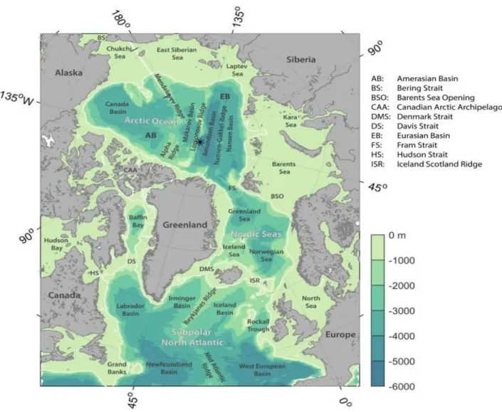
Fig. 1: Bathymetry of the Arctic Ocean and subpolar North Atlantic derived from the ETOPO2 database in 2-minute resolution. The white contour indicates the 500 m isobaths (Source: Horn 2018). ... 2

Fig. 2: (a) Exemplary spatial autocorrelation ranges of the environmental variables and (b) corresponding spatial blocks (Source: Valavi et al. 2018). ... 12

Fig. 3: The study area, covering N60° - N81° and W45° - E55°, including Svalbard and Iceland ... 14

Fig. 4: Correlation plot of all variables. Blue is depicting a positive, red a negative correlation, the intensity of shading and size of the circles is indicating the intensity of correlation. ... 19

Fig. 5: Spatial blocks for model versions with and without duplicates... 20

Fig. 6: Prediction maps of modelduplicates and modelnoduplicates. Habitat suitability ranges from 0 (blue; low) to 1 (red; high). ... 24

Fig. 7: Mean prediction map of the four cross-validated folds of modelduplicates and the according standard deviation. Habitat suitability ranges from 0 (blue; low) to 1 (red; high). ... 25

Fig. 8: Mean prediction map of the four cross-validated folds of modelnoduplicates and the according standard deviation. Habitat suitability ranges from 0 (blue; low) to 1 (red; high). ... 25

Fig. 9: Jackknife of regularized training gain for the full modelduplicates. Green indicates model performance without respective variable, blue indicates model performance with only variable. Red indicates model performance when all variables were used. ... 26

Fig. 10: Jackknife of regularized training gain for the full modelnoduplicates. Green indicates model performance without respective variable, blue indicates model performance with only variable. Red indicates model performance when all variables were used. ... 27

(5)

Fig. 11: PI for all EVs of the modelduplicates in a descending order. Dots resemble the full model, while bars indicate the mean PI of all four models. Error bars represent the standard deviation of PI. The solid horizontal line indicates a threshold of 6 below which EVs were of low interest. ... 28

Fig. 12: Permutation importance for all EVs of modelnoduplicates, in a descending order. Dots resemble the full model, while bars indicate mean PI values of all four model. Error bars represent the standard deviation of PI. The solid horizontal line indicates a threshold of 6 below which EVs were of low interest. ... 29

Fig. 13: Response curves for distance to shore (left) and sea ice edge (right). Ticks on the upper axis represent values at occurrences, while ticks on the lower axis represent values at background locations.

Number after model name indicates the permutation importance of the respective variable. ... 31

Fig. 14: Response curves for bathymetry (left) and slope (right). Ticks on the upper axis represent values at occurrences, while ticks on the lower axis represent values at background locations. Number after model name indicates the permutation importance of the respective variable. ... 32

Fig. 15: Response curves for salinity at 100 meters depth (left) and variability of sea surface temperature (right). Ticks on the upper axis represent values at occurrences, while ticks on the lower axis represent values at background locations. Number after model name indicates the permutation importance of the respective variable. ... 33

Fig. 16: Main circulation and water masses in the Barents Sea. The mean ice edge, using 15% (solid) and 40% (dashed) ice concentration, in September (black) and the Polar Front (grey) (Source: Johannesen et al.

2012). ... 35

(6)

INDEX OF TABLES

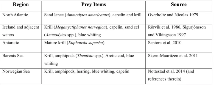
Table 1: Prey sources of fin whales in different parts of the Nordic Seas ... 7

Table 2: Covariates, source and time frame of raw data, * indicates temporal resolution, ** spatial resolution ... 17

Table 3: Overview of transformations and VIF of final EVs used in the model, sd = standard deviation, m

= mean ... 18

Table 4: Overview of the settings for modelduplicates and modelnoduplicates ... 21

Table 5: Niche overlap (prediction congruence) between predictions of each pair of the four cross-

validated models of modelduplicates ... 30

Table 6: Niche overlap (prediction congruence) between predictions of each pair of the four cross-

validated models of the modelnoduplicates ... 30

(7)

1. INTRODUCTION

Many whales, including fin whales (Balaenoptera physalus), are known to occur in high numbers in the North Atlantic Arctic throughout summer months (Heide-Jørgensen et al. 2003, Heide- Jørgensen et al. 2007, Mikkelsen et al. 2007, Heide-Jørgensen et al. 2008, Heide-Jørgensen et al.

2010, Laidre et al. 2010, Storrie et al. 2018). Unfortunately, several centuries of commercial whaling have reduced many cetacean populations to acritical level (Clapham et al. 1999, Roman and Palumbi 2003). By now, some are still endangered, while others are close to extinction (Clapham et al. 1999, Kraus et al. 2005, Schipperet al. 2008). Immense changes in abundance and distribution of large whales due to extensive hunting had significant impacts on the environment as well (Hacquebord 1999, Kruse 2016). Many of the species are recovering, though this is happening during a time of rapid environmental change so that an establishment of new distributional patterns is possible (see Storrie et al. 2018 and references therein). Furthermore, ship strikes, and alterations of prey availability are potential drivers of an observed decline in fin whale abundance in some parts of the North Atlantic (Schleimer et al. 2019). The investigation of cetacean habitat use and underlying oceanographic factors therefore is of particular importance. Especially due to baleen whales specialized diets (e.g. blue whales (Balaenoptera musculus)) and foraging strategies (such as in minke (Balaenoptera acutorostrata) or humpback whales (Megaptera novaeangliae)), rorqual whales may have a lower capacity for adaptation (Hain et al. 1982, Lynas and Sylvestre 1988, Hoelzel et al. 1989, Weinrich et al. 1992). They could, therefore, be more vulnerable to anthropogenic changes in the marine environment than other species (Kovacs and Lydersen 2008). In that sense, it is important to understand the relationship between whales and their environment at various temporal and spatial scales to assess potential ecosystem-level effects in response to changing environmental conditions (Hátún et al. 2009).

1.1. The Nordic Seas Ecosystem

The Arctic is a Mediterranean Ocean, consisting mainly of the Arctic Ocean and the Nordic Seas.

It covers the main parts of the Barents-, Greenland- and Norwegian Sea (Fig. 1).

(10)

1.1.1 The Nordic Seas

The Arctic Ocean is the northernmost part of the Arctic, while the Nordic Seas comprise the southward connecting Greenland-, Norwegian- and Iceland Seas (Loeng and Drinkwater 2007, Campos and Horn 2018). The Arctic Ocean and Nordic Seas are connected via Fram Strait and the Barents Sea (Fig. 1) (Ingvaldsen and Leong 2009, Campos and Horn 2018). The Barents Sea, covering most of the study area, is a shelf sea with high productivity, low biological diversity and strong species interactions (Wassmann et al. 2006). As largely enclosed ocean, only two water masses enter from other oceans, the cooler, low-salinity Pacific Water and the warmer, high-salinity Atlantic Water. The Arctic Front separates Arctic from Atlantic Water, while the more northwestward Polar Front separates Polar and Arctic Waters, being a mixture of Atlantic and Arctic Water (Loeng and Drinkwater 2007, Ingvaldsen and Loeng 2009).

Fig. 1: Bathymetry of the Arctic Ocean and subpolar North Atlantic derived from the ETOPO2 database in 2-minute resolution. The white contour indicates the 500 m isobaths (Source: Horn 2018).

(11)

The Arctic has several unique physical characteristics amongst which are strong seasonality in light (large variations in light levels, with up to 24 hours of sunlight in summer and darkness in winter), cold overall temperatures with winter extremes, and the presence of extensive shelf seas around a deep central ocean basin (Loeng and Drinkwater 2007, Kovacs et al. 2011). Of particular importance is the accumulation of large biomass – total mean annual primary production rate is 80 to 90 g C / m² – either through seasonally restricted and intense blooms or by local accumulation of biomass through advection at the Arctic continental shelves (Loeng and Drinkwater 2007, Laidre et al. 2010). With the annual retreat of winter sea ice, an enormous phytoplankton bloom is triggered based on drastic increases in sunlight, which by retreat of the ice sheet reaches the sea surface. This results in high densities of zooplankton and lower trophic level foraging fish, which again attracts large numbers of top marine predators (Heide-Jørgensen et al. 2007). Seasonal sea ice in the Barents Sea typically forms in March / April (max. coverage) (Loeng and Drinkwater 2007). Main currents in the Arctic run eastwards across the southern part of the Barents Sea, while in the northern parts, they run westwards (Ingvaldsen and Leong 2009, Wekerle et al. 2017). The North Atlantic Current splits into two branches, one entering the Arctic Ocean through the Barents Sea (North Cape Current), the other through Fram Strait (West Spitsbergen Current) (Wekerle et al. 2017, Campus and Horn 2018).

1.1.2 Climate Change

Climate in the Arctic is highly dynamic, affecting many aspects of this ecosystem. The warming atmosphere supports an early sea ice melt during summer and inhibits sea ice formation during winter, which leads to an overall reduced sea ice coverage and thus a reduced albedo (Pistone et al.

2014). This consequently leads to an increase in absorption of solar radiation, which again provides extra heat to the ocean that can initiate sea ice melt from below (Horn 2018). Besides this positive feedback loop, sea ice retreating earlier in spring and advancing later in fall leads to longer summers (Laidre et al. 2015). In the Greenland- and Barents Sea (and many other parts of the Arctic), the time of fall sea ice is negatively correlated with the time of spring ice retreat (Laidre et al. 2015).

The recent loss rate of Arctic sea ice is even faster than predicted by climate models (Stroeve et al.

2012), where summer sea ice extent has decreased by more than 40 % in recent decades (Overland and Wang 2013). Beyond that, sea ice loss is most likely to continue for several decades, even if emissions of greenhouse gases were limited immediately (Overland and Wang 2013).

(12)

Changes in temperature and decreasing sea ice coverage are expected to cause changes in productivity and energy cascades throughout the ecosystem (Parkinson et al. 1999, Heide- Jørgensen et al. 2007), eventually affecting cetaceans depending on this region (Derville et al.

2019). The decrease in sea ice coverage will most likely further increase anthropogenic activities in polar regions, as sea ice has previously been one of the limiting factors for accessing high latitudes (Gjosaeter et al. 2009). Already, anthropogenic activities have increased in West Greenland, including oil-, gas- and mineral exploration as well as tourism and whaling (Gjosaeter et al. 2009, Simon et al. 2010). This can affect fin whales, as they are the most commonly reported species to be involved in vessel collisions (Schleimer et al. 2019 and references therein).

1.1.3 Arctic Ecosystem

The Nordic Seas are home to a variety of species. Fish composition in the Norwegian Sea is dominated by pelagic species such as herring (Clupea harengus) and blue whiting (Micromesistius poutassou), whereas in the Barents Sea pelagic species (e.g. capelin, herring and Arctic cod (Boreogadus saida) and demersal species (like Atlantic cod (Gadus morhua) and haddock (Melanogrammus aeglefinus)) occur (Loeng and Drinkwater, 2007). Zooplankton community is dominated by copepods, mainly Calanus spp., but other important zooplankters also exist, including amphipods (especially Themisto spp.) and euphausiids (e.g. Thysanoessa spp. in the Barents Sea and Meganyctiphanes spp. in the Norwegian Sea) (Melle et al. 2004). In the Norwegian Sea, Rey (2004) has provided a detailed description of the seasonal cycle of phytoplankton with low primary production in winter and early spring, and a homogeneous distribution of nutrients (Rey and Loeng 1985): Within this period, phytoplankton communities are mainly composed of small flagellates. When sea ice retreats in spring (March / April) and light levels and concentrations of nitrate increase, primary production is initiated. With the increase in stratification in May, diatom blooms develop. Chlorophyll levels tend to stay low due to zooplankton grazers and production decreases by summer. Due to wind mixing, small blooms still occur until autumn, though by October declining light levels finally limit primary production (Rey 2004). For the Barents Sea, processes seem to be similar, though time-lagged (Rey and Loeng 1985, Loeng and Drinkwater 2007). It is a home for a variety of resident marine mammal species, including polar bear (Ursus maritimus), seven pinniped- and five cetacean species (Kovacs et al. 2009). Additional to these residents, eight cetacean species migrate regularly to the Barents Sea (Kovacs et al. 2009).

(13)

Marine mammals in the Barents Sea display high diversity in distributional patterns: while some are associated with sea ice most of the year, others prefer pelagic, open waters (Kovacs et al. 2009).

Then again, others are confined to the more temperate and shallow coastal waters (Kovacs et al.

2009). Arctic shelf regions are important to top marine predators, which are (seasonally) seeking abundant food resources in this region. Some marine mammals, such as ringed seals (Phoca hispida), Atlantic walrus (Odobenus rosmarus rosmarus) and polar bears rely on sea ice for several reasons and are, therefore, directly related to sea ice conditions (Weslawski et al. 1988, Jay and Fischbach 2008, Freitas et al. 2009). As a result, there is potential for dramatic ecosystem shifts given the observed reduction in sea ice coverage, ice thickness, extent, and duration, as well as changes in current patterns and temperature due to climate change (Carmack and Wassmann 2006).

These physical changes alter biota in Arctic regions such as Svalbard, e.g. with boreal invertebrate and fish species displacing native Arctic species (Loeng and Drinkwater 2007, Fossheim et al.

2015, Dalpadado 2016, Gluchowska et al. 2016). Furthermore, the Arctic marine food web structure is altered by a general poleward shift of boreal generalists (Kortsch et al. 2015). The distribution of several fish species that are of importance for cetaceans such as the fin whale, is influenced by climate variability: e.g. cod, herring and blue whiting distribution shifts northward during extended warm periods and southward during cooler periods (Gjosaeter et al. 2009). The increase in primary (and secondary) production that goes hand in hand with climate change leads to an increased fish production through higher abundance and improved growing rates (Overholtz and Nicolas 1979, Payne et al. 1990, Loeng and Drinkwater 2007). During the past 30 years, substantial changes regarding prey sources have occurred in the Barents Sea, amongst others tremendous rises and falls of capelin and herring, the predominant pelagic shoaling fish in the area (Gjosaeter et al. 2009, Kovacs et al. 2009).

1.2. Mysticetes

The Mysticetes comprise three families: Balaenidae (the right whales), Eschrichtiidae (gray whales) and Balaenopteridae (rorqual whales). Each family employs a distinct feeding method of the type of suspension feeding and are specifically categorized as filter-, suction- or raptorial feeders (Werth 2000). Fin whales belong to the family Balaenopteridae. Compared to their body size, balaenopterids are rather shallow divers (Gaskin 1982, Hamilton et al. 1997, Panigada et al.

1999).

(14)

They grow up to 30 meters in length, with the up to 24 m fin whale being the second largest and fastest cetacean (Katona et al. 1993). In order to feed effectively, rorqual whales engulf large quantities of dense food patches - a method that is called gulping or ram filter-feeding (Bowen and Siniff 1999, Werth 2000, Kimura 2004). They filter prey out of the water using baleen, which are attached to the upper jaw (Wells et al. 1999). These vary in length, thickness and narrowness according to species. The anatomy features a fusiform body, with parallel running ventral throat grooves and a muscular, specialized tongue that enables gulping large quantities of prey (Lambertsen 1983, Orton and Brodie 1987, Hoelzel et al. 1989, Bowen and Siniff 1999). Prey abundant water masses are engulfed through rapid gulps and lunges after which the water is expelled while prey is held back by the baleen (Bowen and Siniff 1999, Werth 2000). Seasonal and annual variations in prey densities seem to play an important role in the aggregation of baleen whales and their foraging profitability (Piatt and Methven, 1992), as feeding is thought to be restricted to seasons and usually latitude-dependent (Clapham 2000, Stern 2009). Despite this, recent observations suggest that Mysticetes also forage during migration (Geijer et al. 2016 and references therein, Owen et al. 2017). Silva et al. (2019) provide strong hints that North Atlantic fin whales, migrating through central Atlantic waters, feed during winter or early spring in tropical and subtropical waters and that this strategy is more prevalent among migratory whales than is currently acknowledged. Further, feeding in winter appears common among the North Atlantic fin whales and may play a crucial role in determining their winter distribution (Silva et al. 2019).

Mysticetes feed on comparatively small prey, hence they need to address high densities of prey: It has been estimated that 1–2 tons of zooplankton per day has to be ingested in order to meet energetic requirements (Kenney et al. 1986). Prey densities above a certain threshold are thought to be required to facilitate efficient foraging (Piatt and Methven 1992). Within feeding grounds, their high mobility allows the active search for the most food abundant areas and/or the highest prey patch densities (Wells et al. 1999).

1.2.1 Fin whales

Fin whales are the fastest swimmers among all whales and are believed to be the deepest diving species of all Mysticetes (Bérubé and Aguilar 1998, Panigada et al. 1999).Morphologically striking features include the asymmetric coloration of the head, dark coloration on the left anterior third of the body and baleen, and white coloration on the right lower jaw.

(15)

The right anterior part of the body is less heavily pigmented than the left part (Tershy and Wiley 1992, Aguilar 2009). Group sizes can vary, though usually fin whales occur singly or in pairs (Edds and Macfarlane 1987). Fin whales are considered opportunistic feeders, foraging on krill and pelagic fish, potentially varying preferences according to prey availability (see Table 1 for details).

However, considerable variations in feeding activity were found, depending on locality, time of the season, and prey species (Nemoto 1957, 1959).

Table 1: Prey sources of fin whales in different parts of the Nordic Seas

Region Prey Items Source

North Atlantic Sand lance (Ammodytes americanus), capelin and krill Overholtz and Nicolas 1979 Iceland and adjacent

waters

Krill (Meganyctiphanes norvegica), capelin, sand eel (Ammodytes spp.), blue whiting

Rörvik et al. 1986, Sigurjónsson and Víkingsson 1997

Antarctic Mature krill (Euphausia superba) Santora et al. 2010

Barents Sea Krill, amphipods (Themisto spp.), Arctic cod, blue whiting

Skern-Mauritzen et al. 2011

Norwegian Sea Krill, amphipods, herring, blue whiting, capelin Nottestad et al. 2014 (and references therein)

Fin whales utilize an energetically expensive strategy of lunge feeding at depth upon encounters with suitable densities of prey (Croll et al. 2001, Acevedo-Gutierrez et al. 2002, Simard et al. 2002, Croll et al. 2005, Goldbogen et al. 2006, 2007). There might be two scale-dependent foraging strategies of fin whales in summer: the large-scale site fidelity for the persistent area of krill habitat or, at the mesoscale, the search for the most concentrated food areas characterized by high dynamics of oceanographic processes (Cotté et al. 2009).Fin whales are thought to feed in depths of 100 to 200 meters (Katona et al. 1993) and are known to regularly return totraditional feeding grounds over many years, though winter breeding grounds have not been identified yet (Aguilar 2009). Observations of fin whales together with high prey densities support conclusions from previous satellite tracking studies that fin whales move into high latitudes to feed (Heide Jørgensen et al. 2003), which is consistent with prior findings (Stevick et al. 2008). There has been evidence that some individuals stay throughout December (Heide-Jørgensen et al. 2003, Simon 2010) rather than only visiting in summer.

(16)

In the Barents Sea, fin whales were shown to inhabit southern areas in early summer but not later in the season, clearly demonstrating a seasonal shift in their distribution (Haug et al. 2002, Skern- Mauritzen et al. 2011). Further findings suggest changes in body fattening in Icelandic waters, potentially related to food availability (Lockyer 1986). Several environmental factors have been put into context with the occurrence of fin whales, including primary productivity, bathymetry, sea surface temperature and sea surface height (Forcada et al. 1996, Littaye 2004, Sirovic et al. 2004, Laran and Gannier 2008, Panigada et al. 2008, Sirovic et al. 2009, Stafford et al. 2009, Azzellino et al. 2012, Druon et al. 2012, Breen et al. 2016, Zerbini et al. 2016, Prieto et al. 2017). Recently, Iceland established a new, increased catch quota for fin whales, which has been set to 209 individuals and may pose a risk to these stocks¹ . Despite the initial recovery from historical whaling, models predict considerable declines in Atlantic fin whale stocks, as well as local extinctions by 2100 (Tulloch et al. 2018, 2019). Stocks of fin whales in Arctic waters are not comprehensively calculated, though a considerable amount of studies exists on stocks of different parts of the study area, amongst which there are Iceland, Norway and Jan Mayen, as well as Greenland and the Faroes (Pike et al. 2005, Vikingsson et al. 2009, Vikingsson et al. 2015). There seem to be at least 25,000 to 30,000 fin whales in the North Atlantic (Kovacs et al. 2009). It has been reported that the number of fin whales in the North Atlantic has steadily increased in the past years and potentially has already recovered by 2000, though it is unclear if this is due to recovery from past whaling or favorable environmental changes (Víkingsson et al. 2015). Fin whales, like many other cetaceans, cover a wide range on foraging grounds, as their distribution is predominantly governed by prey availability (Kovacs et al. 2009). As the impact of climate change on fin whales will likely occur via changes to their prey, it is important to monitor and model their distribution in the study area to guide appropriate conservational measures. It has been hypothesized that, as marine productivity increases with the progressing loss of seasonal sea ice cover, a northward spread of cetacean species from more temperate waters to Svalbard and the northern Barents Sea can be expected, as has been shown for grey whales (Moore et al. 2003, Kovacs et al. 2009). Changes in fish, benthos and primary production in the study area have already been detected and described (Moore et al. 2003, Overland et al. 2004, Qu et al. 2006, Arrigo et al.

2008).

1 www.phys.org/news/2019-02-iceland-whaling-quotas-falling-profits.html

(17)

1.3. Species Distribution Modelling

One major challenge to predict patterns of species occurrence is to identify mechanisms leading to the presence of a species in a specific spatial and temporal dimension (Verity et al. 2002). Species distribution modelling (SDM), also known as environmental niche modelling (ENM), can be a helpful tool that links the occurrence of certain species to environmental variables and then provides insight into potential species’ distribution. SDMs are statistical tools that estimate the relationship between species occurrences at field sites and the environmental characteristics of those sites (Franklin 2010). This is especially helpful in remote and limited-access areas, such as the polar oceans. One of the approaches commonly used to describe habitat requirements of a species, is by fitting niche- or distribution models and to use these to identify the potential distribution of the respective species by projecting onto geographical space (Robinson et al. 2011, Tyberghein et al. 2012). There are different approaches to model species distribution, including correlative (Pearson and Dawson 2003), coupled correlative and process-based models (Smolik et al. 2010), as well as mechanistic approaches (Kearney and Porter 2009). Correlative SDMs relate species occurrence data (presence-only or presence-absence) with environmental data of a specific area to explain and predict the species’ distribution. In contrast, mechanistic approaches use the physiological characteristic of a species to determine the range of environmental conditions within which the species can persist (Kearney and Porter 2009). Both approaches comprise the Grinnellian understanding of “environmental niche”, assuming the observed distribution of a species to be governed by its abiotic preferences, food requirements and/or microhabitat characteristics (Grinnell 1904). These approaches also vary in the kind of required data. In surveys, where sites are systematically researched and presence-absence or abundance of species is recorded, regression methods and their extensions, such as generalized linear models (GLMs), generalized additive models (GAMs) or regression trees may be used (Elith et al. 2011). For many regions though, such systematic surveys are not applicable, and accurate absence or abundance data cannot be obtained.

Depending on the species, absences are not easily determined (Wintle et al. 2015). In such cases, species occurrence data are often available in the form of opportunistic presence-only records in museum databases and online repositories (e.g. GBIF or PANGAEA)² (Elith et al. 2011).

Advantages of presence-only (or presence-background) records are the relatively easy accessibility compared to presence-absence or abundance data (Elith et al. 2006).

2https://www.pangaea.de/, https://www.gbif.org/

(18)

Intent and methods of presence-only data are often unknown though, leading to potential biases (Hijmans et al. 2000, Reese et al. 2005, Elith et al. 2006). Due to sampling design, taking account of potential bias is important. Here, duplicates were removed in order to avoid spatial sampling bias (Fourcade et al. 2012, El-Gabbas and Dormann 2018). Presence-only models are commonly implemented in terrestrial habitats, where their use has gained much intension over past years, whereas SDMs of marine species are comparatively rare, though interest in their application has increased (Redfern et al. 2006, Valavanis et al. 2008, Robinson et al. 2011). Potentially, the comparably easy access to satellite data, which are often the basis of environmental data, lead to an increased use of SDMs (Palialexis et al. 2011). Many novel modelling methods have been proposed to be applied to marine species (see Palialexis et al. 2011 and references therein). A few methods that use presence-only data exist, amongst which there is MaxEnt (Phillips et al. 2006, Phillips and Dudik 2008). MaxEnt estimates the most uniform distribution of the species, by contrasting the sampling points against many background locations randomly sampled from the study area, with implementation of some constraints (Phillips et al. 2004, Phillips et al. 2006). It takes a list of species presences (locations) as input, as well as a set of environmental variables (e.g. salinity or temperature) across a user-defined geographical space, which is divided into grid cells. MaxEnt extracts a sample of background locations (where presences are unknown), which then are contrasted against the presence locations (Merow et al. 2013). The probability distribution of the species is estimated in terms of maximum entropy, which is the distribution that is closest to uniform across the study area (Phillips et al. 2006). Environmental variables (or predictor variables or covariates; hereafter: "EVs") are independent factors that can describe niche requirements of a species can be relevant to habitat suitability (e.g. temperature, bathymetry). The selection of environmental variables is based on a priori knowledge of the important ecological drivers of the focal species (Austin 2007). Often, the final choice of environmental variables is governed by their availability, -and collinearity (Bombosch 2013, Zeng et al. 2016). Collinearity often leads to overfitted models, so good practise is to remove correlated variables in the modeling process (Zuur et al. 2010). Since becoming available in 2004, the use of MaxEnt has grown extensively for modelling species distributions (Elith et al. 2011) and it became open source in 2017 (Phillips et al. 2017). It has become a popular tool for studying species distribution, because it is user-friendly, while at the same time its predictive performance is consistently competitive with the highest performing methods and even outperforms other methods in predictive accuracy (Elith et al. 2006, Merow et al. 2013).

(19)

According to Austin (2002), it is desirable to fit nonlinear functions, as species responses to environmental variables tend to be complex. This can be achieved by applying transformations of the environmental covariates, which are called features in Maxent (Elith et al. 2011, Merow 2013).

MaxEnt’s feature classes (FC) are linear (L), product (P), quadratic (Q), hinge (H), threshold (T), and categorical. According to Merow (2013) the definition of each feature class can be depicted as follows: ‘Linear’ represents the original EVs and constrains their mean, while ‘quadratic’

additionally constrains the variance of the environmental variables. ‘Product’ works as an interaction between pair wise combinations of EVs, where the covariances are constrained, when

‘linear’ is also used. ‘Threshold’ works as a step function, which is produced between each successive pair of data points. ‘Hinge’ works similar as ‘threshold’, though linear above the threshold value (Merow 2013). The FCs role reflects in the response curves, which plot the predicted relative occurrence rate against the values of a particular EV, thereby providing an important tool for evaluation (Merow et al. 2013). Response curves further aid in visualizing the model output and importance of environmental variables. To be concrete, they show the relationship between the occurrence habitat suitability and the EV. For each plot, the response is modelled for one EV, while the other EVs are held constant at their mean values at training presences³. By default, MaxEnt uses the number of presences to determine which feature classes to use, while more presences allow more features. An input of > 80 presences leads to all feature classes being used (Merow et al. 2013). This leads to limitations, though the user can also specify the feature classes manually (Merow et al. 2013).

Model performance can be assessed in several ways, amongst which are the value of the area under the receiver operating characteristic (ROC) curve (AUC). As a statistic assessment method for the discriminatory capacity of SDMs it is widely used (Jiménez-Valverde 2011). The AUC value enables the evaluation of model performance (Jiménez-Valverde 2011). In SDMs with presence- absence data, a value of 0.5 indicates that the model does not perform better than random, while a value closer to 1.0 indicates good model performance (Jiménez-Valverde 2011). When used without absences, the ROC plot is modified (see Jiménez-Valverde 2011 and references therein), models may still be assessed according to their AUC, in general the higher the better (Phillips et al. 2006). When the potential distribution of a species is the goal of the study, the AUC was suggested being a rather inappropriate performance measure, as weight of commission errors is

3 https://support.bccvl.org.au/support/solutions/articles/6000127046-interpretation-of-model-outputs

(20)

much lower than that of omission errors (Jiménez-Valverde 2011). Cross-validation is another method to evaluate the predictive performance of models, especially in situations in which an independent evaluation dataset is not available. Data can be partitioned into k folds, using one fold for testing and remaining folds (k-1) for fitting the model (Valavi et al. 2018 and references therein).

This process is iterated until all folds were used for testing. However, non-spatial cross-validation does not ensure the spatial independence between training and testing dataset: training and dataset can be very close to each other (Dr. Ahmed El-Gabbas, personal communication). Concerning this matter, an attractive evaluation method is spatial block cross-validation, which enables spatially independent model evaluation (Valavi et al. 2018). Spatial blocks are geographical units, in which species and environmental data are treated together either for model training or testing (Fig. 2).

Several blocks may be allocated to one cross-validation fold (Valavi et al. 2018). Spatial block cross-validation further enables accounting for spatial autocorrelation. As spatial autocorrelation is a measurement of correlation of observations between nearby locations and can negatively impact the model output, it is important to account for it (Moran 1950, Valavi et al. 2018).

Fig. 2: (a) Exemplary spatial autocorrelation ranges of the environmental variables and (b) corresponding spatial blocks (Source: Valavi et al. 2018).

(21)

MaxEnt provides tools to assess the relative importance of environmental variables used to train the model, including Jackknifing and permutation importance (PI). Jackknifing is used to assess the relative importance of each EV by fitting two sets of models: 1) models run using all environmental variables, except each environmental variable in turn; 2) models run exclusively using each of the variables alone (Brown 2004, Robinson et al. 2011). Comparing AUC / training gain values amongst these two sets of models indicates variable importance. Values based on models run with a single environmental variable (“with only variable”) indicate the predictive power/model performance of using this variable, whereas values for models run without this variable (“without variable”) indicate its relative importance. To calculate permutation importance, MaxEnt iteratively shuffles values of each environmental variable at presence and background locations, then models are re-run and re-evaluated. Changes in training AUC, compared to the AUC of the original model, is used to indicate the relative importance of each EV. A decrease in AUC indicates the higher relative importance of the variable, while an increased AUC indicates that the variable is rather unimportant (Phillips et al. 2006).

1.4. Aim of the thesis

In past years, SDMs have become a popular tool for studying the spatial distribution patterns and ecology of animal and plant species (Elith et al. 2006, Redfern et al. 2006, Dormann et al. 2010 &

2011), while studies on marine species are increasing (Kaschner et al. 2006, Reiss et al. 2011, Bombosch et al. 2014, Schleimer et al. 2019). To guide conservation actions effectively, using SDMs has been recommended (Guisan et al. 2013), e.g. for monitoring biological invasions, identification of critical habitats for endangered species and more (Borja et al. 2014). This master thesis aims at identifying areas of suitable fin whale habitats in the Nordic Seas summer, by singling out which environmental variables are driving its observed distribution. Comparably few species distribution studies include data from polar regions (e.g. Zerbini et al. 2006, Bombosch et al. 2014, Nottestad et al. 2014, Zerbini et al. 2016, Prieto et al. 2017, Storrie et al. 2018) and this is one of the first studies to use SDMs to model suitable habitats of fin whales in the Arctic Ocean. By using SDMs, I will point out which areas, other than observed, might be suitable for fin whales, discuss underlying potential reasons and evaluate how potential threats can influence the distribution of fin whales in the Arctic. I further emphasize important environmental variables that potentially drive the distribution of the species or at least are important for habitat suitability.

(22)

2. MATERIAL AND METHODS

2.1. Study Area

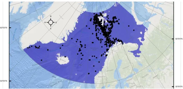
The study area encompasses the Nordic Seas with a spatial extent from N60° to N81° and W45° to E55°, covering main parts of the Greenland-, Norwegian- and the Barents Sea (Fig. 1). The Baltic Sea was left out of the analysis, as fin whales are not native to these waters and the ecosystem differs significantly from the rest of the study area (see Fig. 3). The study area was mainly determined by inspecting fin whale distributional data available (see below), with a buffering area around available sightings. Models were calibrated at an equal-area projection, as if covariate grids were unprojected, a region covering a larger range in latitude of e.g. > 200 km, would have grid cells of varying areas (Elith et al. 2011). This happens especially away from the equator and must be avoided as MaxEnt implicitly assumes equal area cells, when randomly sampling cells (Elith et al. 2011). Optimum projection for the study area was determined using the project wizard tool (Savric et al. 2016)⁴: Polar Lambert azimuthal equal-area projection WGS 1984: EPSG 8326 with a central meridian of 005º 00' E. I used a grid cell size of 100 km² (10 x 10 km) to run the models due the large size of the study area. Further, this resolution seems to be suitable for the high mobility of the species. Land area and the Baltic Sea were masked out from study area, yielding a total of 51595 cells (area in blue in Fig. 3). All species occurrences and EVs were identically projected.

Fig. 3: The study area, covering N60° - N81° and W45° - E55°, including Svalbard and Iceland

4 http://projectionwizard.org

(23)

2.2. Data and Sampling Design

Opportunistic sightings were collected from available data sources: RV Polarstern cruises⁵ (unpublished), GBIF (Global Biodiversity Information Facility)⁶ and iOBIS (Ocean Biogeographic Information System)⁷. Only occurrences between 2004 and 2018 and from an extended definition of summer (May to September) were selected, as summer is the main feeding season of fin whales in the region. Yearly time span was determined according to availability of the Polarstern sighting data. Polarstern data were collected from 27 multidisciplinary research cruises to the Arctic from 2007 to 2018, but with an intermission in data acquisition between 2009 and 2011. Identification of cetaceans was conducted by several nautical officers, and sightings with date and group size were recorded systematically and electronically using ‘WALOG software’ developed by AWI (WALOG vers. 1.3) (Burkhardt 2009). Species were identified to the lowest taxonomic level possible (ranging from species level to “unidentified whale”), associated with a certainty level of identification. Occurrence position was recorded as the position of the vessel at the time of observation. Sightings are considered opportunistic, as no dedicated sighting effort was taken, and no dedicated survey design was implemented. The GBIF data were downloaded from the GBIF website at the desired time span (months/years) and study area extent. Similarly, the iOBIS data were downloaded using robis R-package (Provoost and Bosch 2019). Before running models, sighting data were plotted and occurrences outside of the study area or erroneous (e.g. on land) were removed. After thorough quality control, a total of 1,229 unique sightings remained.

2.3. Environmental Variables

Potential environmental variables were determined based on their ecological relevance for fin whales and their availability (Woodley and Gaskin 1996, Panigada et al. 2008, Druon et al. 2012, Duengen et al. 2018). Initial dynamic variables encompass chlorophyll-a concentration (mean and standard deviation ‘sd’), temperature and salinity at surface and 100 m depth (mean and sd), sea ice concentration (mean and sd), and velocity & sea surface height (mean and sd). Mean and sd represents per grid cell statistically calculated values for the period from 2004 to 2018 and from May to September, when possible (see Table 2 for details).

5 https://www.pangaea.de/expeditions/cr.php/Polarstern

6 www.gbif.org; access date: 01/30/2019

7 https://obis.org; access date: 07/09/2019

(24)

Static environmental variables include bathymetry, slope, aspect and distance to shore, sea ice edge and isobaths (100 m, 200 m and 500 m). In total, 24 environmental layers were prepared at a consistent projection, extent and resolution to be ready to be used by MaxEnt, using ArcGIS (ArcMap 10.6.1, ESRI), QGIS (Version 3.4.5, QGIS Development Team) and R (R Development Core Team 2008). Environmental layers were projected into an equal area projection of Polar Lambert azimuthal equal-area proj.4 of WGS 1984: EPSG 8326 with a central meridian of 005º 00' E (Budic et al. 2015), using spTransform function of raster R-package (Hijmans 2019). For dynamic EVs, standard deviation and climatological mean were calculated for five months (May to September) over the respective (available) amount of years. While for sea ice concentration there was a data gap between May and June 2012, averaged sea ice data for 2012 was based upon July to September data only. Values of grid cells with missing environmental data were interpolated using “Kriging” tool in ArcGIS. Layers were first transformed into points “Raster to Points”, then kriging was implemented with a search radius range between 60,000 and 400,000 m, using a minimum of eight points. Distance to isobaths and shore were calculated using the “Contour” and

“Near” tools in ArcGIS, based on bathymetry. In the settings, the default method “planar” was selected. For the distance to sea ice edge, the ice edge was determined as the major polygon that encompass grid cells with >15% sea ice concentration (Meier and Stroeve 2008 and references therein, Spreen et al. 2008). Values for grid cells intersected with the ice edge line were assigned 0, while grid cells with sea ice concentration < 15% (outside the ice edge) were assigned positive values and grid cells with sea ice concentration > 15% (inside the ice edge) were assigned negative values (Williams et al. 2014). Some grid cells close to land had conspicuous sea ice concentration values, which is termed “land-spillover” or “land contamination of water pixels” (Dr Marcus Huntemann, personal communication, Markus and Cavalieri 2009). To avoid the influence of spurious value of sea ice close to land, a buffer of two grid cells was applied and values at these grid cells were re-estimated using Kriging. Many of the static variables were obtained from the general bathymetric chart of the oceans (GEBCO)⁸, which provides publicly available bathymetry data of the world’s oceans. Temperature and salinity data were obtained by the world ocean atlas (WOA) A5B7⁷ dataset (Boyer et al. 2018). A5B7 refers to the time span 2005 – 2017 and includes a global coverage of Argo floats from 2005. Chlorophyll-a data were obtained from Ocean Color CCI⁵(Sathyendranath et al. 2018).

8 https://www.gebco.net/

(25)

Table 2: Covariates, source and time frame of raw data, * indicates temporal resolution, ** spatial resolution

Covariate Unit Statistic Time

Frame

Resolution Source

Aspect ° 30-arc-sec^** GEBCO⁸

Bathymetry M 30-arc-sec^** GEBCO⁸

Chlorophyll a mg / m³ sd 2004 – 2018 8-day composite^*

OCCI⁹

Distance to SIE Km 2004 – 2018 6.25 km^** AMSR2¹⁰ calculation

Distance to Shore Km 30-arc-sec^** GEBCO⁸

Distance to Isobath 500 Km 30-arc-sec^** GEBCO⁸

Salinity (0, 100 m) unitless mean, sd 2005 – 2017 0.25 x 0.25°^** WOA A5B7¹² Sea Ice Concentration % mean 2004 – 2018 6.25 km^** AMSR2

Sea Surface Height M sd 2004 – 2018 0.25 x 0.25°^** COPERNICUS¹¹

Slope ° 30-arc-sec^** GEBCO⁸

Temperature (0, 100 m) °C sd 2005 – 2017 0.25 x 0.25°^** WOA A5B7¹² Velocity m/s mean 2004 – 2018 0.25 x 0.25°^** COPERNICUS⁶,

calculation

Box-Cox Transformations

To maximize uniformity and obtain normal distribution of variables, potential variable transformations were checked using box-cox transformations (Box and Cox 1964), following Dormann and Kaschner (2010). Accepted transformations that have improved the distribution of variables were distance to 500 m isobath, sea surface salinity (sd), sea surface height (sd), temperature at 100 m depth (sd) and velocity (mean) (Table 3). Transformations of other variables did not improve their distribution and were therefore not implemented.

9 https://esa-oceancolour-cci.org/

10 https://seaice.uni-bremen.de/

11 http://marine.copernicus.eu/services-portfolio/access-to-

products/?option=com_csw&view=details&product_id=SEALEVEL_GLO_PHY_L4_REP_OBSERVATIONS_008_047

12 https://www.nodc.noaa.gov/OC5/indprod.html

(26)

Tests for Multicollinearity

Multicollinearity, the strong correlation between two or more predictor variables, can cause instability in parameter estimation and affect model predictions (Graham 2003, Dormann et al.

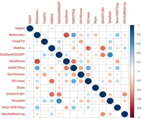
2013), then the least correlated variables should only be used. Only candidate variables with a variance inflation factor (VIF) of <4 were included in the analysis to avoid collinearity, following Zuur et al. (2009). This led to the rejection of nine out of 24 variables. Further, the correlation coefficient between the filtered variables (with VIF <4) was calculated to examine other potential correlation problems. One variable (distance to 200 m isobath) was found to cause correlation issues (correlation coefficient > 0.7) and hence was removed from the analysis. Three environmental variables (mean temperature at 0 and 100 m depth and sd of sea ice concentration) were, based on literature research, expected to be of ecological importance to the species, and were consequently forced in after the removal of highly correlating variables. Since these three candidate variables were still causing collinearity problems, they were excluding from the analysis. In total, nine variables were excluded due to multicollinearity, which resulted in 14 variables to be used in the model (Table 2 and 3, Fig. 4).

Table 3: Overview of transformations and VIF of final EVs used in the model, sd = standard deviation, m = mean

Variable Abbreviation Transformation VIF

Aspect Aspect 1.06

Bathymetry Bathy 3.27

Chlorophyll a sd ChlaSTD 1.38

Distance to Sea Ice Edge Dist2Ice 2.59

Distance to Isobath 500 Dist2Iso500SQRT square root 3.53

Distance to Shore Dist2Shore 2.82

Salinity 0 sd Sal0STDlog log 2.63

Salinity 100 m Sal100mean 2.18

SIC m SICmean 2.64

Slope Slope 1.17

SSH sd SSHSTD1BY inverse 3.28

Temp 0 sd Temp0std 3.00

Temp 100 sd Temp100STDlog log 1.80

Velocity m VelocityMeanLog log 2.07

(27)

Fig. 4: Correlation plot of all variables. Blue is depicting a positive, red a negative correlation, the intensity of shading and size of the circles is indicating the intensity of correlation.

2.4. Modelling procedure

Models were fit using the software MaxEnt v3.4.1 (Philipps et al. 2006, Dudik 2007) available at http://www.cs.princeton.edu/~schapire/maxent. Two modelling approaches were implemented.

First, without accounting for sampling bias: duplicated occurrences in each grid were allowed (modelduplicates). Second, to correct for sampling bias, duplicated occurrences in each grid were removed before running the model (modelnoduplicates). This represents a special form of spatial thinning (e.g. spThin R package, Aiello-Lammens et al. 2019). In order to identify which combination of feature classes and regularization multiplier (RM) lead to the highest performing model, the function ENMevaluate of the ENMeval R package was used (Muscarella et al. 2014), following recommendations from recent literature; e.g. Merow et al. (2013) and Radosavljevic and Anderson (2014). Combinations of six feature classes and eight values for regularization multipliers (ranging from 0.5 to 4, with an increment of 0.5) were selected, leading to 48 models in total. Maxent’s best model parameters were picked according to testing AUC. Spatial blocks were created using the R-package “blockCV” (Valavi et al. 2018).

(28)

Spatial blocks based on presence and background data, where 0 was assigned to background points and 1 to presence locations. Block size was estimated as the median spatial autocorrelation range of the environmental variables, using “spatialAutoRange” function (see Fig. 2). Blocks were then distributed randomly into 4 cross-validation folds using “spatialBlock” function (iterations = 500).

This function tries to find the best allocation of blocks into cross-validation folds, in a way that balances the number of presence and background locations between folds. The same procedure was run separately for each model.

2.4.1. Duplicates Model (modelduplicates)

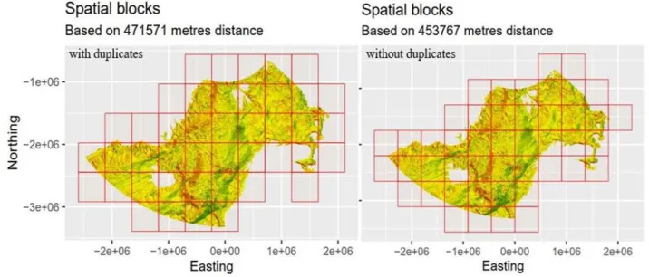
The implemented blockCV mask layer mean range was 471,571 meters (see Fig. 5). This is the specified range by which blocks were created and training/testing data were separated. Data was then manually separated into four spatially cross-validated folds, resulting in four cross-validated models and one full model. For details on model settings see Table 4.

2.4.2. Removed Duplicates Model Arguments (modelnoduplicates)

The implemented blockCV mask layer mean range was 453,767 meters (see Fig. 5). Data were manually separated into four spatially cross-validated folds, resulting in four cross-validated models and one full model. To account for spatial sampling bias, any duplicates within the occurrence data were removed. The removal of duplicates (a duplicate being one or more sightings per grid cell) led to a remainder of 746 occurrences. For details on model settings see Table 4.

Fig. 5: Spatial blocks for model versions with and without duplicates

(29)

Arguments ENMevaluate

Algorithm = maxent.jar Max. iterations = 3000 Method = user

Overlap = true Bin.output = true Parallel = true

Table 4: Overview of the settings for modelduplicates and modelnoduplicates

Settings Duplicate Model Removed Duplicates Model

Add samples to background false false

Maximum Iterations 3000 3000

Jackknife true true

Write background predictions true true

Response curves true true

Pictures true true

Total number of background points 51,595 51,595

Total number of occurrences 1229 746

Afterwards, models were run in R using the maxent function of “dismo” R-package (Hijmans et al.

2017) (for details see the R-script in the appendix). Predictions were made using predict function of the “dismo” package. There are four types of output in MaxEnt: logistic, cumulative, raw and cloglog. Cloglog was chosen as the output form for the analyses, as it is considered to have a stronger theoretical justification than e.g. logistic output (Philipps et al. 2017). All models were stacked and saved. The niche overlap between all models was calculated using calc.niche.overlap function of ENMeval R package (Muscarella et al. 2014).

(30)

The niche overlap metric used was the Schoener’s D (Schoener 1968), which is a statistic for map congruence between pairs of prediction maps, and ranges from 0 (no overlap) to 1 (identical). It was used to identify how much similarity there is between model predictions (Schoener 1968, Warren et al. 2008). Jackknifing and PI were conducted in all model runs, as it enabled the assessment of the relative importance of each of the environmental variables within the respective model.

2.4.3 Visualization of predictions

All prediction maps were prepared using R, describing habitat suitability for each grid cell of the study area, ranging from 0 to 1 (0 being unsuitable, 1 being highly suitable).

3. RESULTS

Ten models with the best combination of MaxEnt’s FC and RM estimated based on spatial-block cross-validation (with keeping and removing duplicated occurrences located at each grid cell:

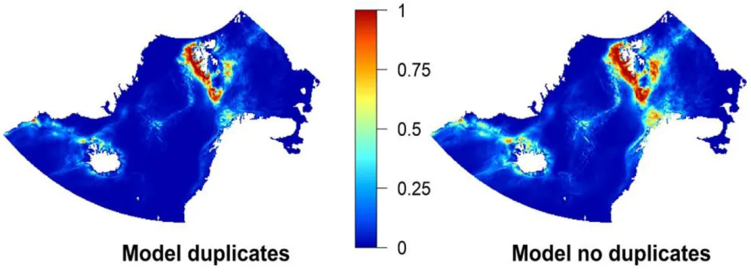
modelduplicates and modelnoduplicates, respectively) were constructed. Two full models and 8 spatially cross-validated models. The two full models of modelduplicates and modelnoduplicates show a similar pattern of habitat suitability, though habitat suitability seems to be rather extensive and not so clustered in the modelnoduplicates (see Fig. 6). Progression of the response curves are similar, though varying in values, while the ratio between variables seems to be somewhat similar (Fig. 13 - 15).

The top important variables of modelduplicates andmodelnoduplicates vary in their composition (see Fig.

9 - 12). In both full models, the seasonal variability (sd) of Chlorophyll-a, sea surface height, variability of temperature at 100 m, aspect, velocity, sea ice concentration, salinity at 100 m, and distance to isobath 500 m were the least contributing variables, with permutation importance less than 6% (see Fig. 11 and Fig. 12). Therefore, their response curves are not discussed further as they are presumed to not have a significant influence on habitat suitability of the fin whale. These variables are only shown in the supplementary (see appendix A).

(31)

3.1 Model with duplicates (modelduplicates)

Five different models were built for the modelduplicates including four cross-validated models built on spatial blocks and one full model. The modelduplicates had an average testing AUC of 0.855 ± 0.016. Habitat suitability is highest along the southwestern coast of Svalbard. Another peak in suitability is on the eastern side of Svalbard, though not as high as on the southwestern coast. This is followed by the north of Norway and on the eastern coast of Greenland up to Iceland (Fig. 6).

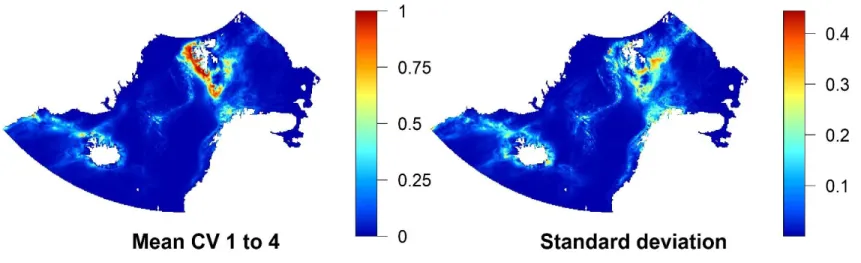
The standard deviation of the predicted distribution of different cross-validation folds of modelduplicates is comparably low. It is highest in the southeast of Svalbard, with patterns similar to general habitat suitability in the prediction map (see Fig. 7).

3.2 Model without duplicates (modelnoduplicates)

Five different models were built for the modelnoduplicates including four cross-validated models built on spatial blocks and one full model. The modelnoduplicates had an average testing AUC of 0.862 ± 0.0098. The pattern of habitat suitability in the modelnoduplicates prediction map is broader and stronger than that of modelduplicates, especially around Svalbard and Norway (Fig. 6). Highest habitat suitability, here too, is along the southwestern coast of Svalbard, though a lot more extensive in the South and southeast of Svalbard. In northern Norway habitat suitability is high as well, higher than in the modelduplicates. Throughout the rest of the study area, patterns do not differ dramatically, though generally habitat suitability seems to be higher in areas of former predicted medium habitat suitability (Fig. 6). Standard deviation is higher than in modelduplicates, mainly in the areas of increased predicted habitat suitability compared to the standard deviation of modelduplicates (Fig. 7 and Fig. 8).

(32)

Fig. 6: Prediction maps of modelduplicates and modelnoduplicates. Habitat suitability ranges from 0 (blue; low) to 1 (red; high).

(33)

Fig. 7: Mean prediction map of the four cross-validated folds of modelduplicates and the according standard deviation. Habitat suitability ranges from 0 (blue; low) to 1 (red; high).

Fig. 8: Mean prediction map of the four cross-validated folds of modelnoduplicates and the according standard deviation. Habitat suitability ranges from 0 (blue; low) to 1 (red; high).