Carl von Ossietzky Universität Oldenburg
Masterstudiengang Biologie
MASTERARBEIT
Studies on the influence of temperature on the feeding rates of important mesograzers in the western Baltic Sea
vorgelegt von Elisa Gülzow
Betreuender Gutachter
Prof. Dr. Pedro Martínez Arbizu Zweiter Gutachter
Prof. Dr. Martin Wahl
Oldenburg, 01. Juni 2015
„In der lebendigen Natur geschieht nichts, was nicht in der Verbindung mit dem Ganzen steht.“
(Johann Wolfgang von Goethe)
I. Table of Content
I. Table of Content ... i
II. List of Figures and tables... ii
III. Zusammenfassung ... iii
IV. Abstract ... iv
1 Introduction ... 1
1.1 Key stone species ... 2
1.2 Mesograzing ... 4
1.3 Temperature - a deciding factor ... 5
1.4 Ambition of the thesis ... 6
2 Material and Methods ... 8
2.1 Setting and preparation ... 8
2.2 Study organisms ... 10
2.3 Experiment ... 11
2.4 Sample processing ... 13
3 Results ... 14
3.1 Idotea spp. ... 17
3.2 Gammarus spp. ... 23
3.3 Result summary ... 29
4 Discussion ... 30
4.1 Result discussion ... 30
4.1.1 Idotea spp. ... 31
4.1.2 Gammarus spp. ... 33
4.1.3 Comparison and summary... 34
4.2 Method discussion ... 35
4.3 Prospects ... 37
V. Appendix ... iv
a. Appendix Idotea spp. ... v
b. Appendix Gammarus spp. ... xiv
VI. Literature ... xix
VII. Acknowledgements ... xxvii
Erklärung ... xxviii
II. List of Figures and tables
Figure 1 Picture of experimental thermo basin ... 8
Figure 2 Map of the Kiel Fjord ... 8
Figure 3 Picture of feed pellet ... 9
Figure 4 Picture of study organism I ... 10
Figure 5 Taxonomic tree of Idotea ... 10
Figure 6 Picture of study organism II ... 10
Figure 7 Taxonomic tree of Gammarus ... 10
Figure 8 Feed pellet after the experiment ... 13
Figure 9 Filtrate of Idotea sp. ... 13
Figure 10 Filter flask and filtration device ... 13
Figure 11 Correlation of faeces and empty squares of Idotea spp. ... 14
Figure 12 Correlation of faeces and empty squares of Gammarus spp. ... 15
Figure 13 Correlation of length and dry weight of Idotea spp. ... 16
Figure 14 Correlation of length and dry weight of Gammarus spp. ... 16
Figure 15 Faeces production Idotea spp. ... 18
Figure 16 Polynomial Fit of faeces production of Idotea spp. ... 19
Figure 17 Empty fly screen squares Idotea spp. ... 20
Figure 18 Quadratic Fit of faeces production of Idotea spp. ... 21
Figure 19 Mortality Idotea spp. ... 22
Figure 20 Faeces production Gammarus spp. ... 24
Figure 21 Rational Function of faeces production of Gammarus spp. ... 25
Figure 22 Empty fly screen squares Gammarus spp. ... 26
Figure 23 Polynomial Fit of empty squares of Gammarus spp. ... 27
Figure 24 Mortality Gammarus spp. ... 28
Table 1 Plan of the temperature adaption period ... 12
Table 2 Formula of curve model for Idotea spp. ... 19
Table 3 Data-fitting curve models of faeces prod. of Idotea spp. ... 19
Table 4 Formula of curve model for Idotea spp. ... 21
Table 5 Data-fitting curve models of empty sq. of Idotea spp. ... 21
Table 6 Formula of curve model for Gammarus spp. ... 25
Table 7 Data-fitting curve models of faeces prod. of Gammarus spp. ... 25
Table 8 Formula of curve model for Gammarus spp. ... 27
Table 9 Data-fitting curve models of empty squares. of Gammarus spp. ... 27
Appendix 1 Recipe for feed pellets ... iv
Appendix 2 Raw data Idotea spp. part 1 ... v
Appendix 3 Raw data Idotea spp. part 2 ... vii
Appendix 4 Faeces production Idotea spp.; output of SPSS ... ix
Appendix 5 T-Test Idotea spp., output of SPSS ... xiii
Appendix 6 Faeces production Idotea spp.; dry weight ... xiii
Appendix 7 Raw data Gammarus spp. part 1 ... xiv
Appendix 8 Raw data of Gammarus spp. part 2 ... xv
III. Zusammenfassung
Der Klimawandel hat zahlreiche Studien hervorgerufen. Viele von ihnen beziehen sich auf Stressökologie. Die Temperatur gilt dabei als entscheidender Einflussfaktor. Es ist bekannt, dass „Keystone species“ in der Lage sind Lebensgemeinschaften und sogar Habitate strukturierend zu prägen.
Mesograzer grasen nicht nur an Algen (top-down), sondern dienen auch als Nahrungsressource für kleinere Fische (bottom-up). Diese Arbeit beschäftigt sich mit dem Einfluss von Temperatur auf die Fraßraten zweier Mesograzer aus der Ostsee, Gammarus spp. und Idotea spp. Es wurde vermutet, dass die Fraßrate in einer Art Optimumskurve auftreten würde. Es wurden Fraßversuche mit Individuen beider Gattungen bei Temperaturen von 5°C bis 30°C durchgeführt.
Als Futter wurden Algen-Pellets verwendet. Es wurde eine Temperaturabhängigkeit der Fraßraten innerhalb beider Gattungen beobachtet.
Die Daten der Individuen von Idotea spp. und Gammarus spp. ergaben in beiden Fällen Optimumskurven. Es wurde eine hohe Mortalität bei höheren Temperaturen als 25°C beobachtet. Die Fraßraten wichtiger Mesograzer könnten in Zukunft zeitweise zunehmen, bis eine Temperatur von etwa 20°C erreicht ist (Optimum) und anschließend aufgrund eines Zusammenbruchs des Stoffwechsels stark abfallen. Wenn Mesograzer aus einem Habitat verschwinden, kann dies schnell drastische Auswirkungen auf die dortige Lebensgemeinschaft haben. Indem wir zu allererst versuchen, einzelne Faktoren auf niederer trophischen Ebene zu verstehen, sind wir möglicherweise besser in der Lage, auch weitergehende und größere Dimensionen der Antworten auf den Klimawandel zu erfassen.
IV. Abstract
Climate change evoked numerous studies. Many of them concentrate on stress ecology. Temperature is considered to be a major factor. Keystone species are known to be able to structure a community or more widely a habitat. Mesograzers not only graze on algae (top-down) but also serve as food supply for smaller fish (bottom-up). We concentrated on the influence of temperature on the feeding rates of two Baltic Sea mesograzers: Gammarus spp. and Idotea spp. It was supposed, that the feeding rates appear in a kind of optimum curve. We conducted feeding experiments with organisms of both genera at temperatures from 5°C to 30°C. As feed, we used algae pellets. There was a temperature dependence in the feeding rate of both genera. The data of the faeces production of Idotea spp. and Gammarus spp. at different temperatures fit to an optimum curve. We observed a high mortality rate at high temperatures in both genera.
The feeding rates of important mesograzers might temporary increase up to a temperature of about 20°C (optimum), but finally will also decrease because of a collapse in the metabolic rate. If grazers remove from a system, the consequences might be drastic changes within the community. By first try to understand single factors at lower trophic levels, we probably might be better able to address the whole dimension of the responses to climate change.
Keywords: Keystone species - Climate Change – Herbivory - Tolerance
1 Introduction
The Baltic Sea is the youngest sea in the Northern Hemisphere, which has its origin approximately 10000 to 15000 years ago after the last glacial. It is the second largest brackish environment and has a maximal depth of 460m and a mean depth of 60m.
The Baltic Sea belongs to the most productive coast ecosystems in the world, but at the same time it belongs to the most threatened ones (Waycott et al., 2009).
As it borders on nine countries, it is widely impacted by influencing factors, such as habitat pollution and overfishing as well as eutrophication and habitat loss (Diaz & Rosenberg, 2008; Eriksson et al., 2009; Halpern et al., 2008).
The Baltic Sea is known for its low salinity with almost freshwater in certain regions. It is influenced and controlled by an exchange with the North Sea and freshwater.
Due to the low salinity, the Baltic Sea is a species-poor ecosystem (Bonsdorff, 2006). Subsequently, to be successful, species might have a broad salinity tolerance. They are often exposed to multiple stressors. These can have singular effects, but can also appear in an additive way (Darling & Cote, 2008; Wernberg et al., 2012). The varying in the oxygen level in the Baltic Sea forces populations to adapt to the changing conditions. That is why they often live at their physiological limit (Feistel et al., 2008). It is known that the populations of the Baltic Sea have a reduced genetic variation than other similar populations in the Atlantic. This might be due to an evolutional selection of extreme genotypes (Johannesson & Andre, 2006). Some species are called “key stone species”, as there is often only one dominant species.
Ecosystems can be influenced by Climate Change (Beaugrand et al., 2010; Pauli et al., 2012) and by consumer populations (Estes et al., 2011; Hughes, 1994;
Paine, 1966; Polis, 1999). Extreme conditions and events are regarded as important driver for the ecosystem structure, as well (Walther et al., 2002).
1.1 Key stone species
A keystone species can be defined as one whose impact on its community or ecosystem is large, and disproportionately large relative to its abundance (Power et al., 1996). Bond (2001) and Mills et al. (1993) defined a keystone species as a species that can exert effects, not only through the commonly known mechanism of consumption, but also through such interactions and processes as competition, mutualism, dispersal, pollination, disease, and by modifying habitats and abiotic factors.
Regarding the above mentioned facts, important key stone species are the isopod Idotea balthica Pallas 1772 (WoRMS, 2015) and the bladder wrack Fucus vesiculosus Linnaeus 1753 (WoRMS, 2015), which will be described later.
Organisms of Idotea spp. are littoral and sublittoral crustaceans living at tidal shores (Naylor, 1955b). They are euryhaline organisms. That means that they are tolerant towards a wide range of salinities. This characteristic enables them to live in the brackish waters of the Baltic Sea (Haage, 1975; Jansson, 1967).
Organisms of Idotea spp. are omnivores, but mainly graze on algae and algal debris, mainly the bladder wrack Fucus vesiculosus (Hemmi & Jormalainen, 2002; Naylor, 1955a, 1955b). In the Baltic Sea, three common species of Idotea can be found. These are I. balthica, I. chelipes Pallas 1766 and I. granulosa Rathke 1843 (WoRMS, 2015). They inhabit Fucus belts and eelgrass communities (Kautsky, 2008). All of these species are very tolerant to varying salinity.
Organisms of Idotea spp. are important primary consumers in littoral communities. They serve as food for several fish (bottom-up) (Haage, 1975, 1976; Hällfors et al., 1975; Jansson, 1967, 1974). They can also have remarkable grazing rates on several algae (top-down) (Leidenberger et al., 2012).
Breeding of Idotea spp. takes place synchronously between May and July. There are two phases of growth. One during the first two months and the other directly before maturity in spring. The largest population size can be found in autumn (Jansson & Matthiesen, 1971; Salemaa, 1979). In winter accumulated algal debris can serve as shelter and rich grazing ground if available, but the organisms often suffer from starvation and mortality (Salemaa, 1978, 1979).
decrease in predation by fish and increased productivity in warmer summers (Haahtela, 1984; Jansson & Matthiesen, 1971; Kangas et al., 1982; Salemaa, 1979, 1986).
Idotea spp. are among the most important herbivores in many systems (Duffy et al., 2001; Jernakoff et al., 1996; Kensley et al., 1995). Within Fucus belts organisms of Idotea balthica are the most important taxon related to their quantity (Korpinen & Jormalainen, 2008). There they constitute about 28% of the crustacean grazers, as well as in eelgrass communities (Bostrom & Bonsdorff, 2000; Schaffelke et al., 1995).
Besides this crucial mesograzers, amphipods build an important part of the communities. One of the amphipods is the genus Gammarus Fabricius 1775 (WoRMS, 2015). In the western Baltic Sea five species of Gammarus occur.
These are G. locusta Fabricius 1775, G. oceanicus Segerstråle, 1947, G.
zaddachi Sexton, 1912, G. salinus Spooner, 1947 and G. d. duebeni Lilljeborg, 1852 (WoRMS, 2015).
Gammarids live in different systems from freshwater to brackish environments like the Baltic Sea. (MacNeil et al., 1997). They live in and under substratum, which serves as shelter but also as food (Fitter & Manuel, 1994). Although gammarids are omnivores, most of the food is provided by algae (Barlöcher &
Kendrick, 1973).The distribution of organisms of Gammarus spp. can be influenced by the oxygen level, acidity and pollution, as well as temperature and salinity (Jeffries & Mills, 1990; Whitehurst & Lindsey, 1990). Due to the fact that gammarids are euryhaline (Bulnheim, 1972), they are able to live in different salinity conditions, so also in the brackish Baltic Sea. They occur from the upper littoral zones to lower subtidal regions and have a broad salinity tolerance (Hartog, 1964; Jazdzeski, 1970; Kinne, 1954; Movaghar, 1964; Segerstrale, 1950).
Organisms of Gammarus spp. often occur together with Idotea spp.
(Leidenberger et al., 2012).
As mentioned above, Fucus vesiculosus is one of the important key stone species in the western Baltic Sea. Most Fucus species occur in habitats, that a more or less stressful like subtidal or the intertidal areas. The distribution zone of Fucus
vesiculosus is also called “Fucus belt”. Compared to the whole Baltic Sea, this area is very species-rich. F. vesiculosus is an important organism as it serves as perennial habitat for many species and builds predictable a basis of the food web (Hawkins & Hartnoll, 1983).
It is already known that F. vesiculosus is able to build up a defence mechanism against biotic stressors. This is thought to be induced by for example grazing (Nietsch, 2009; Pavia et al., 1997; S. Rohde et al., 2004; Toth & Pavia, 2007;
Weinberger et al., 2011). In this way, F. vesiculosus can control the richness of the herbivory community (Van Zandt & Agrawal, 2004).
Although a positive growth up to a depth of 5 to 6m has been observed in summer (Sven Rohde et al., 2008; Wahl et al., 2010), there is a reduction of 95% of the distribution range of F. vesiculosus, as it changed from a depth of 10m in the 1960s to a depth of just 1.5m today (Berger et al., 2004; Vogt & Schramm, 1991).
Possible reasons for this decrease are eutrophication, epibiosis and grazing (Jormalainen & Ramsay, 2009; Krause-Jensen et al., 2009; Sven Rohde et al., 2008). Overfishing and overall climate change might also be factors (Ugarte et al., 2010). F. vesiculosus is thought to be very sensitive to future summer temperatures, which might have a huge impact on communities (Raddatz et al., in prep.). It is possible that high grazing rates by amphipods and isopods like Gammarus spp. and Idotea spp. are also able to reduce Fucus populations at several localities (Engkvist et al., 2000).
Fucus vesiculosus serves as habitat and food supply for the most abundant grazers in the Baltic Sea. These are the amphipod Gammarus spp. and the isopod Idotea spp. (Anders & Moller, 1983).
1.2 Mesograzing
Mesograzers have a structuring and decomposing role within the littoral communities. Amphipods and Isopods effect the biomass and diversity of vegetation (Brawley & Adey, 1981a, 1981c; Lopez et al., 1977; Robertson &
Mann, 1980; Zimmerman et al., 1979). Herbivory is told to belong to the most important biotic factors regarding the development of a community at rocky
Herbivory by isopods, amphipods or gastropods can act in a mild but also in a severe and harmful way. A high density in herbivore populations can cause huge damage to the macroalgae. A positive effect is also possiblr, if they remove harmful epiphytes from algae (Brawley & Adey, 1981c; Nicotri, 1977; Shacklock
& Croft, 1981). Thereby, they can affect stages of Fucus from germlings to adults (Dethier & Williams, 2009; Long et al., 2007; Pennings et al., 2000). There is a seasonal fluctuation of grazing pressure. It is low in winter and early summer when mesograzers are inactive or have low densities (Kotta et al., 2006). In contrast, grazing pressure is high in late summer when the density of juveniles is high (Engkvist et al., 2000; Korpinen et al., 2010).
Not only direct effects of mesograzers like on the biomass have been observed.
They can also mediate influences of climate change in a direct way on lower trophic levels (O'Connor, 2009; O'Connor et al., 2011; Walther, 2004). Alsterberg et al. (2013) found out that mesograzers strongly affect the balance between bottom-up and top-down effects.
1.3 Temperature - a deciding factor
In 1990 (Lüning) a temperature of 20°C was told as highest water temperature, that lasted for longer periods than weeks within the natural distribution range of Fucus vesiculosus. Nowadays, the water temperature is already close to the limit in the upper 5m of the western Baltic Sea between June and August (Wahl, unpubl.). The water temperature is expected to rise for 3° to 5°C in the course of this century (BACC, 2008; IPCC, 2007). Ecosystems are already exposed to extremely high temperatures during summer (Wahl et al., 2010). Due to the low biotic diversity within the brackish Baltic Sea, there is a high risk of disturbance in the littoral communities (Hällfors et al., 1981).
Mesograzing is thought to increase with higher temperatures (BACC, 2008;
IPCC, 2007). During former feeding experiments, Weinberger et al. (2011) detected a higher palatability of algae at 20°C. This might be due to a possible lower ability to induced defence which resulted higher grazing.
For F. vesiculosus, warming is documented to have stress effects from a temperature of 20°C (Pearson et al., 2009; S. Rohde & Wahl, 2008). Besides, in summer 2014, Raddatz et al. (in prep.) observed a drastic decrease within the populations of Gammarus spp. and Idotea spp., while the temperature increased
up to 29°C. There might have been a thermal border and the metabolic rate of algae and grazers might be influenced by temperature (Jenkins et al., 2001).
A lot of marine organisms already live close to their thermal tolerance limit (Hughes et al., 2003; Somero, 2002).
It is expected that a predicted climate change scenario will shift the environmental variables due to temperature, which may impact numerous species and marine coastal systems (Harley et al., 2006; IPCC, 2007; Parmesan, 2006). As suggested by Phillipart et al. (2003) there might be earlier spawning in several species due to warmer conditions, which might end up in a mismatch towards food supply.
Species with broad ecological niches might be able to better tolerate environmental changes. Such as species from the fluctuating Baltic Sea might be more flexible than species from more stable environments (Schneider, 2008). A consequence of a rising temperature in future, might be a shift along with their tolerance towards high temperature, as well as their capability to adapt to new conditions (Fields et al., 1993; Lubchenco et al., 1993).
1.4 Ambition of the thesis
In the last decades, numerous studies concerning climate change and its environmental effects were carried out. Many of them provide an insight into the stress ecology of different habitats. Single stressor and multiple stressor, which act in an additive way, were described. To be able to address the prospective responses of communities to climate change, it is important to do a first step:
Understanding changes at low levels. The predicted 3° to 5°C increase in temperature may seem small, but can have huge impacts as not only direct but indirect effects of warming might be important (Wernberg et al., 2012).
Climate change has to be regarded from the lowest trophic level of communities, genera or even species. It is necessary to understand how organisms cope with changes.
Manipulating single stressors might help to understand and modulate possible scenarios of multiple ones.
temperature dependency of feeding rates of important mesograzers in the western Baltic Sea. Due to the studies of Pearson et al. (2009), Rohde & Wahl (2008) and Raddatz et al. (in prep.), this dependency is supposed to appear in an optimum curve with an optimum around 20°C.
H0: The feeding rate and so the faeces production increases with increasing temperature. There is a linear correlation between them.
H: The feeding rate and so the faeces production appears in a temperature dependent optimum with a quadratic function.
2 Material and Methods
2.1 Setting and preparation
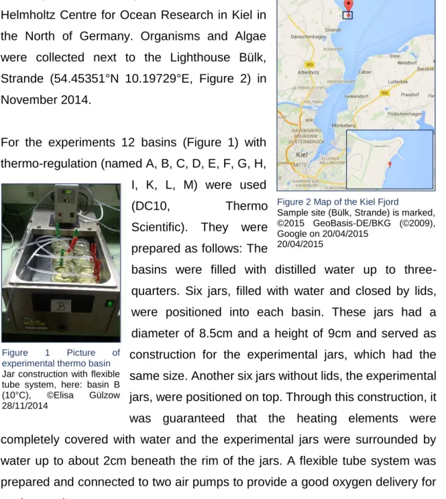
The experiments took place at the GEOMAR Helmholtz Centre for Ocean Research in Kiel in the North of Germany. Organisms and Algae were collected next to the Lighthouse Bülk, Strande (54.45351°N 10.19729°E, Figure 2) in November 2014.
For the experiments 12 basins (Figure 1) with thermo-regulation (named A, B, C, D, E, F, G, H, I, K, L, M) were used
(DC10, Thermo
Scientific). They were prepared as follows: The
basins were filled with distilled water up to three- quarters. Six jars, filled with water and closed by lids, were positioned into each basin. These jars had a diameter of 8.5cm and a height of 9cm and served as construction for the experimental jars, which had the same size. Another six jars without lids, the experimental jars, were positioned on top. Through this construction, it was guaranteed that the heating elements were completely covered with water and the experimental jars were surrounded by water up to about 2cm beneath the rim of the jars. A flexible tube system was prepared and connected to two air pumps to provide a good oxygen delivery for each organism.
For feeding experiments with Idotea balthica, an artificial feed has already been developed at the GEOMAR. Before starting the experiments, the collected thalli of Fucus vesiculosus were freeze-dried and grinded to a fine and homogeneous
Figure 2 Map of the Kiel Fjord
Sample site (Bülk, Strande) is marked,
©2015 GeoBasis-DE/BKG (©2009), Google on 20/04/2015
20/04/2015
Figure 1 Picture of experimental thermo basin Jar construction with flexible tube system, here: basin B (10°C), ©Elisa Gülzow 28/11/2014
Fresh artificial feed was prepared for every new experiment of the organisms of one basin. For this purpose 1g algae powder was mixed with 4ml distilled water and 0,36g agar powder was mixed with 5ml distilled water. Two squares of baking paper (20 x 20cm) and one square of fly screen (5 x 5cm) were prepared.
Additionally, a stable plate of plexiglass was laid out. The agar-water mixture was heated in the microwave at 800 watt until it boiled up. It was stirred at least once. The algae-water mixture was quickly filled into the hot mixture and stirred quickly. The resulting gel was put onto the fly screen and pressed between the two baking paper squares by using the plexiglass plate. After some seconds the gel was solid and had filled the squares of the fly screen. The fly screen could be cut into small squares for the experiment. Feed pellets of approximately 1cm x 1cm,
composed of small screen squares of 11 x 11 squares were used for the experiment (Figure 3 Picture of feed pellet
Algae pellet used in the feeding experiments, ©Elisa Gülzow 12/12/2014).
All of the pictures were taken by Sony Xperia S, 12 MP.
Figure 3 Picture of feed pellet
Algae pellet used in the feeding experiments,
©Elisa Gülzow 12/12/2014
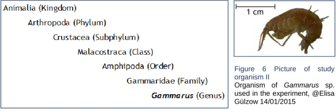
2.2 Study organisms
The collected organisms were organisms of Idotea (Figure 4, Figure 5) and Gammarus (Figure 6 and Figure 7).
The organisms of Gammarus were organisms of Gammarus locusta, Gammarus oceanicus and Gammarus salina. Organisms of Idotea were organisms of Idotea balthica and Idotea granulosa.
Figure 4 Picture of study organism I
Organism of Idotea balthica used in the experiment, @Elisa Gülzow 21/12/2014
Figure 5 Taxonomic tree of Idotea
Classification of the Genus Idotea according to the World Register of Marine Species at http://www.marinespecies.org/aphia.php?p
=taxdetails&id=118454 on 21/04/2015
Figure 7 Taxonomic tree of Gammarus
Classification of the Genus Gammarus according to the World Register of Marine Species at http://www.marinespecies.org/aphia.php?p
=taxdetails&id=101537 on 21/04/2015
Figure 6 Picture of study organism II
Organism of Gammarus sp.
used in the experiment, @Elisa Gülzow 14/01/2015
2.3 Experiment
The entire feeding experiment took about three weeks. During this period, the organisms were inserted into experimental jars. Temperature was increased or decreased to the respective end temperature. Prior to the feeding experiments, the organisms had one week of acclimatization.
Detailed description: 72 experimental jars were prepared. They were filled with salt water from the GEOMAR system in the main building. The water came from the Baltic Sea and had already been sand-filtered by the system of the GEOMAR.
Start temperature of the water in all basins was 12°C, which was the temperature of the Baltic Sea, when the experiment started. Thalli of Fucus vesiculosus were prepared and put into the jars. These had several branches to serve as feed and to give hold to the organisms. The length of each organism was measured by using a geometry set square and noted for later calculations and to get a reference value. The organisms were randomly put into the experiment jars, whereby there was only one organism in each jar. After that, the ends of the prepared air system were transferred into the experimental jars and fixed by a clothes peg, so that the air bubbles were not too strong and not too weak.
The temperature was changed twice a day towards the end temperature of the respective basin (Table 1). As described above, every basin started at a temperature of 12°C. The end temperatures were 5°C, 10°C, 15°C, 20°C, 24°C, 25°C, 26°C, 27°C, 28°C, 29°C and 30°C. There was also one basin where the temperature was kept at 12°C to control the influence of the experimental design.
Once the end temperature in a basin has been reached, it was kept for seven days in order to allow for the organisms to acclimate prior the start of the experiment. After these seven days three steps of the feeding experiment were carried out. In the first step, the Fucus thalli of the respective jars were removed to make sure that the organisms were all hungry during the experiment and the results were not influenced by any other feed than the artificial.
Table 1 Plan of the temperature adaption period
Daily steps of the temperature adaption in °C, one-week-acclimatization, feeding experiment (red=no Fucus thalli, green=feed pellet added, purple=feed pellet removed + end of experiment)
After this starvation-phase of 24 hours, the second step was to remove the faeces of the former day and to insert a feed pellet into each jar for the next 24 hours. In the third step, the feed pellets were removed and the faeces were taken out of the jars.
During the temperature adaption, water was changed every second to third day by removing up to 50% of the ‘old’ water and replacing it by fresh water from the system. This fresh water had been stored in the respective basin and hence already had the right temperature. To exclude manipulation through a modified salinity due to evaporation, the water level was marked at the beginning and checked several times a day. A minor deviation from this level was compensated by adding some drops of distilled water. The Fucus thalli were replaced by fresh thalli every few days to make sure that the organisms have fresh feed during the adaption. Organisms of Gammarus were more active and swam around during the adaption time. Therefore, an additional piece of empty fly screen was inserted during the feeding experiment to give them a little more hold so that they were not twirled around by bubbles of the air system.
Date
A B C D E F G H I K L M
26.11. 12 12 12 12 12 12 12 12 12 12 12 12
27.11. 10 10 12 14 14 14 14 14 14 14 14 14
28.11. 8 10 12 15 16 16 16 16 16 16 16 16
29.11. 6 10 12 15 18 18 18 18 18 18 18 18
30.11. 5 10 12 15 20 20 20 20 20 20 20 20
1.12. 5 10 12 15 20 22 22 22 22 22 22 22
2.12. 5 10 12 15 20 24 24 24 24 24 24 24
3.12. 5 10 12 15 20 24 25 26 26 26 26 26
4.12. 5 10 12 15 20 24 25 26 27 28 28 28
5.12. 5 10 12 15 20 24 25 26 27 28 29 30
6.12. 5 10 12 15 20 24 25 26 27 28 29 30
7.12. 5 12 15 20 24 25 26 27 28 29 30
8.12. 5 20 24 25 26 27 28 29 30
9.12. 5 20 24 25 26 27 28 29 30
10.12. 24 25 26 27 28 29 30
11.12. 24 25 26 27 28 29 30
12.12. 25 26 27 28 29 30
13.12. 27 28 29 30
14.12. 29 30
Basin
2.4 Sample processing
After the feeding experiment of 24 hours, the feed pellet was removed and the faeces of these 24 hours were collected by a syringe. The feed pellet and the collected faeces of each organism were stored separately to be able to assign the probes to the respective organism.
The feed pellets were checked for empty squares (Figure 8). Squares were counted as an empty squares, when more than half of the square was eaten. The total numbers of eaten squares was noticed for each organism.
The organisms were put into the freezer for 20 minutes at -18°C to sedate them and were subsequently dried in a heating cabinet for 24 hours at 80°C.
Afterwards, the organisms were weighed to determine their dry weight to get a reference value for the amount of faeces and eaten squares.
The faeces were filtered through glass microfiber filters with a pore size of 1.2µm (GF/C 25mm, Whatman) (Figure 9). The dry weight of these filters was already defined before filtration. A diaphragm vacuum pump (KNF), a filtration device and a filter flask (both Duran) were used for the filtration (Figure 10). The faeces-including filters
were dried in the heating cabinet for 24 hours at 80°C. Finally the dry weights were determined by weighing the dried faeces-including filters. By subtracting the dry weight of the respective filters the exact dry weight of the faeces of each organism could be analysed.
For the analyses and representation IBM SPSS statistics 22, CurveExpert Version 1.40 and Microsoft Excel 2013 were used.
Figure 8 Feed pellet after the experiment
Empty squares can be seen, which have been eaten by a study organisms during the feeding experiment,
@Elisa Gülzow
28/11/2014
Figure 9 Filtrate of Idotea sp.
Filtered faeces of a study organism before drying,
@Elisa Gülzow 28/11/2014
Figure 10 Filter flask and filtration device Filtration equipment for the progression of the collected faeces probes, @Elisa Gülzow 28/11/2014
3 Results
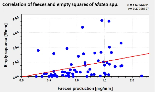
There were two possible indicators for the feeding rates of Idotea spp. and Gammarus spp., the production of faeces and the empty fly screen squares of the feed pellets. Figure 11 and Figure 12 show correlations between the faeces production and empty fly screen squares, both standardised by the length of the organisms. There was a linear correlation with a coefficient of r=0.37 for the data of the organisms of Idotea spp. (Figure 11). A coefficient of r=0.59 could be found for a linear correlation between data of Gammarus spp. (Figure 12).
Figure 11 Correlation of faeces and empty squares of Idotea spp.
Correlation between quantity of faeces production and empty fly screen squares for the organisms of Idotea spp. Correlation coefficient r=0.37 and standard error S=1.68.
Figure 12 Correlation of faeces and empty squares of Gammarus spp.
Correlation between quantity of faeces production and empty fly screen squares for the organisms of Gammarus spp. Correlation coefficient r=0.59 and standard error S=1.75.
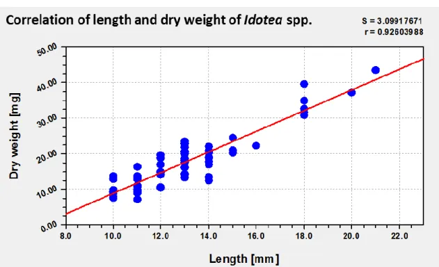
To compare the length and the dry weight of the organisms as standardizations for the resulting data, two kinds of correlations were made. These should help to decide about the best kind of standardization. The first correlation was done between the length and the dry weight of the organisms of Idotea spp. The same was done for Gammarus spp. A linear correlation with a coefficient of r=0.93 between the length [mm] and the dry weight [mg] of Idotea spp. (Figure 13.) and a coefficient of r=0.94 for Gammarus spp. (Figure 14 Correlation of length and dry weight of Gammarus spp.) could be determined.
Figure 13 Correlation of length and dry weight of Idotea spp.
Length and dry weight of each organism of Idotea spp. with a linear regression. Standard error (S)=3.1 and correlation coefficient (r)=0.93.
Figure 14 Correlation of length and dry weight of Gammarus spp.
Length and dry weight of each organism of Gammarus spp. with a linear regression. Standard error S=5.54 and correlation coefficient r=0.94.
3.1 Idotea spp.
The quantity of faeces production in dependence of temperature was tested on organisms of the genus Idotea. The resulting data were standardised by the length of the respective organisms. Therefore, results are presented in the quantity of faeces [mg] per millimetre of the organisms.
The control basin (C) with a temperature of 12°C was used to determine if the experimental design had an influence on the resulting data. The feeding experiment was conducted at the beginning and the end of the time and the faeces production was analysed. A t-test showed that these data were significantly not different (p=0.735). No mortality was observed in this basin.
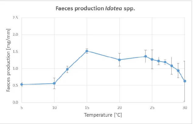
The quantities of faeces production at different temperatures are indicated in Figure 15. A low faeces production was observed at 5°C and increased to the maximum of faeces production at 15°C. The quantity of faeces decreased continuously until 30°C. It could be established that the amount of faeces was similar at 5°C and at 30°C. For the analysis, a variance homogeneity test was carried out, which showed that the data were not homogenous (p=0.000). The equality of the mean values was tested by a Welch-test which was significant (p=0.000). Consequently, the data were not equal. As a post-hoc test the Scheffé- test was used to compare the mean values of the data. A significant difference between 5°C and 15°C (p=0.041) could be established. There was a significant lower faeces production at 5°C than at 15°C. No significant differences within the higher temperature steps were identified.
Figure 15 Faeces production Idotea spp.
Mean faeces production per experimental basin at different temperatures. Standardised by length of organisms. Significant difference (p=0.041) between 5°C and 15°C.
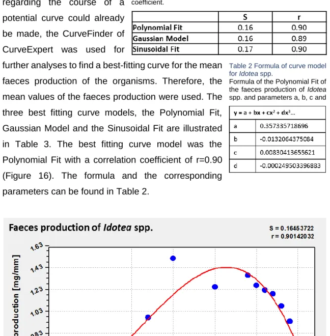
As an educated guess regarding the course of a potential curve could already be made, the CurveFinder of CurveExpert was used for
further analyses to find a best-fitting curve for the mean faeces production of the organisms. Therefore, the mean values of the faeces production were used. The three best fitting curve models, the Polynomial Fit, Gaussian Model and the Sinusoidal Fit are illustrated in Table 3. The best fitting curve model was the Polynomial Fit with a correlation coefficient of r=0.90 (Figure 16). The formula and the corresponding parameters can be found in Table 2.
Table 3 Data-fitting curve models of faeces prod. of Idotea spp.
Three best fitting curve models. S= standard error; r= correlation coefficient.
Figure 16 Polynomial Fit of faeces production of Idotea spp.
Faeces production of Idotea spp. at different temperatures. Best fitting curve model for resulting data. S=
standard error; r= correlation coefficient.
Table 2 Formula of curve model for Idotea spp.
Formula of the Polynomial Fit of the faeces production of Idotea spp. and parameters a, b, c and d
In addition to the quantity of faeces production, the empty fly screen squares of the feed pellets of the corresponding organisms from different temperatures were inspected. These data were also standardised by the length of the organisms.
The results are consequently presented in the quantity of empty squares per millimetre of the organism. Figure 17 shows the results of the mean values of empty fly screen squares at different temperatures. The quantity of empty squares increased to a peak at 15°C while there were less empty squares at 20°C. The next peak was at 25°C. There was a decrease in the quantity of empty squares until a temperature of 30°C was reached. To analyse these data, a variance homogeneity test released that the data were homogenous (p=0.004).
The following ANOVA was not significant (p=0.209). There was no significant difference between the mean values of these data.
Figure 17 Empty fly screen squares Idotea spp.
Mean numbers of empty fly screen squares per experimental basin at different temperatures. Standardised by length of organisms.
For the data of the empty squares, a best-fitting curve model was searched, as well, by using the CurveFinder of CurveExpert. Table 5 shows
the three best-fitting curve models for the data. As a Sinusoidal Fit is not appropriate for this kind of data set, Table 4 shows the formula of the quadratic curve model and its parameters. The Quadratic Fit had a correlation coefficient of r=0.65.
The Quadratic Fit of the empty squares is illustrated in Figure 18 Quadratic Fit of faeces production of Idotea spp..
Figure 18 Quadratic Fit of faeces production of Idotea spp.
Empty squares of Idotea spp. at different temperatures. Best fitting curve model for resulting data. S=
standard error; r= correlation coefficient.
Table 5 Data-fitting curve models of empty sq. of Idotea spp.
Three best fitting curve models. S= standard error; r= correlation coefficient.
Table 4 Formula of curve model for Idotea spp.
Formula of the Quadratic Fit of the empty squares of Idotea spp. and parameters a, b, c and
As side effect, the mortality was considered for organisms of Idotea spp. during the whole experiment. The results are presented in the percentage of mortality in the respective basins and illustrated in Figure 19. There was no mortality in the basins which reached a final temperature of 5°C to 20°C or 25°C and 26°C while a third of the organisms of basin F that reached a temperature of 24°C, died. A high mortality was also observed at higher temperatures. Half of the organisms of basin K (28°C) and a third of the organisms of basin L (29°C). There was a mortality rate of 15% in the basins I (27°C) and M (30°C).
Figure 19 Mortality Idotea spp.
Percentage mortality per experimental basin. Six organisms in each basin.
3.2 Gammarus spp.
For the organisms of the genus Gammarus the quantity of faeces production was tested at different temperatures. These results were standardised by the length of the particular organisms, so that the results are presented in the mean quantity of faeces production [mg] per millimetre of organism.
A control basin (C) with a temperature of 12°C for Gammarus spp. was used in order to prove that the experimental design had no effect on the quantity of faeces production. The feeding experiment was carried out at the beginning and the end of the time. A t-test was used to analyse the faeces production of both experimental parts. It showed that these data were significantly not different (p=0.359). One of five organisms of this basin died during the keeping.
The results of the feeding experiments at the different temperatures are shown in Figure 20. There was an increase of faeces production from 5°C upwards, which had a peak at 20°C. A decrease of the production of faeces could be observed in the following basins: In the 27°C-basin (I), the faeces production was low like at the beginning 5°C. Due to mortality, there were no data for basins K, L and M.
Data were analysed by a variance homogeneity test that showed that the data were homogenous (p=0.955). An ANOVA was not significant (p=0.166). There were no significant differences between the mean values of these Gammarus data.
Figure 20 Faeces production Gammarus spp.
Mean faeces production per experimental basin at different temperatures. Standardised by length of organisms.
By using the CurveFinder of CurveExpert, the best fitting curve model for the data could be found. Here the data of every single organisms was used. The three best fitting
models can be seen in Table 7 Data-fitting curve models of faeces prod. of Gammarus spp.. These were a Rational Function, Polynomial Fit and a Reciprocal Quadratic Function. The best fitting curve model was a Rational Function with a correlation coefficient of r=0.95. This curve is illustrated in Figure 21 Rational Function of faeces production of Gammarus spp.. The corresponding formula and its parameters can be found in Table 6.
Figure 21 Rational Function of faeces production of Gammarus spp.
Faeces production of Gammarus spp. at different temperatures. Best fitting curve model for resulting data.
S= standard error; r= correlation coefficient.
Table 7 Data-fitting curve models of faeces prod. of Gammarus spp.
Three best fitting curve models. S= standard error; r= correlation coefficient.
Table 6 Formula of curve model for Gammarus spp.
Formula of the Rational Function of the faeces production of Gammarus spp.
and parameters a, b, c and d
For the organisms of Gammarus, the number of empty fly screen squares of the feed pellets was also quantified. The results were standardised by the length of the organisms. Collected data can be seen in Figure 22. The feed pellets of basin A (5°C) showed a very low quantity of empty squares. There was a continuous increase up to a peak in the basin with 20°C. The next small peak could be observed at 25°C. There were no empty or little empty squares in the pellets of the basins with a final temperature of 24°C and 27°C. No results can be given for the basins with temperatures of 28°C to 30°C due to mortality. A variance homogeneity test showed that the data were homogenous (p=0.028). A following ANOVA was not significant (p=0.596). There was no significant difference between the mean values of the empty squares.
Figure 22 Empty fly screen squares Gammarus spp.
Mean numbers of empty fly screen squares per experimental basin at different temperatures. Standardised by length of organisms.
The CurveFinder of CurveExpert was again used for these data. A best-fitting curve model was searched for the data of the empty fly screen squares of the
experiments of organisms of Gammarus spp. Table 9 Data-fitting curve models of empty squares. of Gammarus spp.shows the three best-fitting curve model for our data. As the Sinusoidal Fit is not appropriate to the data, the Polynomial Fit is illustrated in Figure 23. This curve had a correlation coefficient of r=0.82. Table 8 shows the formula of this curve and the respective parameters.
Figure 23 Polynomial Fit of empty squares of Gammarus spp.
Empty fly screen squares of Gammarus spp. at different temperatures. Best fitting curve model for resulting data. S= standard error; r= correlation coefficient.
Table 9 Data-fitting curve models of empty squares. of Gammarus spp.
Three best fitting curve models. S= standard error; r= correlation coefficient.
Table 8 Formula of curve model for Gammarus spp.
Formula of the Rational Function of the empty squares of Gammarus spp
A side effect of the experiments of Gammarus spp. was also the mortality. This factor was monitored and noticed during the whole experiment. Figure 24 shows the percentage of dead organisms in the respective basins. As basins A to D started with 5 organisms, the percentages of these basins refer to a 100%-rate of five organisms instead of six. This was due to the quantity of organisms. A low mortality of 20% could be established in the lower tempered basins. No mortality was monitored in the basins, which reached 15°C and 20°C. The 24°C-basin showed a high mortality of two-thirds. In the basin that reached 25°C, a low mortality of less than 20% was realized. High mortality rates could be detected at higher temperatures. Basins H (26°C) and I (27°C) had a mortality of more than 80%. In the basins with temperatures between 28°C to 30°C, all of the organisms of Gammarus died.
Figure 24 Mortality Gammarus spp.
Percentage mortality per experimental basin. A-D with 100%-rate of five organisms, other basins with six organisms.
3.3 Result summary
No significant results could be found by using the quantity of fly screen squares as indicator for the feeding rates of organisms of Idotea and Gammarus. During the experiments of the organisms of Idotea spp., a significant higher mean faeces production could be established at a temperature of 15°C than at a low temperature of 5°C. During the experiments of the organisms of Gammarus spp., no significant results could be found regarding the quantity of faeces production.
In both genera, mortality was higher in basins that reached higher temperatures of more than 25°C than in basins that had a lower final temperature. Especially, organisms of Gammarus spp. died when higher temperatures were reached. The data of the faeces production of Idotea spp. at different temperatures fit to a polynomial curve model. The data of the faeces production of organisms of Gammarus spp. fit to a rational curve model. The experimental time had no effect on the results.
4 Discussion
4.1 Result discussion
Prior to analysing the resulting data of the feeding experiments, the task was to find out the possible indicator suitable for the analyses. There was the possibility to indicate the feeding rates of the organisms of Idotea spp. and Gammarus spp.
by quantifying the empty fly screen squares of the feed pellets. A second possible indicator for the feeding rates was to quantify the faeces production. A correlation was done between the faeces production and the empty fly screen squares of the experiments of both genera. In both cases, neither for Idotea spp. nor for Gammarus spp., there was a very good linear correlation between the data sets.
The method of quantifying the empty fly screen squares seemed to be very imprecise. This will be explained more detailed in the method discussion.
Therefore, the faeces production was more suitable for the analyses.
A second task was to find out the best way for a standardization of the data. The reason for it was, that the organisms were not of the same size, so that for a comparison there had to be a kind of standardization. A correlation of the length and the dry weight of the organisms of Idotea spp. and Gammarus spp. was done.
There was a good linear correlation between the data sets. It could be assumed that both, the length and the dry weight, could be used as standardisation value.
This was tested during a third correlation between the faeces production standardised with the length and the faeces production standardised with the dry weight. We also found a good linear correlation for the correlations of organisms of Idotea spp. and Gammarus spp. Obviously both could be used as standardisation value. Here, the length was used to standardise the data.
4.1.1 Idotea spp.
The faeces production of organisms of Idotea spp. in dependence of temperature was investigated as an indicator for the feeding rate.
When we compared the mean values of the faeces production of the different tempered basins, we detected a significant difference in the mean values belonging to 5°C and 15°C. Subsequently, it can be supposed, that there is indeed a higher feeding rate at 15°C than at 5°C. As explained above, the resulting data of the quantification of empty fly screen squares seemed to be imprecise and were influenced by the feeding behaviour of the organisms as they often only ate at the surface of the feed pellets. These data were not appropriate to be used as indicator for the feeding rate.
The assumption was that there could be a kind of optimum curve for the feeding rates of organisms of Idotea spp. A polynomial curve model was found as best- fitting model for these data. While this curve model had a correlation coefficient of r=0.90, the previous assumption could be largely confirmed. It was supposed that there would be a low metabolic rate at low temperatures which might be followed by a low feeding rate. An increase was assumed up to a temperature of approximately 20°C with a subsequent more abrupt decrease. The curve model of the faeces production of Idotea spp. showed exactly the course that was expected. The curve showed a slow increase of the faeces production, an optimum at the beginning of 20°C and a decrease of the faeces production up to 30°C.
Observations during the experiment showed a clear difference in the vitality of organisms at temperatures of 5°C and 21°C. The organisms in the 5°C-basin moved very slowly and seemed lethargic. The organisms in the basin that reached 21°C were very active and swam around a lot. These observations suited to the resulting data. The low vitality at lower temperatures could be explained by a low metabolic rate which takes fewer energy and makes it possible to calm down the feeding rates.
As assumed, the metabolic rate seemed to increase to a kind of optimum, which was followed by a higher vitality and a higher feeding rate. A sudden decrease in
the feeding rates could be established, when the temperature exceeded this optimum. A lower vitality could be observed at this temperatures. This could be due to a decrease in the metabolic rate because of heating stress.
The mortality rates of the organisms of Idotea spp. showed a higher mortality at the upper temperatures than the lower ones. It seemed as if lower temperatures could be tolerated more easily. The higher temperatures above the middle 20°C were often followed by a high mortality rate. This matched the former assumptions that higher temperatures could constitute a problem for the surival of the organisms.
The high mortality in basin F (24°C) was proved by looking for any technical influences like light or a false temperature on the display of the experimental basin. No indication for the high mortality could be found. This temperature might be a critical point for the organisms. The organisms of basin F might also have been more sensitive than the others.
4.1.2 Gammarus spp.
For the organisms of Gammarus spp., the faeces production was also quantified in dependence of the temperature as an indicator for the feeding rate.
During a comparison of the mean values of the faeces production from organisms of Gammarus spp., no significant differences could be found. The quantification of the empty fly screen squares were, as well, rather imprecise as the organisms of Gammarus spp. often only ate at the surface of the feed pellet, but more often just ate from the margin of the pellet. Therefore, these results should be considered with caution. The faeces production might have given better resulting data about the feeding rates of the organisms of Gammarus spp. No statement can be made for the organisms in the basins that reached temperatures of 28°C and above. There was a mortality rate of 100%.
It was guessed that data could appear in a kind of optimum curve for the faeces production of Gammarus spp., as well. A Rational Function was considered to be the best-fitting curve for the data with a correlation coefficient of r=0.95. It was expected, that there would be an increase of the feeding rate with an optimum around 20°C and a more or less sudden decrease. The rational curve showed these course of the results. The optimum was situated slightly below 20°C. There was indeed a slower increase and a sudden decrease of the faeces production.
During the experiments, the mortality of the organisms of Gammarus spp has also been observed. Mortality could be established in every basin except basin D and E that reached 15°C and 20°C. It can be assumed, that organisms of Gammarus spp. are very intolerant to temperatures above 20°C. In that basins up to 100% of the organisms died. In basins A to C, only one organism died.
Thus, these temperatures might not create such huge problems like higher ones.
During the experiments of the organisms of Idotea spp. a higher mortality in basin F, which reached 24°C, was detected. This basin was inspected for any other influences but no external reason for the high mortality rate could be found.
Therefore, it could be supposed, that there might be a critical point for the metabolic rate and surviving of the organisms. Another reason could be, that this was just coincidental.
4.1.3 Comparison and summary
The course of the faeces production over the different temperature steps were very similar between both genera. Both showed a slow increase and a more or less sudden decrease in the production of faeces. Both genera seemed to better tolerate low temperatures than high temperatures. The organisms of Gammarus spp. seemed to be more mortality-prone than the organisms of Idotea spp. The best-fitting curve model showed an optimum above 20°C for Idotea spp. and an optimum below 20°C for Gammarus spp. This might be an indicator for a lower tolerance limit of Gammarus spp. towards temperature.
Mesograzing was already presumed to increase beyond temperatures of 15°C (BACC, 2008; IPCC, 2007). Due to a drastic decrease of populations of Gammarus spp. and Idotea spp. at a temperature of 29°C (Raddatz et al., in prep.) an optimum of the feeding rates was thought to be situated somewhere in the middle of these two temperatures.
The observation of a decrease of the mesograzers populations (Raddatz et al., in prep.) confirm the mortality during the experiments of this study. A possible reason might be a collapsing metabolic rate. A dependency of the metabolic rate and temperature was already guessed by Jenkins et al. (2001).
Consequently, as it was determined that the faeces production can be seen as indicator for the feeding rates.
As null hypothesis we supposed that the feeding rate and so the faeces production increases with increasing temperature and that there is a linear correlation between them. This can be rejected. It can be supposed that the feeding rates of the organisms of Idotea spp. and Gammarus spp. appear in an optimum curve. This validates the previous alternative hypothesis that there might be a dependency between the feeding rate and temperature in a non-linear way but a quadratic function. The optima were situated slightly above (Idotea spp.) and beyond (Gammarus spp.) 20°C.
4.2 Method discussion
For a critical reflection of the experimental design, there will be a method discussion in the following.
To quantify the feeding rates of organisms of Idotea spp. and Gammarus spp., the quantity of empty fly screen squares of the feed pellets as well as the quantity of faeces production of the respective organisms has been considered. The quantity of empty fly screen squares must be considered critically. Obviously, the empty fly screen squares do not exactly show the quantity that has been eaten.
During the quantification of the fly screen squares, it could already be observed, that many of the squares were just eaten at the surface. Some of the pellets were eaten at the margin and were therefore not counted as empty squares because it was not within the used 11 x 11 squares of the feed pellet. Consequently, these squares were neither counted as empty squares nor quantified for the feeding rate, although the respective organism has eaten something.
To sum that up, this method of quantification might have been rather imprecise.
That could also be the reason, why the results of this experimental part were not significant and had large standard errors. Therefore, the feeding rates should be quantified by taking the faeces production of the respective organisms as indicator.
The organisms of Idotea spp. as well as of Gammarus spp. were not of the same size. Therefore, it was difficult to compare the data. A reference value to standardize the results had to be found. In both cases the length of every organism was measured before it was put into the experimental jars. Additionally, the dry weight of the organisms was measured after the feeding experiments. As described in the result discussion, both values were appropriate. For the standardization the lengths of the organisms was used.
As illustrated in Table 1, organisms that were put in the basins, which reached higher temperatures, stayed there for a longer time than organisms in the basins, with a final temperature of for example 5°C. Therefore, the influence of time was tested by using a control basin, in which the temperature was kept at the starting temperature for the whole time, but although passed through the feeding
experiment like all other basins. The feeding experiment was carried out at the beginning, immediately after inserting the organisms in the experimental jars, and at the end of the acclimatization period of seven days. The resulting data were compared by a t-test. This test showed, that there was no difference between these two data sets of feeding experiments. The time which the organisms stayed in the experimental jars had no influence on the resulting quantity of faeces production.
To exclude that the results were influenced by feed, an artificial feed pellet was prepared. This was already used for other feeding experiments at the GEOMAR.
All pellets had the same size and consisted of homogenous algae powder, so that the ingredients of the pellets were identical. Due to the fact that the pellets were prepared freshly prior to each experiment, none of them might have been more palatable or attractive.
The organisms were kept individually to exclude an influence due to feed competing or space competition.
The amount of parallel experiments within one basin was limited by the size of the basins. The water for the next water change had to be stored in the respective basin as well, so that no more than six jars could be arranged within one basin.
Moreover, additional repetitions of the whole experiment were limited by the amount of organisms. Due to the season, there were not enough organisms to conduct the experiments once or several times again.
For further investigations it might be useful to conduct the experiments with more organisms or carry out more repetitions to get a larger amount of data.
4.3 Prospects
Referring to the introduction, herbivory is told to belong to the most important biotic factors of climate change (Dayton, 1975; Hawkins, 1981; Lubchenco, 1978;
Lubchenco & Menge, 1978; Paine, 1974; Southward, 1964).
Due to the results of this thesis, it can be expected that while temperature decreases during the century (BACC, 2008; IPCC, 2007), the feeding rates of important mesograzers will temporary increase up to a temperature of about 20°C, but finally will also decrease because of a collapse in the metabolic rate of mesograzers.
Nowadays, water temperature is already close to the limit in the upper 5m of the western Baltic Sea between June and August (Wahl, unpubl.) and ecosystems are exposed to extreme temperatures during summer (Wahl et al., 2010).
Due to the low biotic diversity in the brackish Baltic Sea with just some dominate and specialised species and thus a high risk of disturbance in the littoral communities (Hällfors et al., 1981), the loss of a single species can have wide consequences. A single dominant species cannot be easily replaced by another species, because there is none.
Mesograzers have a structuring and decomposing role in the littoral communities as they do not only graze on algae (top-down) but also serve as food supply for smaller fish (bottom-up) (Brawley & Adey, 1981a, 1981c; Lopez et al., 1977;
Robertson & Mann, 1980; Zimmerman et al., 1979). Consequently, if grazers remove from a system, the consequences might be drastic changes within the community. This may have consequences on a whole habitat or environment.
Species like organisms of Gammarus spp. and Idotea spp. inhabiting the fluctuating Baltic Sea might be more flexible than species from more stable environments (Schneider, 2008), but this flexibility seems to have its limits at higher temperatures.
These facts show, how important it is, to start understanding climate change at low levels. A lot of work has to be done to be able to understand the interaction of multiple biotic and abiotic stressors. But in this way we might be able to address the whole dimension of responses to climate change.
V. Appendix
Appendix 1 Recipe for feed pellets
Original recipe of the artificial algae feed pellets of the GEOMAR of the GEOMAR