Flipped Bitonic st-Orderings of Upward Plane Graphs

(1)

Bachelor Thesis

Flipped Bitonic st-Orderings of Upward Plane Graphs

Chris Rettner

Date of Submission: January 7, 2019

Advisors: Prof. Dr. Alexander Wolff Dr. Steven Chaplick Johannes Zink, M. Sc.

Julius-Maximilians-Universität Würzburg Lehrstuhl für Informatik I

Algorithmen, Komplexität und wissensbasierte Systeme

(2)

Abstract

This thesis concerns with an augmentation of an algorithm for visualising certain graphs, the so called planar st-graphs. More specifically it is about upward planar straight-line drawings of embedded planar st-graphs on a grid of quadratic size. Planar st-graphs are directed planar acyclic graphs with one source and one sink. A drawing of a graph is a mapping of its vertices to points and its edges to curves in the plane. An upward planar drawing is a drawing, where all curves, representing edges are monotonically increasing in the vertical direction. In the original algorithm a bitonic st-ordering is computed first. For a graph to admit this ordering, some edges might have to be split. Then the drawing is computed with the ordering, the splits of the edges are represented by bends of the curves in the drawing. As the existence of a bitonic st-ordering is not a necessary condition for an upward planar straight-line drawing to exist, there are graphs, where edges are split unnecessarily. The augmented algorithm is additionally reversing all edges of the graph and testing if this reversed graph requires less edge splits to admit a bitonic st-ordering, as an upward planar drawing of the reversed graph can be transformed into an upward planar drawing of the original graph.

Zusammenfassung

Diese Arbeit befasst sich mit der Erweiterung eines Algorithmus, der der Visualisierung bestimmter Graphen, den st-planaren Graphen, dient. Genauer geht es hier um die auf- wärtsplanare geradlinige Zeichnung festgelegter Einbettungen dieser Graphen auf einem quadratisch grossen Gitter. St-planare Graphen sind gerichtete planare kreisfreie Gra- phen, mit genau einer Quelle und einem Senke. Eine Zeichnung eines Graphen ist eine Abbildung seiner Knoten auf Punkte in einer Ebene, sowie seiner Kanten auf Kurven in einer Ebene. Eineaufwärtsplanare Zeichnung ist eine Zeichnung, in der diese Kurven monoton steigend sind. Im ursprünglichen Algorithmus wird zunächst eine bitonische st-Ordnung gesucht oder durch Teile von Kanten erzeugt und dann mithilfe dieser Ord- nung die Zeichnung erstellt, wobei die Teilung der Kanten den Knicken in der Zeichnung entspricht. Da die Existenz einer solchen Ordnung eine hinreichende, jedoch nicht not- wendige Bedingung für die Existenz einer quadratisch großen Zeichnung ist, gibt es Fälle, in denen unnötig Kanten geteilt werden. Die Erweiterung des Algorithmus besteht dar- in, zusätzlich alle Kanten des Graphen umzukehren und auch hier zu testen wie viele Kanten geteilt werden müssen, da sich eine aufwärtsplanare Zeichnung des umgekehrten

(3)

Graphen durch Spiegelung und erneutes Umdrehen der Kanten in eine aufwärtsplanare Zeichnung des ursprünglichen Graphen umwandeln lässt.

(4)

1. Introduction

Previous Work Graphs are used in a variety of fields especially in sciences, to model relationships between objects of any kind in the form of edges and vertices. For the visualisation of graphs to be easily understandable for humans it has been shown that it is important to minimize the number of bends per edge, number of crossings per edge and the size of the drawing [WPCM02, Pur00, PCA02]. Drawings without any crossings between edges are called planar drawings, graphs that admit such drawings are called planar graphs. The first linear-time algorithm testing graphs for planarity was published in 1974 by Hopcroft and Tarjan [HT74]. Fáry’s Theorem states that every planar graph can be drawn without crossings and all of its edges being straight lines. The first algorithm that achieved this in quadratic area, but requiredO(nlog(n)) time, was introduced in 1990 by De Fraysseix, Pach and Pollack [DFPP90]. As the algorithm required triangulated graphs, dummy edges were inserted and removed after drawing, for non-triangulated graphs. In 1995 an algorithm was published by Chrobak and Payne [CP95], which solved this problem in linear time. The algorithm, which is used later for drawing upward planar graphs in quadratic area, was introduced in 1998 by Harel and Sardas [HS98], produces visually more pleasing drawings, still in linear time, by removing the necessity of triangulating the graph.

For directed graphs it is also often desirable to create so calledupward planar drawings, drawings where curves representing the edges of a graph are y-montone. Deciding wether it is possible to draw a directed graph this way has been proven to be NP-complete by Garg and Tamassia in 1995[GT95]. Tamassia and Di Battista[DT88] proved that every upward planar graph is the spanning subgraph of a planar st-graph, which is a planar acyclic graph with a single source and a single sink. Moreover they showed that every upward planar graph admits an upward planar straight-line drawing. Those drawings might require exponential area. Di Battista and Tamassia introduced an approach that created drawings of graphs with nvertices in quadratic area, by allowing at most (10n−31)/3 bends and at most two bends per edge. Later it was proven by Di Battista, Tamassia and Tollis[DTT92] that every reduced planar st-graph, a planar st-graph without transitive edges, can be drawn upward planar in quadratic area and linear time. To apply this algorithm to all planar st-graphs transitive edges are split which is later represented as bends in the drawing. The maximum number of transitive edges is 2n−5, thus the algorithm can create an upward planar drawing of any planar st-graph, with not more than2n−5 bends in quadratic area and linear time.

Looking at algorithms for drawing undirected planar graphs, we notice that all of them are using canonical orderings. While the first algorithms required triangulated graphs, they were later extended to triconnected graphs to create visually more pleasing drawings. Gronemann [Gro14] noticed that looking at the ranks of successors of each

(6)

vertex in the canonical ordering, they form a bitonic sequence in their clockwise ordering around the vertex in the embedding. Thus he introduced a new ordering of vertices, the bitonic st-ordering, which is admitted by every biconnected planar graph. He proved that this ordering is sufficient to use the straight-line drawing algorithm of Fraysseix, Pach and Pollack [DFPP90]. Furthermore the concept of the bitonic st-orderings can be extended to directed graphs. While not all directed graphs admit a bitonic st-ordering, Gronemann showed that given a bitonic st-ordering of a directed graph, the straight-line drawing algorithm is creating an upward planar straight-line drawing of this graph in quadratic area. Both the recognition of embedded graphs that admit those orderings and the computation of the orderings, require only linear time. Additionally if some edges are split, it is possible to find a bitonic st-ordering for every planar st-graph. As these edge splits equal edge bends in the drawing and as a maximum of|V|−3edge splits is required, an upward planar drawing with at most |V| −3 edge bends and quadratic area can be found for every planar st-graph.

Our contribution As Gronemann [Gro15] observed in his introduction of bitonic st- orderings for directed graphs, his worst case example in terms of edge splits does not require any bent edges to be drawn upward planar. Thus he had the idea of modifying the algorithm, by checking for a bitonic st-ordering for the graph with reversed edges and if it requires fewer edge splits using a drawing of this graph to obtain an upward planar drawing of the original graph by reversing all edges again and turning the drawing upside down. We were able to prove that this procedure leads to an upward planar drawing of the original graph.

This gives rise to the question if this augmented algorithm has a lower maximum number of required edge splits. While we were not able to prove this, several observations have been made that might prove useful when searching for a new upper bound. Fur- thermore we were able to find a family of graphs, that require3/4|V| −3|edge splits to admit a bitonic st-ordering, establishing a new lower bound for the maximum number of edge splits.

(7)

2. Preliminaries

2.1. Basic definitions

In this section basic definitions are introduced as they are mostly used in literature.

While this thesis focuses on directed graphs, we first introduce graphs in general as a lot of properties apply to directed and undirected graphs simultaneously.

Definition 2.1 (Graph). A graph is a pair of a finite set of vertices V and a finite set of pairs of edgesE ⊆ ^V₂

.

Vertices u, v ∈ V are called adjacent or neighbours if the edge e = {u, v} exists in E. The set of all vertices adjacent to a vertex v is denoted by adj(v). The degree of a vertexv is defined as the number of its neighbours: deg(v) =|adj(v)|.

We call a vertex v and an edgeeincident to each other if v∈e.

The edges of graphs can have assigned directions. We call those graphs directed graphs.Thus a directed graph is a pair of a set of vertices V and a set of edges E, withE ⊆V ×V. This means E is a set of ordered pairs of vertices.

For each directed edge(u, v)∈E, we calluthepredecessorofvandvthesuccessorofu.

For each vertex v ∈V we call the edges (v, u) ∈ E outgoing edges of v and the edges (u, v)∈E ingoing edges ofv.

The number of predecessors of a vertexvis calledindeg(v)and the number of outgoing edges is calledoutdeg(v).

Definition 2.2 (Path). A path p is a sequence of verticesv1, v2, . . . , v_k, k≥2, together with the sequence of edges{v₁, v₂}, . . . ,{v_k−1, v_k}. The length of a path is the number of its edges, namelyk−1. A path from a vertexsto a vertextis denoted bys t. When we want to specify that a path between two vertices has length one, and thus contains only one edge, we writes→t. For simplicity when describing a path we often only refer to it by its vertices and the existence of the edges is implied. A cycle is a path with the added edge{v_k, v1}. The length of the cycle is the number of its vertices which is equal to the number of its edges. When a graph does not contain any cycles it is called an acyclic graph.

An undirected graph is connected, if for each pair of vertices u and v there exists a path fromutov. A directed graph is calledweakly connected, if for every pair of vertices u and v there exists a path from u to v in the underlying undirected graph, which we obtain by ignoring direction of the edges. It is called strongly connected if a directed path exists between every pair of vertices. All graphs that are relevant to this thesis are weakly connected.

(8)

Graphs are often used to model relations between various kinds of objects. To make those relations quickly and easily understandable it is desirable to visualise graphs. This can be done with a drawing, where the vertices of a graph are represented by points in the plane and the edges of the graph are curves between those points. As this thesis focuses on the creation of specific drawings of graphs we give a formal definition of drawings of graphs.

Definition 2.3 (Drawing of a graph). A mapping Γ is called drawing of a graph G= (V, E), if the following requirements are met:

• for allv∈V : Γ(v)∈R²

• for v, u∈V, v6=u: Γ(v)6= Γ(u)

• for all{u, v} ∈E: Γ({u, v}) = Γ_{u,v}([0,1]), where Γ_{u,v}([0,1])is an open Jordan curve inR², withΓ{u,v}(0) = Γ(u) andΓ{u,v}(1) = Γ(v).

A drawing Γ of a graph G = (V, E) is called a straight-line drawing if every curve representing an edge of G is a straight line segment. Formally this can be written as:

{u, v} ∈E : Γ_{u,v}(x) = Γ(u) + (Γ(v)−Γ(u))·x for0≤x≤1.

Often the points in R² representing vertices are simply referred to as vertices of the drawing and the curves representing edges are just referred to as edges of the drawing.

For graph drawings to be easily readable, it is desirable if none of the curves representing the edges are crossing each other.

A planar drawing of a graph G = (V, E) is a drawing without any crossings between edges. This means for every two edges {a, b},{c, d} ∈ E with {a, b} 6= {c, d} : Γ_{a,b}([0,1])∩Γ_{c,d}(]0,1[) = ∅. A graph is called planar, if a planar drawing of the graph exists. Every planar graph can be drawn straight-line planar. Planar graphs can have a maximum number of 3|V| −6 edges.

Considering a drawingΓ of a graphGthefaces ofΓ are the connected components of R². All but one of the faces are bounded. The unbounded face is called the outer face of the drawing, all other faces are called inner faces.

A drawing in which each vertex has integer coordinates is called grid drawing. Grid drawings are useful, as they guarantee a minimum distance between distinct vertices, and thus improve readability. Because of the given minimum distance between vertices, the size of a drawing can be used to compare the minimum and maximum distance between vertices. Because a non-grid drawing can be scaled arbitrarily we imply that the underlying drawing is a grid drawing when speaking about the size of a drawing.

A planar st-graph is a directed acyclic planar graph with a single source and a single sink, which are both on the outer face of the graph. A sink is a vertex without outgoing edges and a source is a vertex without ingoing edges. An orderingπ :V 7→ {1, . . . ,|V|}of the vertices of a planar st-graphG= (V, E)is called anst-ordering if for every(u, v)∈E, π(u) < π(v) holds. A planar drawing Γ of a directed graph G is called upward planar drawing if all curves representing the edgesEare monotonically increasing in the vertical

(9)

direction. This means for all (u, v) ∈ E and 0 ≤ i < j ≤ 1 : Γ^y_(u,v)(i) < Γ^y_(u,v)(j) The graphs that admit upward planar drawings are spanning subgraphs of st-planar graphs.

The algorithm used in this thesis requires some edges of graphs to be subdivided in order to admit specific vertex orderings. This is done by dividing an edge into two parts and adding a vertex between them. Formally the subdivision of an edge (u, v) ∈ E is obtained by adding a new vertexw, removing the edge (u, v) and adding the two edges (u, w)and(w, v). Subdividing is also calledsplitting an edge(u, v). Given an embedding ofGrepresented by the successor and predecessor lists of each vertex, asw has only one predecessoru and one successorv its embedding is trivial. For u,w is replacingv in its successor list and for v,w is replacinguin the predecessor list.

Definition 2.4(Planar Embedding). Given a planar drawing of a graphGthe clockwise circular order of all edges incident to each vertex is fixed. An equivalence class of planar drawings of G that determine the same circular order of edges around each vertex is called a planarembedding of G.

A bimodal embedding of a directed planar graph is an embedding where the predecessors and successors of each vertex appear contiguous in the ordering of its incident edges.

As all st-planar graphs are bimodal, we are able to define embeddings of st-planar graphs by their successor and predecessor lists as ordered sets S(v) = (v₁, . . . , v_n) and P(v) = (u1, . . . , un) for each vertex v ∈ G. For S(s) the first successor v1 is defined to be the vertex that follows sclockwise on the outer face. Similarly we choose u₁ in P(t) such that it is the vertex that follows tclockwise on the outer face.

A planar graph G together with an embedding of the graph is often referred to as a plane graph.

This thesis is focusing on graphs that admit so calledbitonic st-orderings. A sequence A = (a1, . . . , an) is called bitonic increasing, if there exists h ∈ {1, . . . , n} with a1 ≤

· · · ≤ a_h ≥ · · · ≥ a_n. Because bitonic decreasing sequences are of no relevance in this thesis, bitonic increasing will be referred to as only bitonic.

Definition 2.5 (Bitonic st-ordering). An orderingπ of all vertices in a graphGis called abitonic st-ordering if it is an st-ordering and additionally for every vertexv∈V its list of successorsS(v) = (v1, . . . , vm)is bitonic increasing with respect to the ordering. This means π(v1)≤ · · · ≤π(v_h)≥ · · · ≥π(vm)for some h∈ {1, . . . , m}.

Similarly a bitonic ts-ordering can be defined as an orderingπ of all vertices of G if for every(u, v)∈E,π(u)> π(v) and the predecessor list P(v) of every vertexv∈V is bitonic increasing with respect to π.

Definition 2.6 (Flipping the edges of a graph). For a directed graph G = (V, E) we call theflipped graphG˜= (V,E)˜ the graph that we get by reversing all the edges inE.

Thus there exists a mappingΘ :E 7→E,˜ (u, v)→(v, u).

As the vertices have no direction and thus can’t be flipped, flipping the edges of a graph is also referred to as flipping a graph.

When flipping a graph, the embedding remains the same, but the successor and predecessor lists of every vertex are exchanged.

(10)

When flipping a graphG, which has a a drawingΓ, it is desirable to obtain a drawingΓ˜ ofG˜ whose visual representation in the plane is the same as that ofΓ, just with reversed edges. The drawing Γ itself is not a valid drawing of the flipped graph G, as the edges˜ don’t match. ObviouslyΓ(v)˜ has to be equal toΓ(v)for everyv∈V. For each(v, u)∈E,˜ Γ((v, u)) = Γ((u, v)), but˜ Γ˜_(v,u)(0) = ˜Γ(v) = Γ(u) and Γ˜_(v,u)(1) = ˜Γ(u) = Γ(u). To achieve this we choose Γ˜_(v,u)(x) = ˜Γ_(v,u) ◦(rev)(x) for 0 ≤ x ≤ 1 and rev : [0,1] → [0,1], x7→1−x.

It should be noted that a bitonic st-orderingπ of the vertices of a graphG, is a bitonic ts-ordering of the flipped graphG, as the successor and predecessor lists are exchanged˜ and as every edge is reversed. Thus in this thesis the property of a graph G to admit a bitonic ts-ordering and the property of the flipped graph G˜ to admit a bitonic st- ordering are used interchangeably. When characterising properties of graphs and their flipped graphs we sometimes refer to them as both directions or orientations of the graph.

2.2. Known results

In the introduction we gave an overview on the general results in the field of planar graph drawing. In this section more details are given on the drawing of specific embeddings of st-planar graphs using the bitonic st-ordering. Most of the results have been shown by Martin Gronemann [Gro15, Gro16, Gro14].

First we introduce the theorem that prove that given a bitonic st-ordering of a plane graphG a planar straight-line drawing ofGin quadratic area can be obtained in linear time.

Theorem 2.7. [Gro15] Given a plane graph G = (V, E) and a corresponding bitonic st-ordering π for G. A planar straight-line drawing for G of size (2|V| −2)×(|V| −1) can be obtained fromπ in time O(|V|).

Proof. The proof is given by Algorithm 3. A prove that the algorithm is achieving the claimed is omitted due to its lengths, but it is given in [Gro15].

While the former theorem was about undirected graphs, the bitonic st-ordering is also helpful, when applied to planar st-graphs.

Theorem 2.8. [Gro15] If a planar st-graph admits a bitonic st-ordering, then it admits an upward planar straight-line drawing within quadratic area.

Proof. Using Algorithm 3, applied to undirected graphs it is to be noticed that when placing a vertex v∈V for every(u, v)∈E because ofπ(u)< π(v), it holds that y(u)<

y(v). Because after the placement of a vertex, the y-coordinate is never modified again, y(u)< y(v) still holds in the final drawing. As the created drawing is a planar straight- line drawing in quadratic area, by Theorem 2.7 and because every line representing the edges ofGis y-increasing, the drawing is upward planar.

(11)

Because there are planar st-graphs that do not admit an upward planar straight-line drawing and because every graph that admits a bitonic st-ordering admits an upward planar straight-line drawing, the following has to be true.

Corollary 2.9. [Gro15] There exist planar st-graphs that do not admit a bitonic st- ordering.

To further characterise graphs that admit a bitonic st-ordering we introduce an alter- nate definition of a bitonic sequence.

Lemma 2.10. [Gro15] An ordered sequenceA= (a1, . . . , an)is bitonic increasing if the following holds:

∀1≤i < j < n:ai< ai+1∨aj > aj+1

Proof. W first prove ” ⇒ ”. Assume that there exists a pair i, j with 1 ≤ i < j < n and a_i > a_i+1 ∧a_j < aj+ 1. Then from a_i > a_i+1, it follows that h ≥ i and from aj < aj+1, it follows that j < h in contradiction to i < j. For ” ⇐ ” we choose, if it exists,h=min{j|a_j > aj+1}, otherwise we chooseh=n. For every1≤i < h,ai < ai+1

has to hold. Additionallya_j > a_j+1 has to hold for everyh≤j < n, because otherwise, there exists1≤h < j < nwith ah > ah+1∧aj < aj+1.

Using this definition, when defining bitonic st-ordering yields the following expression:

A st-ordering π of a st-planar graph G is called bitonic st-ordering if the following holds:

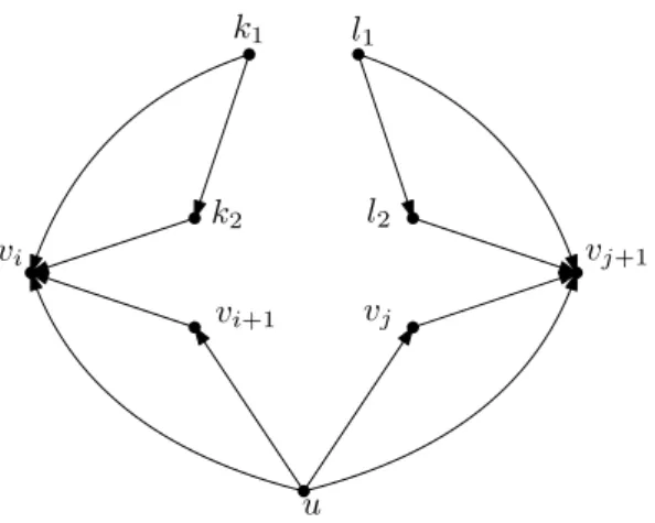
∀u∈V withS(u) = (v1, . . . , vm)∀1≤i < j < m:π(vi)< π(vi+1)∨π(vj)> π(vj+1) (2.1) As for a st-ordering π of a graph G for every edge (u, v) ∈ E, π(u) < π(v) by the definition, if for verticesk, l∈V a path exists fromkto l, then π(k)< π(l)has to hold.

Using the condition in Equation 2.2 and rewriting it as ¬(π(v_i) > π(v_i+1)∧π(v_j) <

π(v_j+1)), leads to the fact that if a path exists fromv_i+1 to v_i and a path exists fromv_j to vj+1 withi < j then no bitonic st-ordering can exist forG.

This combination of paths is referred to as forbidden configuration of paths. To characterise graphs that contain those forbidden configurations the following lemma is very useful.

Lemma 2.11. [Gro15] Let G = (V, E) a plane st-graph and F be the subgraph of G induced by a face that is not the outer face. For u, v∈F if a path exists fromu tov in G, such a path has to exist inF.

Proof. This has been proven several times, the idea Gronemann used is that if a path exists fromu tov that is not part of F it has to intersect either the paths from sto the face-source or from the face-sink totas can be seen in Figure 2.1b. In both cases a cycle is induced in contradiction to the st-planarity ofG.

(12)

u vi+1

v_i v_j vj+1

(a) [Gro15]A vertex u with successor list S(u) = (v₁, . . . , v_i, v_i+1, . . . , v_j, v_j+ 1, . . .) and a forbidden configuration of pathsv_i+1 v_i andv_j v_j+1.

s t

v

u F

(b) The path from uto v has to either intersect the path from the facesink tot or the path froms to the facesource.

Fig. 2.1.

Additionally it can be said that every face consists of two paths from the facesource sf to the facesink tf. As every face contains exactly two consecutive successors of the facesource v_j and v_j+1, the path containing v_j can be referred to as left path and the paths containingv_j+1 can be referred to as right path.

As consecutive members vi, vi+1 of a successor or predecessor list of a vertex u share a face with u, if a path exists from v_i to v_i+1 or from v_i+1 to v_i it has to exists on this face. Additionally because v_i is part of the left path of this face and v_i+1 is part of the left path, if there exists a path fromvi tovi+1, then vi+1 has to be the facesink and vice versa. If neither v_i norv_i+1 is the facesink no path can exist between them. Thus, we can test if a path exists between consecutive successors of a vertex u by looking at the sink of their common face withu.

Now that we established a forbidden configuration of paths, in an embedded planar st-graph, for it to admit a bitonic st-ordering and a way to test for the existence of those paths, we show that the absence of forbidden configurations is not only a necessary but a sufficient condition for a plane st-graph to admit a bitonic st-ordering.

First we have to prove the following lemma.

Lemma 2.12. [Gro15] Given an embedded planar st-graph and a vertex u ∈ V with successor listS(u) = (v1, . . . , vm). If it holds that

∀1≤i < j < m:vi+1 6 vi∨vj 6 vj+1

then there exists 1≤h≤m such that

(∀1≤i < h:vi+1 6 vi)∧(∀h≤ß< m:vi6 vi+1)

holds. In other words, there exists at least one vertexvh in S(u) whose preceding vertices inS(u)are only connected by path in clockwise direction, whereas paths between following vertices are directed counterclockwise.

(13)

v_h

u

v1 vm

Fig. 2.2.: [Gro15] The augmented graph G⁰ in the proof of Lemma 2.13 obtained by adding edges between consecutive successors ofu.

Proof. If there exists no path vi+1 vi with 1 ≤ i < m, we choose h = m. Then

∀1 ≤ i < m : v_i+1 6 v_i is satisfied. If there exists at least one such path, we set h=min{i|v_i+1 vi} to satisfy ∀1≤i < h:vi+1 6 vi by construction. Assuming that there exists a pathvj vj+1 withh≤j < m, there exists v_h+1 v_h and h≤j, which contradicts the assumption.

Lemma 2.13. [Gro15] Given a planar st-graph with a fixed embedding. If at every vertex v∈V with successor list S(u) = (v₁, . . . , v_m) the following holds:

∀1≤i < j < m:v_i+1 6 v_i∨v_j 6 v_j+1 then G admits a bitonic st-orderingπ.

Proof. This proof requires several steps. First an algorithm is described that inserts additional edges E⁰ into G. Those edges ensure that paths exist between all pairs of consecutive successors of all vertices of G⁰ = (V, E∪E⁰). Then it is proven that G⁰ is still planar and that any st-ordering ofG⁰ is a bitonic st-ordering ofG. For every vertex u ∈ V with successor list S(u) = (v1, . . . , vm), we can say by Lemma 2.12 that there exists a1≤h≤msuch that for every1≤i < hthere is no pathv_i+1 v_i, and for every h ≤i < m no pathv1 vi+1 inG. These edges can be added to create the two paths in v1 v2 · · · v_h ∈ G⁰ and vm vm−1 · · · v_h ∈ G⁰ as seen in Figure 2.2.

For every1≤i < mthree cases are to consider. If a path v_i v_i+1 or v_i+1 v_i exists between vi and vi+1 nothing has to be done. If no path exists betweenvi and vi+1 and i < h we add the edge (vi, vi+1) to E⁰ to ensure that π(vi) < π(vi+1). If no path exists between v_i and v_i+1 and h≤i < m we add the edge(v_i+1, v_i) so thatπ(v_i)> π(v_i+1).

Now we prove thatG⁰ is still a st-planar graph by induction over the number of added edges. We assume that E⁰ is in random order. Let G_k be the graph after inserting the first k edges into G. Clearly, G₀ is st-planar. When adding the k-th edge between two consecutive successors of a vertexu we may assume it is the edge(v_i, v_i+1) without loss of generality as the prove works symmetricaly with the edge (vi+1, vi). Let F be the subgraph induced by the common face ofu,v_i andv_i+1 inG. Withwbeing the facesink, the face consists of two paths u v_i w and u v_i+1 w. Because we insert an

(14)

edge neither v_i nor v_i+1 is the facesink. By our induction hypothesis we may assume thatGk−1 is still st-planar. As a maximum of one edge is added to each face in G,F is a subgraph of Gk−1, too. Thus planarity is preserved when inserting (v_i, v_i+1).

We now have to show thatG_kis still acyclic. SinceGk−1 is acyclic any cycle inG_khas to exist because of inserting the edge(vi, vi+1, thus has to contain the edge. This means that a path from vi+1 to vi has to exist in G_k, which has to have existed in Gk−1, too.

This is not possible, because the path would have had to exist on F by Lemma 2.11, contradicting the fact that vi is not the facesink. Thus every Gk is st-planar and it follows that G⁰ is st-planar.

Considering any st-ordering π of G⁰, because E⁰ ⊆E∪E⁰, π is an st-ordering for G.

As we constructedG⁰ in a way such that for everyu∈V withS(u) = (v1, . . . , vm), there exists a path vi vi+1 for 1≤i < hand a path vi+1 vi for h≤i < m. It follows for every st-orderingπ ofGthat

∀1≤i < h:π(vi)< π(vi+1)∧ ∀h≤i < m:π(vi)> π(vi+1).

In other words S(u) is bitonic increasing with respect to π for all u ∈ V. As G⁰ is st-planar at least one st-orderingπ of G⁰ has to exist.

This lemma does not only show that every graph without forbidden configurations admits a bitonic st-ordering, but also provides us with a linear time algorithm to find such an ordering.

For plane st-graphs that contain the forbidden configurations we introduced earlier, we cannot find a bitonic st-ordering. By splitting certain edges however, we can create a graph that admits a bitonic st-ordering. After drawing this graph we receive an upward planar drawing of the original graph, with edge bends. We introduce this procedure with an example. Let G = (V, E) be an embedded planar st-graph that contains a single forbidden configuration at one of its vertices u ∈V with S(u) = (v1, . . . , vm). Let this configuration be the two paths vi+1 vi and vj vj+1 withi < j.

By splitting the edge (u, v_i) or (u, v_j+1) we can augment G in a way that it admits a bitonic st-ordering. Let the split edge be (u, v_i) without loss of generality. Then a dummy vertex v_i⁰ is inserted and the edge is replaced by the edges (u, v_i⁰) and (v⁰_i, vi).

The successor list S(v⁰_i) contains only one element, namely v_i, thus it is bitonic with respect to every st-ordering. Additionally v_i⁰ replaced v_i in the successor list of u and because no path exists fromvi+1tov⁰_ithe forbidden configuration is resolved. By drawing the augmented graph and removing the dummy vertex, replacing it by a bend point for (u, v_i) we obtain an upward planar drawing of G with one bent edge. As we want to reduce the number of edge bends in the resulting drawing, we want to reduce the number of edge splits, when augmenting the graph G to let it admit a bitonic st-ordering. The following lemma shows that the number of edge splits is at most |V| −3.

Lemma 2.14. [Gro15] Every embedded planar st-graph G= (V, E) can be transformed into a new one that admits a bitonic st-ordering by splitting at most |V| −3 edges.

Proof. Considering a vertexu with successor listS(u) = (v₁, . . . , v_m)that contains mul- tiple forbidden configurations. Using the second condition in Lemma 2.12 we want to

(15)

|V| −3

Fig. 2.3.: [Gro15]Example of a pattern for graphs, with|V| −3forbidden configurations, each requiring one edge split to be resolved.

find a v_h such that every path between consecutive successors vi and vi+1, is directed fromv_i towardsv_i+1 fori < hand fromv_i+1 tov_iforh≤i < m. As due to the existence of forbidden configurations, this vertex does not exist, we have to split some edges. As- sumingv_h would be the first successor, so h = 1, every path vi vi+1 with 1≤i < m contradicts that choice. We can resolve this issue, by splitting every edge (u, v_i+1), for which this path exists. The maximum number of splits ism−1, if for every1≤i < ma path fromvi to vi+1 exists. AsGis acyclic, pathsvi vi+1 andvi+1 vi cannot exists at the same time. Thus, if the number of splits required this way would be more than

m−1

2 we can instead choseh=m and because we have less than ^m−1₂ paths of the form vi vi+1, the required amount of splits is less than vi vi+1. The sum P

u∈V |S(u)|

of the length of all successor lists is the number |E| of edges of G. Thus it holds that P

u∈V |S(u)|=|E| ≤3|V| −6. With m=S(u) in the former fraction, we get X

u∈V

|S(u)| −1

2 ≤ 3|V| −6− |V|

2 =|V| −3.

As the graph shown in Figure 2.3 requires |V| −3 edge splits, this upper bound for the maximum number of required edges splits for a planar st-graph to admit a bitonic st-ordering is tight. It is to note that the graph can be drawn upward planar in quadratic area without edge bends, while requiring the maximum amount of edge splits to admit a bitonic st-ordering. The algorithm that finds a minimum set of edges to split in linear time is explained in Section 3.2.1.

(16)

3. The augmented algorithm

In this chapter the algorithm is described that draws an upward planar graph by using the algorithm of Gronemann [Gro15] on the given graph and on its flipped graph. This idea is from Gronemann himself, who noticed that the pattern he introduced that matched his calculated maximum number of edge bends when using the algorithm, was easily drawable upward planar without any bends. The reason for that is the fact that the ability to find a bitonic st-ordering is depending on the successor list of each vertex, which are depending on the orientation of the given graph. For the upward drawings on the other hand the orientation of the graph is nearly irrelevant, as an upward drawing of a graphGcan be easily converted to an upward planar drawing of its flipped graphG. This˜ can be achieved by flipping the given graphGwith its drawing to get a downward planar drawing of G˜ and then mirroring the drawing on the x-axis to make it upward planar.

Before the new and thus implicitly the former algorithm by Gronemann is described in its details we prove that these steps actually lead to an upward planar drawing.

3.1. Correctness of the augmented algorithm

In this section we prove that the described procedure leads to an upward planar drawing of the given graph. First we show that flipping an upward planar drawing results in a downward planar drawing.

Lemma 3.1. Flipping every edge of a graph G = (V, E) and a corresponding upward planar drawing Γ results in a downward planar drawing Γ˜ of the flipped graph G.˜ Proof. Using the given definition of the flipped drawing of a graph it follows for every edge(v, u)∈E,˜ Γ˜_(v,u)(k) = Γ_(u,v)(1−k). It follows with0≤i≤j≤1 ⇐⇒ 0≤1−j≤ 1−i≤1 thatΓ˜^y_(v,u)(i) = Γ^y_(u,v)(1−i)>Γ^y_(u,v)(1−j) = ˜Γ^y_(v,u)(j). This is the definition of a downward planar graph, thus the claim stands.

Notice that because the operation of flipping is its own inverse, flipping a downward planar drawing, leads to an upward planar drawing. The next step is to show that mirroring a downward planar drawing on the x-axis results in an upward planar drawing.

Lemma 3.2. Mirroring a downward planar drawing of a graph G on the x-axis results in an upward planar drawing of G .

Proof. Let G = (V, E) upward planar graph and Γ an upward planar drawing of G.

Mirroring Γ on the x-axis results in a drawing Λ of G, with Λ^y(v) = −Γ^y(v) for every v∈V and withΛ^y_(u,v)(x) =−Γ^y_(u,v)(x)for all(u, v)∈E and all x∈[1,0]. Together with

(17)

a > b ⇐⇒ −a < −b and the definition of upward planar drawings, it follows: For all (u, v) ∈E and0≤i≤j≤1 : Λ^y_(u,v)(i) =−Γ^y_(u,v)(i)>−Γ^y_(u,v)(j) = Λ^y_(u,v)(j). ThusΛ is a downward planar drawing ofG.

Similar to Lemma 5.1, mirroring an upward planar drawing of a graph on the x-axis, results in a downward planar drawing of the graph because the process of mirroring is its own inverse.

The results of these two lemmas show that given an upward planar drawing of a graph Gwe can easily compute an upward planar drawing of the flipped graphG⁰ ofGby first flipping the drawing and then mirroring it on the x-axis.

3.2. Algorithm

In this section the enhanced algorithm for creating an upward planar drawing of a st- graphG is described. The pseudo-code of the described algorithms can be found in the appendix. The overall algorithm operates in the following steps:

• The minimum set of edges to split is computed forG and for its flipped graphG⁰. Whichever requires less splits to create a bitonic st-ordering is chosen.

• A bitonic st-ordering is computed for the chosen graph with its split edges.

• The coordinates of the vertices are computed, using the bitonic st-ordering and the algorithm by Gronemann. In case of the flipped graph being used, the coordinates changed, such that the resulting drawing is upward instead of downward planar.

• Create the actual drawing Γ by using the computed vertex positions and straight lines between the vertices as edges.

• Remove the dummy vertices, inserted at the split edges to make the drawing a drawing of the original graph, with bends.

In the following subsections we describe the most important steps of the algorithm.

3.2.1. Splitting the edges

The pseudo-code for this step can be found in Algorithm 1. In the first step the graph with the split edges which is used for creating the drawing is computed. First the minimum set of edges to be split is determined for the original graph with the algorithm by Gronemann. The algorithm is checking for each vertex v ∈V and its successor list S(v) = (v1, . . . , vm)which of its successors has to have the highest order in the bitonic st- ordering to require the least amount of splits. To describe this procedure some notation has to be introduced. Given a vertex u∈ V with successor list S(u) = (v₁, . . . , v_m) we define L(u, h) = |({i < h : vi+1 vi}| and R(u, h) = |{i < h : vi vi+1}|. When choosing a 1 ≤ h ≤ m for u, then every edge (u, v_i+1) with i < h has to be split if a

(18)

pathv_i+1 v_i exists, and every edge (u, v_i) with h ≤ihas to be split if Gcontains a pathvi vi+1. OverallL(u, h) +R(u, m)−R(u, h) edges have to be split. As R(u, m) does not change for different 1 ≤ h ≤ m, to find the minimum set of edges to split to resolve forbidden configurations for u we only have to consider L(u, h)−R(u, h) and minimise it. If a path vh vh+1 exists its follows that R(u, h+ 1) = R(u, h) + 1 and similarly L(u, h+ 1) = L(u, h) + 1 if a path vi+1 vi exists. Thus in the first case L(u, h+ 1)−R(u, h+ 1) = L(u, h)−R(u, h)−1 and L(u, h+ 1)−R(u, h+ 1) = L(u, h)−R(u, h) + 1. Because L(u,1)−R(u,1) = 0 to calculate L(u, h)−R(u, h) for every vertex we check for paths betweenvi andvi+1 iteratively for each i. After finding the 1 ≤h ≤m which requires the lowest amount of edge splits, it is computed, which of the edges actually have to be split to admit the ordering. After this is repeated for each vertex u, the minimum set of edges to be split is computed for the flipped graph the same way. The amount of splits required in both cases are compared and the case with the smaller number is chosen. For every edge(u, v) which has to be split, a dummy vertex w is inserted and (u, v) is replaced by (u, w) and (w, v). The resulting graph is then returned.

3.2.2. Computing the bitonic st-ordering

The pseudo-code for this step can be found in Algorithm 2. To find an bitonic st-ordering the graph is prepared in a way, such that every st-ordering is bitonic. In a bitonic st- ordering π of a graph the successor list S(v) of every vertex v ∈ V has to be a bitonic sequence. This means that for every S(v) = v1, . . . , vm there exist a 1 ≤ h ≤m, such thatπ(v_i)< π(v_i+1) and π(v_j)> π(v_j+1) for 1≤i < h≤j ≤m. As the used graph at this point has to admit a bitonic st-ordering this requirement is met for all neighbours in the successor list, which have paths between them. To ensure that neighbours in the successor list, which don’t have paths between them are ordered correctly, dummy edges are inserted. For this we iterate over all successors ofv and before we encounter a path vi vi+1we assume thati < hand thus for everyvi+1 6 viwe insert the edge(vi+1, vi), to ensure π(v_i) is higher than π(v_i+1). When for the first time there exists v_i v_i+1 we set h =i and fori > h if v_i 6 v_i+1, we insert the edge (v_i, v_i+1), to ensure π(v_i+1) is higher than π(vi). After repeating this procedure for every vertexv ∈V we compute a st-ordering using depth first search which is a bitonic st-ordering for G as shown in Lemma 2.13.

3.2.3. Obtaining the upward planar drawing

The pseudo-code for this step can be found in Algorithm 3. To obtain an upward planar drawing the algorithm provided by Gronemann [Gro16] is used. It is based on the algorithm by Harel and Sardas [HS98] to obtain a planar straight-line drawing, when given a biconnected canonical ordering, which in term uses a modified version of the algorithm by de Fraysseix et al. [DFPP90]. The original algorithm by de Fraysseix et al.

is using triangulated graphs for drawing and thus when a vertex is placed it has at least two neighbours that have already been placed. To avoid the step of triangulation for

(19)

a more pleasing visualisation Harel and Sardas introduced the property of having left, rights and legal support, for vertices that only have one preceding neighbour. To apply those properties to bitonic st-orderings dummy verticesv_Landv_Rare added that take the roles ofv₁ andv₂in the original algorithm. The algorithm only computes the coordinates of the vertices, as the edges are represented as straight lines and follow implicitly.

(20)

4. A new lower bound

Now after the algorithm has been introduced in the previous chapter the question arises wether additionally considering the flipped graph actually lowers the upper bound of the maximum number of edge splits. While it is obvious that the number of required splits is lower for some graphs, it might be possible that the upper bound does not improve at all. In this chapter we first introduce a simple pattern of graphs derived from the former worst case, to get a lower bound for the maximum number of required splits. This pattern leads to an observation on how to create patterns which require a high number of splits for both orientations of the graph. Using this the pattern of our worst case example so far is introduced.

Given the example of Gronemann [Gro15], for graphs which require exactly |V| −3 edge splits, matching the upper bound, the idea for a new bad pattern is to take the old pattern two times, one time in the original, one time with flipped edges and connecting their sinks and sources, as can be seen in Figure 4.1b, creating one graph with twice the amount of vertices. As the old pattern is included in the graph and because stays the same when flipping it requires|V| −3splits in both directions while having2|V|vertices.

Withn= 2|V|this results in a graph withnvertices which requires n/2−3 edge splits in both orientations.

Using the same method we notice that given a graphG= (V, E)we can always create a graph which has 2|V| vertices and its required number of splits is the sum of the number of splits required forGand for the flipped graph ofG. Compared to the number of vertices of each graph the new graph requires approximately the average number of splits thatGand its flipped graph require in both orientations. In the following lemmas this will be proven and the exact number of splits required to find a bitonic st-ordering or a bitonic ts-ordering is calculated.

Lemma 4.1. Given two plane graphs G₁ = (V₁, E₁) and G₂ = (V₂, E₂), which require k₁ and k₂ edge splits to admit a bitonic st-ordering andl₁ and l₂ edge splits to admit a bitonic ts-ordering, a new graph G = (V, E) can be created, with |V| = |V₁|+|V₂| and which requiresk₁+k₂ splits to admit a bitonic st-ordering and l₁+l₂ edge splits to admit a bitonic ts-ordering.

Proof. The Lemma is proven by uniting the two given graphs and inserting the two edges (s2, s1)and(t2, t1)to make the resulting graphG= (V1∪V2, E1∪E2∪ {s₂, s1} ∪ {t₂, t1}) a st-graph with source s=s₂ and sink t=t₁. This is visualised in Figure 4.1a.

Because new edges have been added, the embedding, which is represented by the successor and predecessor list of each vertex, has to be updated. For s1 its new and only predecessor s₂ is added as only vertex in the predecessor list and for t₂ the new

(21)

s₂ t2

t1

s1

G₁ G₂

(a) Overall graph after uniting procedure from Lemma 4.1

t

s

|V| −3

(b) Example of a graph withnvertices needing n/2−3 edge splits in both directions

successor t1 is added to the successor list. Fors2 and t1 the verticess1 and t2 are added as new first members in the successor and predecessor lists.

This way, every pair of vertices which appears consecutively in the successor list or predecessor list of any vertex still appears consecutively in the new successor and predecessor lists. Thus we can ensure that configurations that require edge splits for admitting a bitonic st-ordering or bitonic ts-ordering still appear in the same way in the united graph.

Using this method of uniting two graphs with the same number of verticesn=|V₁|=

|V₂|, which requirek1 and k2 splits to admit a bitonic st-ordering as above, the resulting graph G = (V, E) has 2n vertices and requires k₁ +k₂ splits to admit a bitonic st- ordering. The number of splits required relative to the number of vertices of the graph is(k1+k2)/2n. This is the mean of the relative number of splits thatG1 andG2 require to admit a bitonic st-ordering. Similarly the relative number of splits required to admit a bitonic ts-ordering is(l₁+l₂)/2n.

Lemma 4.2. Given a plane graph G = (V, E) which require k edge splits to admit a bitonic st-ordering and l edge splits to admit a bitonic ts-ordering, a plane graph G⁰ = (V⁰, E⁰) can be found, with |V⁰| = 2|V| which requires k+l splits to admit a bitonic st-ordering or a bitonic ts-ordering.

Proof. Using Lemma 4.1 withGand its flipped graphG˜ leads toG⁰.

As the graph that is described in this lemma stays the same when flipped it requires the same number of edge splits to admit a bitonic st-ordering or a bitonic ts-ordering.

This means that in order to find a graph that requires a high amount of splits both to admit a bitonic st-ordering and a bitonic ts-ordering, not only a graph where the lower number of splits required for the graph to admit one of the orderings, but the mean of them.

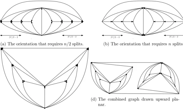
The worst case pattern that we could find is the pattern seen in Figure 4.2. This pattern leads to a lower bound for the maximum number of required edge bends when creating an upward planar drawing of a directed graph G in quadratic area with the given algorithm.

(22)

|V|/2−2 |V|/2−2

(a) The orientation that requiresn/2splits.

|V|/2−2 |V|/2−2

(b) The orientation that requiresnsplits.

(c) The pattern that requiresn/2splits drawn upward planar.

(d) The combined graph drawn upward planar.

Fig. 4.2.: Our worst case example in both orientations.

Theorem 4.3. There exist graphs that require 3/4|V| −3 edge splits to admit a bitonic st-ordering or a bitonic ts-ordering.

Proof. The pattern shown in Figure 4.2 requires 2∗(|V⁰|/2−2) = |V| −4 splits to admit a bitonic st-ordering and|V⁰|/2−1splits to admit a bitonic ts-ordering. Using the procedure described in Lemma 4.1, a graph with |V|= 2|V⁰| is created which requires

|V|/2−2 +|V|/4−1 = 3/4|V| −3edge splits in both orientations, thus a upward planar drawing is found with the given algorithm with 3/4|V| −3 edge bends.

As this pattern is requiring |3/4| −3 edge splits to admit a bitonic st-odering or a bitonic ts-ordering it also provides a lower bound for the maximum number of edge splits when creating an upward planar drawing with our algorithm. Progress that we have made on the way to finding a new upper bound is described in the next chapter.

(23)

5. Towards upper bounds

To find out if the updated algorithm is better than the previous algorithm of Gronemann in a meaningful way, a new upper bound for the maximum required number of edge splits to admit a bitonic st-ordering has to be found.This chapter is about different observations that have been made in the search of this new upper bound. While we were not able to find a new upper bound the results of this chapter might prove useful on the way to establishing a new upper bound. In Section 5.1 we show that it suffices to consider triangulated graphs when looking for a new upper bound. Section 5.2 focuses on different observation about the degrees of vertices. In Section 5.3 two different directions for finding a new upper bound are outlined.

5.1. The worst case is a triangulation

In Lemma 2.11 we showed that if a path exists between consecutive successors vi, vi+1

of a vertex u, it has to exist on the face the three vertices share. As u is the only source of this face we can consider forbidden configurations as forbidden configuration of faces instead of paths. One path and thus the corresponding face can form a forbidden configuration with different faces, which are then all resolved by splitting the transitive edge of that face. To account for that, when counting the required edge splits for certain graphs it is a useful model to think of it as pairing faces together, which form forbidden configurations. The linking of paths that form a forbidden configuration to the faces they share with the vertex they form the configuration for leads to the following observation.

Lemma 5.1. All but one of the inner faces have to be involved in a forbidden configuration to reach the maximum number of required splits.

Proof. Letu∈V be a vertex with successor listS(u) = (v1, . . . , vm) and vi+1 vi and vj vj+1 with i < j a pair of paths that form a forbidden configuration. Because u is always the source of the faces thatv_i, v_i+1, uand v_j, v_j+1, ushare respectively, and as faces have only one source in st-graphs, we need two faces for a forbidden configuration and those faces can’t be part of a forbidden configuration of any other vertex. Using the maximum number of faces and the fact that the outer face is never part of a forbidden configuration, we have 2|V| −5 faces left. The upper bound of forbidden configurations is |V| −3. As two faces are needed for any one of these configurations, 2|V| −6 faces are needed to create the maximum number of forbidden configurations. This leaves one inner face that is not part of any such configuration.

As this lemma applies to the graph G as well as its flipped graph G, all but two˜ inner faces have to be part of a forbidden configuration in both orientations for the old

(24)

maximum to be met.

This lemma implies that for a graph to require the maximum amount of edge splits it has to be triangulated. While the maximum number of required edge splits for a graph with the updated algorithm might be lower than |V| −3 and thus we cannot assume that a graph meeting this number is triangulated we can still limit our observations to triangulated graphs as the following lemma shows.

Lemma 5.2. Given a graph G = (V, E) any triangulation G⁰ = (V, E⁰) of G needs at least as many edge splits to admit a bitonic st-ordering as G.

Proof. We prove that for every vertexv∈V the required amount of edge splits, to admit a bitonic ordering of its successors, does not get smaller. LetS(u) = (v₁, . . . , v_m)be the successor list of u. If all faces that have u as source are triangulated already, the faces incident to all pairs of successors ofvi, vi+1,1≤i≤m−1 and u don’t change and the number of required splits stays the same.

As the only faces that are relevant for forbidden configurations foruare faces incident to consecutive successorsv1, vi+1ofuwhere there exists a pathvi vi+1orvi+1 viwe have to prove that similar faces exist after the triangulation. Without loss of generality we can assume that the path is a path from v_i to v_i+1. If after triangulating an edge exists between vi and vi+1 it has to be the edge (vi, vi+1) because else there would be a cycle. If this edge doesn’t exist after the triangulation at least one new successor has been added to the successor list of u between v_i and v_i+1. Let the first of these new successors be the the vertexv⁰_i+1. This vertex was incident to the same face as vi, uand v_i+1 before the triangulation. As the graph is triangulated now there has to be an edge between v_i and v⁰_i+1. As v⁰_i+1 was part of the path v_i v_i+1 before the triangulation that edge has to be the edge(vi, v_i+1⁰ ).

As for the old upper bound to stand the graph has to be a triangulation, we can say for every forbidden configuration that exists that between the faces of the forbidden configuration there are no other faces except for pairs that are a forbidden configuration themselves.

5.2. Different observations on vertex degrees

In this subsection we focus on different observations that were made regarding vertex degrees. Looking at a Vertex u with one forbidden configuration, we already noticed that it has to be the source of two faces. The sinks of these faces are different successors of u. This means for the faces to be part of forbidden configurations after flipping the graph they have to be newly paired. Thus getting a new upper bound by looking at bad configurations for each vertex separately is impossible.

In the attempt to further characterise the graphs that are able to reach |V| −3 splits in both directions the following observations have been made.

Lemma 5.3. If the number of successors |S(u)| of a vertex u ∈V is even at least one face that hasv as its source, is not part of a forbidden configuration.

(25)

Proof. We are using the same arguments that were used in the proof of Lemma 2.14. Let S(v) = (v1, . . . , vm) be the successor list of u. For S(u) = (v1, . . . , vm) to be a bitonic sequence with respect to an orderingπ a vertexv_h,1≤h≤mhas to exist, such that for consecutive successors v_i, v_i+1 of u there is no path from v_i+1 to v_i for i < h and there is no path from vi to vi+1 for i≥ h. If those paths exist we can resolve it by splitting edges. Assuming for v_h to be the first successor. Then every path from vi to vi+1 for 1≤i≤m−1, forces the edge(u, v_i+1)to be split. If we chosev_h to be the last successor of u, then every path from vi+1 to vi forces the edge (u, vi) to be split. As G is acyclic pathsvi vi+1 andvi+1 vi cannot exist simultaneously. Thus if more than ^m−1₂ path exist fromv_i tov_i+1, less than ^m−1₂ paths fromv_i+1 tov_i can exist. Thus the maximum number of splits at each vertex is at most ^m−1₂ for each vertex. Ifm is even, the biggest natural number that is at most ^m−1₂ is ^m−2₂ .

As every vertex butsandthave at least one predecessor and one successor and because we have to consider the flipped graph two, the vertex degree of every except forsand t has to be even if all faces should be paired. This leads to the following lemma.

Lemma 5.4. The degree of each vertex but s and t has to be even for all faces to be paired in forbidden configurations.

Proof. As predecessors and successors are exchanged when flipping, and because as shown in Lemma 5.3 the number of successors have to be odd for every face to be paired, both the number of predecessors and the number of successors have to be odd for each face to be paired. Thus degree of the vertex which is the sum of its number of successors and predecessors is even.

This means for the old upper bound to stand, only a constant amount of vertices can have odd degree. As for planar graphs the average degree of each vertex is less than six and because in a triangulated graph every vertex has at least degree 3, at most half of the vertices can have a degree higher than six.

To take a further look on local patterns the following lemma is very useful.

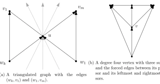
Lemma 5.5. In a triangulated graph G = (V, E) for every vertex u with S(u) = (v₁, . . . , v_m)andP(u) = (w₁, . . . , w_k)that is not the source or the sink, the edges(w_k, v₁) and(w1, vm) have to exist in E.

Proof. As the graph is triangulated for every pair of consecutive neighbours of each vertex, there has to be an edge between those vertices. It can be seen in Figure 5.1a that the paths w_k v₁ and w₁ v_m exist, thus the orientation of these edges have to be (w_k, v₁) and(w₁, v_m).

For vertices of degree four, which require an edge split in the current orientation, thus have three successors, this leads to configuration that can be seen in Figure 5.1b. If the only predecessor of a degree four vertex is another degree four vertex, which has a degree four vertex as its only predecessor and so on, this leads to a pattern which can be seen in Figure 5.2a that is similar to the worst case pattern that Gronemann [Gro15] introduced

(26)

u

v₁ vm

w_k w₁

(a) A triangulated graph with the edges (w_k, v₁)and(w₁, v_m).

v

(b) A degree four vertex with three successors and the forced edges between its predecessor and its leftmost and rightmost successors.

Fig. 5.1.:The observation from Lemma 5.5 leads to a specific pattern for degree four vertices.

that is shown in Figure 2.3. This means that if degree four vertices are grouped together it also leads to two vertices, which are incident to all those vertices and thus have a degree equal to the number of degree four vertices in this section of the graph. When considering the flipped graph, those two vertices are now the sources of all the faces incident to the degree four vertices. No edge splits are required in this orientation for those faces as the successors are sorted in ascending and descending order respectively. Thus for all faces to be part of forbidden configurations, additional vertices have to be added. Looking at the right successor w of the degree four vertices in the original orientation, for all the faces to be part of a forbidden configuration in the flipped case, an equal number of successors has to be added, where the edge between consecutive members of these successors has to be the reversed direction of the edges between the degree four vertices, with respect to the successor list of w. This is shown in Figure 5.2b. Using the same arguments to add faces to the left half of this pattern, leads to an overall pattern which resembles our worst case introduced in Theorem 4.3. Thus it seems probable, that a graph with a lot of degree four vertices cannot require a higher amount of splits than our example. If this could be proven the only other case that would have to be studies is a graph with many degree six vertices as the average degree in planar graphs is lower than six and we showed that the majority of vertices have to have even degree for the graph to require a large amount of splits.

5.3. Future work

This section is about future research that can be done on this algorithm. One way to go is to prove wether the algorithm has a lower maximum number of edge bends than the old algorithm that did not consider bitonic ts-orderings. As all but one face are part of a forbidden configuration to reach|V| −3edge bends, this means that all but two faces have to be part of a forbidden configuration in both orientations of the graph. Thus, if