On the avoidance of crossing of singular values in the evolving factor analysis.
Klaus Neymeyra,b, Mathias Sawalla, Zahra Rasoulic, Marcel Maederd
aUniversit¨at Rostock, Institut f¨ur Mathematik, Ulmenstrasse 69, 18057 Rostock, Germany
bLeibniz-Institut f¨ur Katalyse, Albert-Einstein-Strasse 29a, 18059 Rostock
cInstitute for Advanced Studies in Basic Sciences, 45195-1159 Zanjan, Iran
dUniversity of Newcastle, Department of Chemistry, Callaghan, NSW 2308, Australia
Abstract
Evolving factor analysis (EFA) investigates the evolution of the singular values of matrices formed by a series of measured spectra, typically, resulting from the spectral observation of an ongoing chemical process. In the original EFA the logarithms of the singular values are plotted for submatrices that include an increasing number of spectra. A typical observation in these plots is that pairs of trajectories of the singular values are on a collision course, but finally the curves seem to repel each other and then run in different directions. For parameter-dependent square matrices such a behaviour is known for the eigenvalues under the keyword of an avoidance of crossing. Here we adjust the explanation of this avoidance of crossing to the curves of singular values of EFA. Further, a condition is studied that breaks this avoidance of crossing. We demonstrate that the understanding of this non-crossing allows us to design model data sets with a predictable crossing behaviour.
Key words: evolving factor analysis, EFA plot, avoidance of crossing
1. Introduction
The rank of a spectral data matrix Dcan be estimated by the number of above-noise-level eigenvalues of the symmetric matrixDTD. In many chemical applications the rows of the data matrix are formed by a series of spectra taken as a function of time or generally of process progress. ThereinDis ak-by-nmatrix, wherekis the number of spectra andnthe number of wavelengths at which the spectra are measured. In such instances the rank is often seen as the chemical rank or the number of linearly independent species that co-exist in the process under investigation. In Evolving Factor Analysis, EFA, the development of the rank can be further analysed by determination of the rank of submatrices ofD. EFA was first introduced by Gampp et al. [1] and was improved by Maeder and coworkers [2, 3, 4].
It has found a large number of applications in various fields of analytical chemistry as a model-free method for fast information extraction. Typically, the data is recorded from ongoing chemical reactions, chromatographic processes, spectrophotometric titrations or processes that are subject to change under varying parameters as temperature, pH values or time [5].
In the original EFA the submatricesD[ℓ] are formed by a growing number of rows ofD, starting with the first, then the first two, then the first three rows, etc.
D[ℓ] :=D([1 :ℓ],:)∈Rℓ×n (1)
forℓ = 1, . . . ,k. In other words, theD[ℓ] are sub-matrices of thek×nmatrixD. A possible interpretation is that Dcontains the full spectral observation of a chromatographic experiments and the D[ℓ] reflect the progress of the measurement.
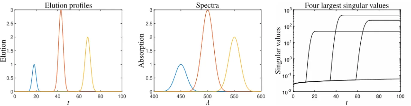
In order to introduce the topic of the present paper let us consider the following three-component chromatographic data set. On the wavelength intervalλ∈[400,600] we take the three spectral profiles
s1(λ)=g(λ,450,30), s2(λ)=3g(λ,500,30), s3(λ)=2g(λ,550,30) (2) with the Gaussiang(λ,a,b) = exp(−(λ−a)2/(b/2)2). The elution (concentration) profiles on the time intervalt ∈ [0,100] are supposed to be
c1(t)=g(t,36,5), c2(t)=3g(t,43,6), c3(t)=2g(t,46,7). (3) These profiles are shown in Figure 1. The functions are discretised by usingδλ=0.25 andδt =0.1. This yields a matrixS ∈R801×3of spectral profiles and a matrixC ∈R1001×3of elution profiles. Thus the absorbance data matrix
0 20 40 60 80 100 0
0.5 1 1.5 2 2.5
3 Elution profiles
t
Elution
400 450 500 550 600
0 0.5 1 1.5 2 2.5
3 Spectra
λ
Absorption
0 20 40 60 80 100
10-2 10-1 100 101 102
103 Four largest singular values
t
Singularvalues
36 38 40 42 44 46 48
30 40 50 60 70 80 90 100
Four largest singular values
t
Singularvalues
Figure 1: Top row: Elution profiles of the three components and their spectra. Lower row: The 4 largest singular values ofD[ℓ] forℓ=1, . . . ,100.
The curves of the three largest singular values do not intersect which is indicated by the sectional enlargement in the lower right subplot.
D=CSTis a 1001×801 matrix. We add about 0.1 percent (of the maximal absorption) normal distributed noise with the mean 0 and the variance 1.
If no noise is added and ifℓ≥3, the rank of all theD[ℓ] equals 3. If 0.1 percent of noise is added, then the fourth and all following eigenvalues are close to zero. Figure 1 shows in its lower row the four largest singular values ofD[ℓ]
forℓ=10tandt=0.1,0.2, . . . ,100. The curves of the three largest singular values show the typical behaviour, they seem to follow the concentration profiles of the three species and appear to be on collision course with another curve, but finally the curves seem to repel each other. This repulsion is clearly shown by the sectional enlargement in the lower right plot of Figure 1. This behaviour of the curves of singular values is typical of most of the EFA curves and can be found in many of such plots in the referenced paper on EFA. A mathematical explanation for this non-crossing of the singular value curves is given in the next section.
2. Avoidance of crossing
First, the avoidance of crossing of the eigenvalues of a parameter-dependent matrix is illustrated by
C(α) :=(1−α)A+αB (4)
for symmetric matricesAandBand with a real parameterα. Symmetry of the matrices is essential for the following analysis; later we connect the singular values ofD[ℓ] with the square roots of the eigenvalues of the symmetric matrix D[ℓ]TD[ℓ]. Figure 2 shows the eigenvalues ofC(α) for a more or less random choice of symmetric 2×2 matricesA andBagainstα∈[0,1.5]. Starting atα=0 the two eigenvaluesλ1(α) andλ2(α) are getting closer for increasingα, but then show the typical behaviour of a mutual repulsion. Aroundα=0.55 the difference of the eigenvalues is the smallest and after this the distance monotonously increases. This phenomenon is known under the keywords of an avoidance of crossingornon-crossing. It was observed in quantum mechanics for parameter dependent Hamiltonian operators and was investigated by Wigner and von Neumann [6]. The eigenvalue non-crossing of symmetric matrices is closely related to the question how likely a symmetric matrix with random matrix elements has multiple eigenvalues.
To our knowledge the best explanation in a linear algebra textbook was given by Lax in Section 9.5 of [7].
Next we recapitulate the argumentation by Lax that is based on a study of the likelihood that an arbitrary symmetric matrix has a degenerate eigenvalue, namely an eigenvalue of the multiplicity 2. First, we state that a symmetricn×n matrix hasn(n+1)/2 degrees of freedom (dof). These are the number of its matrix elements that can independently be assigned by real numbers; its sub-diagonal elements determine its super-diagonal elements by symmetry. There is
0 0.5 1 1.5 -4
-2 0 2 4
6 Avoidance of eigenvalue crossing
α
Eigenvalues
Figure 2: Avoidance of crossing of the two eigenvalues ofC(α) forα∈[0,1.5] and the symmetric 2×2 matricesA=1
2 2 4
,B=2
−2
−2 2
.
a second way to count these dof by considering the eigenvalue/eigenvector decomposition of the symmetric matrix.
Therefore we count the dof of the eigenvalues and the associated eigenvectors. If all eigenvalues of the matrix are simple, then we have n dof for the eigenvalues. The associated eigenvectors form an orthogonal matrix and are normalized. Hence, the first eigenvector hasn−1 dof (namely for the components of the eigenvector and where the last component is determined by the normalization constraint), the secondn−2 and the second to the last 1 dof. The step-wise reduced number of dof is a consequence of the orthogonality relations between the eigenvectors. Summing up all these dof we get
|{z}n
dof of eigenvalues
+ (n−1)+(n−2)+. . .+1
| {z }
dof of eigenvectors
=n(n+1) 2 =:N.
In the case of a degenerate matrix with an eigenvalue with the multiplicity 2 and all remaining eigenvalues being simple, the latter summation is to be modified as follows: First, onlyn−1 eigenvalues can be chosen. If we start by counting the dof of the eigenvectors associated with the simple eigenvalues, the argumentation is as above. If we reach the second to the last and the last eigenvector that belong to the degenerate eigenvalue, then the eigenspace is completely determined and no dof remains. Thus we get
n−1
|{z}
dof of eigenvalues
+ (n−1)+(n−2)+. . .+2
| {z }
dof of eigenvectors
=n(n+1)/2−2=N−2
degrees of freedom. NextC(α) is considered as a curve depending on the parameterα. (In order to follow this geometric interpretation, imagine the example of the parameter-dependent vectorc(α)=(sin(α),cos(α))T that forms a circle in the two-dimensional space forα∈[0,2π].) As it is unlikely for the curveC(α) in theN-dimensional space to hit a surface that depends onN−2 parameters, the avoidance of crossing is a typical behaviour for eigenvalues. (In order to illustrate the last argument, consider the 2×2 matrix (4) that hasN =3 degrees of freedom. ThenC(α) is a curve in a three-dimensional space for which it is unlikely to hit a surface with the dimensionN−2=1, namely a second curve. Metaphorically speaking two randomly moving helium atoms in an evacuated vessel will nearly never collide.)
This explains the observed non-crossing of the three largest singular values of the EFA matrixD[ℓ] as considered in Section 1. These singular values are the square roots of the eigenvalues of the symmetric matrixD[ℓ]TD[ℓ]. In the noise-free case then×nmatrixD[ℓ]TD[ℓ] has three nonzero eigenvalues andn−3 zero eigenvalues. If noise is added, then the latter eigenvalues are close to zero. The non-crossing argumentation applies to the eigenspace that is spanned by the eigenvectors belonging to the nonzero eigenvalues.
3. Forcing a crossing of the singular values/eigenvalues
In some cases the crossing of eigenvalues can be forced [8]. By the following example we show that pairwise (approximate) orthogonal elution profiles seem to constitute an eigenvalue crossing. Therefore, we reuse the model problem from Section 1 but increase the mutual distances of the centres of the the elution profiles (3). So we consider the nearly orthogonal profiles
c1(λ)=g(λ,18,5), c2(λ)=3g(λ,43,6), c3(λ)=2g(λ,68,7) (5) The spectra are still given by (2). The numerical results are shown in Figure 3 withδλ=0.2 andδt=0.1. A sectional enlargement of the crossing point cannot confirm an avoidance of crossing. The curves of singular values are drawn
0 20 40 60 80 100 0
0.5 1 1.5 2 2.5
3 Elution profiles
t
Elution
400 450 500 550 600
0 0.5 1 1.5 2 2.5
3 Spectra
λ
Absorption
0 20 40 60 80 100
10-2 10-1 100 101 102
103 Four largest singular values
t
Singularvalues
Figure 3: Case of nearly orthogonal elution profiles. Then a crossing of the singular values seems to be taking place at a first rough glance. The singular value curves are drawn in black in order to avoid a preliminary interpretation concerning potential non-crossing.
0 20 40 60 80 100
0 0.5 1 1.5 2 2.5
3 Elution profiles
t
Elution
400 450 500 550 600
0 0.5 1 1.5 2 2.5
3 Spectra
λ
Absorption
0 20 40 60 80 100
10-2 10-1 100 101 102
103 Four largest singular values
t
Singularvalues
Figure 4: Case of nearly orthogonal elution profiles but strongly overlapping spectra. Once again, an avoidance of crossing of the singular values can be observed.
as black lines in order not to imply a certain behaviour. However, the numerical resolution is limited as we do not have a parameter-dependent problem like (4) that depends on a continuous changeable parameter. Instead, the time axis is discretised by the parameterδtwhich limits the maximal resolution.
However, there is still a non-neglectable influence of the spectra. If we use the orthogonal profiles (5) but modify the spectra (2) from Sec. 1 in a way of a stronger overlap to
s1(λ)=g(λ,490,30), s2(λ)=3g(λ,500,30), s3(λ)=2g(λ,510,30), (6) then the avoidance of crossing of the singular values can be observed, see Fig. 4. We conclude that an orthogonality of the spectra and additionally an orthogonality of the elution profiles result for these problems in a true singular value crossing. And in fact, the following mathematical analysis shows that the orthogonality of the spectra together with the orthogonality of the elution profiles are sufficient conditions that make an eigenvalue crossing possible.
If eachC andS have orthogonal columns, which are not necessarily orthonormal, then these matrices can be represented as
C=[c1, . . . ,cm]=Pdiag(kc1k, . . . ,kcmk)
| {z }
DP
,
S =[s1, . . . ,sm]=Qdiag(ks1k, . . . ,ksmk)
| {z }
DQ
with orthonormal matricesP∈Rk×mandQ∈Rn×mand diagonal scaling matricesDPandDQ. ThenPandQsatisfy PTP=Im×m and QTQ=Im×m.
By direct calculation we get that
DTD=(CST)TCST =(PDP(QDQ)T)TPDP(QDQ)T =QD2PD2QQT, DDT=CST(CST)T =PDP(QDQ)T(PDP(QDQ)T)T =PD2PD2QPT or equivalently
DTDQ=QD2PD2Q, DDTP=PD2PD2Q.
If we denote theith column ofQbyqiand theith column ofPbypi, then the last equations can be rewritten as DTDqi=kcik2ksik2qi, DDTpi=kcik2ksik2pi fori=1, . . . ,m.
This means that the eigenvectors ofDTDare the columnsqiofQand that the associated eigenvalues arekcik2ksik2. Similarly, thepiare the eigenvectors ofDDT.
Thus the singular value of Dthat is associated with qi iskcik · ksik, namely the square root ofkcik2ksik2. We conclude that theith EFA singular valueσiaccording to the matricesD[ℓ] by (1) of growing dimension equals
σi=kci(1 :ℓ)k · ksikfor ℓ=1, . . . ,k. (7)
This means that the singular value curve of theith singular value is only determined by itsith concentration profile ci and its time developmentci(1 : ℓ) as well by its associated spectrumsi. The other profilescjandsjfor j ,ido not affect theith singular value. This implies that these singular value curves can cross - they completely ignore the behaviour of the other singular values.
IfC andS have orthogonal columns, then the singular value curves can cross. However, we do not claim the reverse statement, namely that for non-orthogonal matrices a crossing is impossible. Assuming, the existence of crossing curves in the case of non-orthogonality, the avoidance of crossing rule shows that arbitrarily small changes of such a system will nearly always change the singular values in a way so that its curves are on a non-crossing course.
In the language of mathematics, the set of matrices with multiple singular values is of the measure zero in the set of all matrices. Such cases are not accessible numerically in the presence of rounding errors or for experimental data with its limited data precision.
4. Design of model systems with a predicted crossing behaviour of the singular values
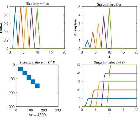
The analysis in Section 3, which determines theith singular value of EFA to be given by (7), allows us to design a model system with a completely predictable behaviour of the curves of singular values. Next, we substitute the Gaussian profiles by simple triangle profiles with their compact supports. The advantage of such profiles is that the orthogonality constraint can easily be implemented. Contrastingly and in a strict mathematical sense, a pair of Gaussian profiles can never be orthogonal, but can only be close to be orthogonal if the centres of the Gaussians are well separated.
Next four model problems are considered with each five chemical components. The elution profiles and the spectra of these components are modeled by triangle profiles.
Experiment I:The centres of the elution profiles are att =2,4,6,8,10 and the supports of the triangle profiles do not overlap. The maximal elution equals 1 for all components. The spectra are centred atλ =2,4,6,8,10, and the maximal absorption values are linearly increasing, see Fig. 5 for all these profiles. Further, Fig. 5 shows the sparsity pattern ofDTD, namely the so-called spy-plot in Matlab. Its structure is that of a block diagonal matrix in accordance with the analysis in Sec. 3. The curves of singular values show the typical crossing behaviour - each curves crosses all other curves.
Experiment II:Compared to the first experiment, we move the elution profile of the third component along thet-axis so that the orthogonality with the elution profile of the fourth component is broken. The spectra are the same as in the first experiment. Fig. 6 shows the profiles, the sparsity pattern ofDTDand the curves of singular values. Now DTDis a matrix with only four diagonal blocks with a joint block for the third and fourth component with doubled dimensions. Consequently, the curves of the singular values (drawn in ochre and purple) show the typical avoidance of crossing behaviour.
Experiment III:Compared to the first experiment, we reverse the growth pattern of the maximal absorption of the spectral profiles. Now these maximal values are linearly decreasing, see Fig. 7. The sparsity pattern is the same as in the first experiment. The curves of singular values are forced to develop in a well separated way. The question of a crossing or an avoiding of crossing does not arise.
Experiment IV:In contrast to the setup of the third experiment, we set the maximal absorption value of the fifth component to the largest value compared to the other components. The sparsity pattern ofDTDremains to be that of a block diagonal matrix. However, the curve of singular values of the fifth component is forced to cross the curves of the singular values of all other components, see Fig. 8.
In these four experiments we have in three cases modified the spectra and in one case we have forced the con- centration profiles to overlap. There is no need to make further experiments in which these modifications are applied to the other factor. This will not provide new results. The reasoning is as follows: First, a transposition applied to the spectral data matrixD =CST results inDT =S CT so thatCandS change their places. If it is true thatDand DT have the same (nonzero) singular values, thenC andS have a comparable influence on the singular values. In order to show this letD = UΣVT be a singular value decomposition ofD. ThenDT =VΣTUT is a singular value
0 5 10 15 20 0
0.2 0.4 0.6 0.8 1
0 5 10 15 20
0 1 2 3 4 5
0 100 200 300
nz = 4500 0
100
200
300
0 5 10 15 20
0 10 20 30 40 50
Elution profiles
Elution Absorption
Spectral profiles
Sparsity pattern ofDTD Singular values ofD
t
t λ
Figure 5: Model problem I with five components. Orthogonal elution profiles and orthogonal spectra. Increasing absorption values (first component with lowest absorption and last component with highest absorption) result in a maximal crossing of the curves of the singular values.
0 5 10 15 20
0 0.2 0.4 0.6 0.8 1
0 5 10 15 20
0 1 2 3 4 5
0 100 200 300
nz = 6300 0
100
200
300
0 5 10 15 20
0 10 20 30 40 50
Elution profiles
Elution Absorption
Spectral profiles
Sparsity pattern ofDTD Singular values ofD
t
t λ
Figure 6: Model problem II. Compared to the model problem I, the elution profiles of third and fourth component are forced to overlap. Conse- quently, the associated curves of singular values in ochre and purple show the typical avoidance of crossing.
0 5 10 15 20 0
0.2 0.4 0.6 0.8 1
0 5 10 15 20
0 1 2 3 4 5
0 100 200 300
nz = 4500 0
100
200
300
0 5 10 15 20
0 10 20 30 40 50
Elution profiles
Elution Absorption
Spectral profiles
Sparsity pattern ofDTD Singular values ofD
t
t λ
Figure 7: Model problem with five components. Orthogonal elution profiles and orthogonal spectra. Decreasing absorption values (first component with highest absorption and last component with lowest absorption) result in well separated non-crossing curves of the singular values.
0 5 10 15 20
0 0.2 0.4 0.6 0.8 1
0 5 10 15 20
0 2 4 6
0 100 200 300
nz = 4500 0
100
200
300
0 5 10 15 20
0 10 20 30 40 50 60
Elution profiles
Elution Absorption
Spectral profiles
Sparsity pattern ofDTD Singular values ofD
t
t λ
Figure 8: Model problem with five components. Orthogonal elution profiles and orthogonal spectra. Decreasing absorption values (first component with highest absorption and fourth component with lowest absorption) result for the first four components in well separated non-crossing curves of the singular values. However, the last (green) component shows the highest absorption. Hence, the associated curve of singular values crosses the four other curves.
decomposition ofDT. Thus the nonzero singular values ofDandDTand their multiplicities are the same. A different way to express the equal influence ofCandS on the singular values ofD(orDT) is the form of the singular values kcik · ksik, see Section 3, since only the Euclidean norms ofciandsidetermine in an interchangeable, symmetric way the singular values.
5. Summary and conclusion
EFA curves are traditionally used to indicate the appearance or disappearance of new chemical species by changes in the number of above-noise-level singular values. A frequently observed behavior of EFA plots is that the curves of singular values have an inherent repulsive nature. Even if the curves of two singular values are on a collision course, they finally seem to repel each other and run in different directions.
This paper points out that this behavior of the curves of singular values can be explained by the mathematical property that it is unlikely for a symmetric parameter-dependent matrix to have double eigenvalues or eigenvalues with an even higher multiplicity.
Hence, the chemometrician can interpret the avoidance of crossing of the singular value curves as a typical and natural phenomenon for reaction systems with overlapping/non-separated pure component spectra. Conversely, if sometimes a crossing of singular value curves is observed, then according to Sec. 4 this can indicate that the chemical reaction system contains some overlap-free (or orthogonal) pure component spectra. The knowlegde about overlap- free pure component spectra is welcome in a multivariate curve resolution analysis as it simplifies the pure component decomposition process. In this sense the present analysis by exploiting intricate matrix properties helps to understand the behavior of EFA curves and can potentially support the chemometric pure component analysis of chemical reaction systems.
In a future work we hope to combine the local rank information of EFA plots for reducing the rotational ambiguity underlying the pure component factorization problem.
References
[1] H. Gampp, M. Maeder, C. J. Meyer, and A. D. Zuberb¨uhler. Calculation of equilibrium constants from multiwavelength spectroscopic data–III:
Model-free analysis of spectrophotometric and ESR titrations.Talanta, 32(12):1133–1139, 1985.
[2] M. Maeder. Evolving factor analysis for the resolution of overlapping chromatographic peaks.Anal. Chem., 59(3):527–530, 1987.
[3] M. Maeder and A. Zilian. Evolving factor analysis, a new multivariate technique in chromatography.Chemom. Intell. Lab. Syst., 3(3):205–213, 1988.
[4] M. Maeder and A. D. Zuberb¨uhler. The resolution of overlapping chromatographic peaks by evolving factor analysis. Anal. Chim. Acta, 181(0):287–291, 1986.
[5] H.R. Keller and D.L. Massart. Evolving factor analysis.Chemom. Intell. Lab. Syst., 12(3):209–224, 1991.
[6] J. von Neumann and E. Wigner. ¨Uber das Verhalten von Eigenwerten bei adiabatischen Prozessen.Phys. Z., 30:467–470, 1929.
[7] P. Lax.Linear Algebra. John Wiley & Sons, New York, 1996.
[8] S. Friedland, J.W. Robbin, and J.H. Sylvester. On the crossing rule.Comm. Pure Appl. Math., 37:19–38, 1984.
![Figure 1: Top row: Elution profiles of the three components and their spectra. Lower row: The 4 largest singular values of D[ℓ] for ℓ = 1,](https://thumb-eu.123doks.com/thumbv2/1library_info/4870472.1632546/2.892.155.725.115.535/figure-elution-profiles-components-spectra-lower-largest-singular.webp)
![Figure 2: Avoidance of crossing of the two eigenvalues of C(α) for α ∈ [0, 1.5] and the symmetric 2 × 2 matrices A = 1](https://thumb-eu.123doks.com/thumbv2/1library_info/4870472.1632546/3.892.316.563.111.324/figure-avoidance-crossing-eigenvalues-c-α-symmetric-matrices.webp)