Tumor Segmentation from PET/CT images that accommodates for missing PET images
Master’s Thesis
Varaha Karthik Pattisapu
D-BSSE, ETH Z¨ urich Friday, 8 May 2020
Advisor: Imant Daunhawer, D-INFK, ETH Z¨ urich
Supervisor: Prof. Dr. Julia Vogt, D-INFK, ETH Z¨ urich
Authored by (in block letters):
For papers written by groups the names of all authors are required.
Name(s): First name(s):
With my signature I confirm that
I ha e c i ed e f he f f lagia i de c ibed i he Citation etiquette i f a i sheet.
I have documented all methods, data and processes truthfully.
I have not manipulated any data.
I have mentioned all persons who were significant facilitators of the work.
I am aware that the work may be screened electronically for plagiarism.
Place, date Signature(s)
For papers written by groups the names of all authors are required. Their signatures collectively guarantee the entire content of the written paper.
PET Guided Attention Network for Lung Tumor Segmentation from PET/CT images that accommodates for missing PET images
PATTISAPU VARAHA KARTHIK
Zürich, 08 May, 2020
CT and PET scanning are vital imaging protocols for the detection and diagnosis of lung cancer. Both modali- ties provide complementary information on the status of tumors in lung cancer. CT modality provides structural and anatomical information, and PET modality provides functional and metabolic information about the tu- mors. Recently, machine learning-based Computer-Aided Detection and Diagnosis systems (CAD systems) have been devised to automate the lung cancer diagnosis by taking in the above modalities in paired format, i.e., corresponding PET and CT modalities for each scan. However, considering the high expense of PET scanning, it is common not to have paired data. Usually, in such scenarios, the CAD systems discard either the superflu- ous CT modalities for which PET modalities are missing, or discard the few available PET modalities. Thus, the CAD systems fail to make the best use of incomplete PET/CT data. In this thesis, we propose a novel visual soft attention-based deep learning model to utilize the incomplete PET/CT data best. The proposed model benefits from the available PET modalities but does not mandate the availability of PET modalities for each corresponding CT modality. We evaluate our model and compare against several baseline solutions on an in-house dataset consisting of annotated whole-body PET/CT scans of lung cancer patients. We demonstrate that our model successfully encompasses two discrete models that utilize CT-alone and PET/CT paired data.
In the presence of PET modality, our model performs at par with a model trained on PET/CT paired data. In the absence of PET modality, our same model performs at par with a model trained on CT data. Additionally, we present the significance of our model in scenarios when PET modalities are very scarce compared to CT modalities. Through a thorough ablation study, we demonstrate that our model can make efficient utilization of incomplete PET/CT data. We attribute the robustness of the model to our proposed attention mechanism and present its effectiveness through qualitative results.
1 Introduction 1
1.1 Focus of this work . . . 2
1.2 Thesis organization . . . 2
2 Background 3 2.1 What is lung cancer and how is it diagnosed? . . . 3
2.1.1 Lung Cancer . . . 3
2.1.2 PET/CT imaging . . . 4
2.2 Background methods . . . 4
2.2.1 U-Net . . . 5
2.2.2 ResNet . . . 6
2.2.3 Visual Attention . . . 6
2.3 Related work . . . 9
2.3.1 A roadmap to PET/CT images in deep learning . . . 9
2.3.2 How is the problem of missing PET images tackled? . . . 10
2.3.3 Attention mechanisms: Attend to salient features! . . . 12
2.4 Summary . . . 13
3 Data 14 3.1 Challenges with the dataset . . . 15
3.2 Data pre-processing . . . 16
3.3 Summary . . . 18
4 Methods 19 4.1 PET Guided Attention Network . . . 19
4.1.1 Objective . . . 19
4.1.2 Network architecture: Encoder . . . 19
4.1.3 Network architecture: Attention mechanism . . . 20
4.1.4 Network architecture: Decoder . . . 22
4.2 Model training . . . 22
4.2.1 Training strategy: Exclude PET images randomly . . . 22
4.2.2 Loss functions . . . 24
4.2.3 Data augmentation . . . 25
4.2.4 Training algorithm . . . 25
4.3 Model evaluation . . . 27
4.4 Summary . . . 28
5 Experiments & Results 29 5.1 Implementation . . . 29
5.1.1 Baselines . . . 29
5.1.2 Ablation framework . . . 30
5.1.3 Experiments . . . 30
5.2 Results . . . 31
5.2.1 Evaluation metrics . . . 31
5.2.2 Is the model robust to missing PET images? . . . 31
5.2.3 Does the model make best use of incomplete PET/CT data? . . . 34
5.3 PET Guided Attention Masks boost model performance . . . 36
5.4 Discussion . . . 37
2.1 A U-Net architecture that consists of contracting, bottleneck, and expanding sections resembling a U-shaped structure. The contracting and the bottleneck sections are referred colloquially as an encoder and the expansion section as a decoder. The encoder learns rich high dimensional feature representations while the decoder decodes the feature representations for the problem at hand. Adapted from [27] . . . 5 2.2 The Figure shows a ResNet block that consists of one identity layer and two weighted layers. The
identity layer is added to the network two layers downstream. Skip connections such as these help in tackling the problem of vanishing gradients. Adapted from [15 . . . 6 2.3 The Figure compares the result of applying soft attention and hard attention masks to the input
image. While soft attention uses attention masks with values in the range [0,1], hard attention uses attention masks that strictly take on a value of either one or zero i.e.,{0,1}. Consequently, soft attention masks amplify critical sub-regions of the images and suppress irrelevant sub-regions of the image. While hard attention masks simply crop the critical sub-regions of the image.
Adapted from [8] . . . 7 2.4 The Figure shows an attention gate. It filters the input feature representation xl by attention
coefficientsα, which are learned by the attention gate. The gating signalg provides context to the attention gate. . . 8 2.5 The Figure shows an Attention U-Net. The architecture is similar to a U-Net architecture except
with the addition of three attention gates for each of the skip connections at three intermediate spatial resolutions. The attention gates filter their skip connections before being concatenated.
Adapted and modified from [27] . . . 9 2.6 Figures 1A-1D represent DWI, T1-weighted, T2-weighted, and FLAIR modalities of MR images.
The respective modalities are well correlated with one another. They only differ in their respective intensity patterns. Adapted from [7] . . . 10 2.7 The PET/CT image with the PET image fused into the CT image. The primary tumor is bound
by a red bounding box and a non-tumorous region bound by a yellow bounding box. While for tumorous regions, there is a one to one correlation for CT and PET images, this is not the case for non-tumorous regions. They may or may not show up in the PET image depending on their metabolic activity. . . 11 2.8 (a) PET and CT representations when no explicit correlations are enforced while training a
model. (b) Skewed representations when explicit correlations are enforced among PET and CT representations when PET images are missing. PET/CT and CT representations form two distinct clusters. (c) An ideal clustering of PET/CT representations when explicit correlations between PET and CT modalities are enforced even when PET images are missing. . . 12 2.9 A visual attention model that describes an image. Each of the generated words are associated
with an attention mask that given the word, the attention masks focus on appropriate regions of the image. Adapted from [40] . . . 13 3.1 (Left) An example of a malignant tumor in the right lung. The tumor is surrounded by the
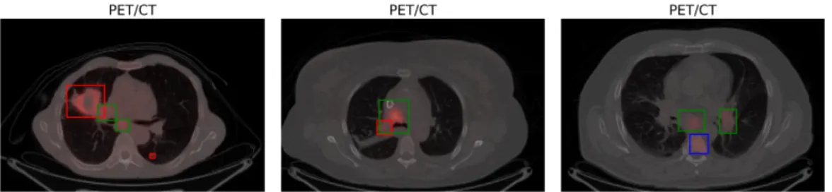
bounding box in red. (Right) PET/CT image for the same region. There is a distinctive glare in the region for the corresponding tumorous region. . . 14 3.2 PET/CT image with malignant tumorous regions bounded by bounding boxes. Primary tumors
are bound by red bounding boxes, nodular tumors by green bounding boxes, and metastasis tu- mors are bound by blue bounding boxes. Note that nodular tumors can appear in close proximity to primary tumors. They often merge with one another making the task of distinguishing them apart difficult. On a similar note, nodular and metastasis tumor can appear in close proximity with one another. . . 15
Each of the green blocks is a ResNet block that consists of two consecutive sub-blocks. Each such sub-block consists of Group Normalization, ReLU, and Convolutional layers stacked one after another. The attention gates filter the skip connections before being added to the downstream layers. The output of the model (colored in blue) is a single channeled probability map of the tumorous region with the same spatial resolution as the input CT image. The details of the attention gate are shown in Figure 4.2. . . 20 4.2 The Figure shows a schematic representation of the proposed PET Guided Attention Gate. The
input feature representationxlis scaled by attention maskα, which is computed by the attention gate. Spatial and contextual information are captured by two gating signals: the encoded feature representationgand the composite functionh(x). The composite function is zero when the PET images are missing and the output of the functionf(xP ET) when PET images are available. PET image representation and not the PET image itself is fed to the attention gate. . . 21 4.3 The significance of the dice coefficient can be understood from the schematic diagram shown in
this Figure. Let the circle shaded in blue be the space of ground truth segmentation masks.
Correspondingly, let the other circle shaded in red be the space of predicted segmentation masks.
Then the dice coefficient is an intersection of the two shaded circles discounted by the sum of the cardinalities of the individual circles. Adapted from [36] . . . 27 5.1 The Figure shows the performance of the baseline models and the PAG model on validation and
test datasets (metrics: dice coefficient, precision and recall). PAG:ct and PAG:ct+pet are the consequence of one and the same PAG model. PAG:ct+pet is PAG model when PET images are input to the model. Conversely, PAG:ct is PAG model when PET images are not input to the model. PAG:ct performs at par with the unimodal and unimodal+attn models. Similarly PAG:ct+pet model performs at par with the bimodal and bimodal+attn models. However, some aberrations to the pattern can be observed. These aberrations could be due to the variation in the dataset. . . 32 5.2 The Figure shows the performance of the baseline models and the PAG model on validation and
test datasets when categorized according to the type of tumor. Again, PAG:ct model performs at par with unimodal and unimodal+attn models while PAG:ct+pet model performs at par with bimodal and bimodal+attn models. Once again the observed aberrations could be due to the variation in the dataset. . . 33 5.3 The Figure shows the dice coefficient for the PAG model and the bimodal model when the fraction
of total PET images that are made available for training the models is restricted. The red band is the mean and standard deviation of the bimodal model in the limit of complete set of PET/CT images. Similarly, the green band is the mean and standard deviation of the unimodal model trained on complete set of CT images. The degradation in performance of bimodal model is much more drastic than the PAG:ct+pet model. Note that PAG:ct+pet model should always maintain the edge over unimodal model because either of the models were trained on the same number of CT images. However, PAG:ct+pet was also trained on few of the PET images. . . 35
5.4 The Figure shows the three attention masks (alpha-1, alpha-2, alpha-3) of PAG:ct model at three intermediate spatial resolutions of encoder/decoder branches. alpha-1 is the attention mask of the attention gate at the deepest layer, while alpha-3 is the attention mask of the attention gate at the shallowest layer. alpha-2 is the attention mask of the remaining attention gate. The Figure also shows the input CT image, the ground truth, and the predicted segmentation masks.
Nodular tumors are marked in green and the metastasis tumor are marked in blue in the PET/CT image. Note that there is little to no attention for the metastasis tumor although it shows up in the PET/CT image. . . 36 5.5 The attention masks (alpha-1, alpha-2, alpha-3) of PAG:ct+pet model at three intermediate
spatial resolutions of encoder/decoder branches. alpha-1 is the attention mask of the attention gate at the deepest layer, while alpha-3 is the attention mask of the attention gate at the shallowest layer. alpha-2 is the attention mask of the remaining attention gate. The Figure also shows the input CT image, the ground truth, and the predicted segmentation masks. This Figure also shows the same axial slice that is shown in Figure 5.4. Nodular tumors are marked in green and the metastasis tumor are marked in blue in the PET/CT image. Note that there is a strong attention in for the metastasis and the nearby nodular tumor. This could be due to the addition of PET image which helps in learning informative attention masks. . . 37 B.1 The Figure shows precision and recall for the PAG model and the bimodal model when the
fraction of total PET images that are made available for training the models is restricted. The red band is the mean and standard deviation of the bimodal model in the limit of complete set of PET/CT images. Similarly, the green band is the mean and standard deviation of the unimodal model trained on complete set of CT images. The degradation in performance of bimodal model is much more drastic than the PAG:ct+pet model. Note that PAG:ct+pet model should always maintain the edge over unimodal model because either of the models were trained on the same number of CT images. However, PAG:ct+pet was also trained on available PET images. . . 48 B.2 The Figure shows the sensitivity (or recall) of segmentation of primary and nodular tumors for
the PAG model and the bimodal model, when the fraction of total PET images that are made available for training the models is restricted. The red band is the mean and standard deviation of the bimodal model in the limit of complete set of PET/CT images. Similarly, the green band is the mean and standard deviation of the unimodal model trained on complete set of CT images.
The degradation in performance of bimodal model is much more drastic than the PAG:ct+pet model. It is expected that PAG:ct+pet should always maintain the edge over bimodal model.
While, this trend can be observed for the primary tumors, it cannot be observed for nodular tumors. The performance of both the models is comparable with one another. . . 49 B.3 The Figure shows the sensitivity of segmentation of metastases tumors for the PAG model and
the bimodal model, when the fraction of total PET images that are made available for training the models is restricted. The red band is the mean and standard deviation of the bimodal model in the limit of complete set of PET/CT images. Similarly, the green band is the mean and standard deviation of the unimodal model trained on complete set of CT images. The degradation in performance of bimodal model is much more drastic than the PAG:ct+pet model. It is expected that PAG:ct+pet should always maintain the edge over bimodal model. However, an opposite trend is observed here. This trend is quite counter-intuitive but is plausible because of the variation in the current dataset. Also, recall shows high variance when the size of segments is small which could be another reason for this trend. . . 50 B.4 The Figure shows the three attention masks (alpha-1, alpha-2, alpha-3) of PAG:ct and PAG:ct+pet
models at three intermediate spatial resolutions of encoder/decoder branches. alpha-1 is the at- tention mask of the attention gate at the deepest layer, while alpha-3 is the attention mask of the attention gate at the shallowest layer. alpha-2 is the attention mask of the remaining attention gate. The Figure also shows the input PET/CT image, the ground truth, and the predicted seg- mentation masks. Nodular tumors are marked in green and the metastasis tumor are marked in blue in the PET/CT image. The attention masks of PAG:ct+pet model show a strong attention in the metastasis and nodular tumors unlike the attention masks of PAG:ct model. The stronger attention can be attributed to the input PET images. . . 51
4.1 The Table shows the layers of the encoder. The ResNet block is a series of two sub-blocks stacked one after another. Each of the sub-blocks consists of GroupNorm layer, ReLU layer and a Convolutional layer. A schematic representation of the ResNet block is shown in Figure 4.1 . . 23 4.2 The Table shows the layers of the decoder. UpLinear represents 3D bilinear interpolation and
AddId represents an addition of filtered skip connection. The definition of ResNet block is analogous to the one defined in Table 4.1 . . . 23 4.3 The Table shows the layers of the functionf(xpet). The functions extracts features from the PET
images. These extracted features are input to the attention gate. The definition of ResNet block is analogous to the one defined in Table 4.1. . . 24 5.1 Hyper-parameters set across all the models. (pparameter appropriate for PAG model only.) The
hyper-parameters were set based on the performance on one of the folds at a different seed than that is used for evaluation of models. . . 31 A.1 Definitions for the Primary, nodular and metastases tumors stage classifications according to
TNM staging protocol. Definitions adapted from [Edge B.S., 2010, p 257-263]. . . 45 A.2 Labels for the locations of the nodular tumors defined according to TNM staging protocol. Def-
initions adapted from [Edge B.S.,2010, p 257-263]. . . 46 A.3 The T-labels, N-labels ad M-labels that are present in the current dataset. The T-labels are
for the primary tumors, the N-labels are for the nodular tumors and the M-Labels are for the Metastasis tumors. They are defined by their respective stages and locations according to TNM staging protocol. The T-label stage is the one that primarily decides the stage of cancer. . . 46
Lung cancer, like any other form of cancer, is usually diagnosed by a combination of several clinical tests such as imaging, sputum cytology, and biopsy tests. Among such tests, computed tomography scanning (CT scanning) is a widely used medical imaging procedure for the diagnosis of lung cancer. More recently, positron- emission tomography scanning (PET scanning) is done in conjunction with CT scanning for a more extensive and rigorous staging of cancer. While a CT scan can provide anatomical and structural information of the tumor, a PET scan provides functional and metabolic information of the tumor. Often PET and CT images are referred to as two distinct modalities as they provide complementary information of the same region of interest. However, the sheer number of lung cancer patients makes the task of distinguishing tumorous from non-tumorous regions in PET/CT images very strenuous and challenging. Recent advances in artificial intelligence have motivated research efforts into developing automated tools for the segmentation of these tumorous regions (known as Computer-Aided Detection and Diagnosis systems or CAD systems) to reduce the onus on the healthcare providers. PET images, in addition to CT images, are an invaluable tool for the automated segmentation of tumorous regions. Nonetheless, it is not always the case that a PET image is readily available for a corresponding CT image, especially in limited-resource settings. This could be due to various technical and practical reasons.
For example, the cost of procuring a PET scan is quite exorbitant. While it costs an average of 2300 USD for a whole-body PET/CT scan, it costs only 230 USD for a CT scan in NYC, USA2. As a result, PET/CT data is often incomplete. It is thus not uncommon to find missing PET images for corresponding CT images in medical databases such as biobanks, which poses a significant challenge in developing such CAD systems.
Conventional models are agnostic to this challenge and make an underlying assumption that a restricted set of modalities (CT or PET/CT data) are always available, which may not be valid. In other words, such models only cater to CT data or PET/CT data, but not both. Prior work in missing modalities has highlighted this challenge, and several other approaches have been proposed to deal with it. Most of the methods attempt to learn effective joint representations of PET/CT modalities. However, such models still assume a complete set of PET/CT data is available during training, to learn such joint representations. Consequently, while such models might be efficient during inference, they fall short in not being able to learn effective joint representations when PET images are missing. The problem is further compounded by the complexity of the data, which could, in principle, encompass a wide tumor-spectrum. This then means that such models might not be capable of making the best use of incomplete PET/CT data.
1https://www.cancer.gov/about-cancer/understanding/statistics
2https://radiologyassist.com/forms/
1.1 Focus of this work
In light of the challenges, as mentioned earlier, in this thesis, we propose a novel deep learning model based on a visual soft attention mechanism. The attention mechanism allows us to input PET images when they are available. As such, the model benefits from the additional modality of PET images but does not mandate them. The model is thus flexible to the availability of PET images. Consequently, two separate models that are trained on unimodal or bimodal data (CT or PET/CT data) respectively are incorporated into one single model. Therefore, in the absence of PET images, the model performs at par with a model that is trained on only unimodal data. Similarly, in the presence of PET images, the very same model performs at par with a model that takes on only bimodal data.
As we noted earlier, one has to make an assumption that a complete set of modalities is available during training in order to learn effective joint representations of PET/CT images. This assumption does not allow us to make the best use of incomplete PET/CT data. In contrast, we do not explicitly enforce the attention mechanism to learn joint representations of PET/CT images. This enables us to use missing PET images during training as well. When the PET images are very scarce in comparison to the number of CT images (i.e., many missing PET images), the model can leverage upon the superfluous CT images for which PET images are missing. In other words, it can be said that the model has the potential to make the best use of incomplete PET/CT data unlike conventional models. We present the effectiveness of the model on an in-house dataset with the goal of segmenting tumorous regions.
In regards, the main contributions of the current thesis are enlisted as follows:
• Propose a novel approach of incorporating missing PET images based on a visual soft attention mechanism.
• Incorporate two discrete functions that deal with unimodal or bimodal data, respectively, under one single model.
• Establish the utility of the model in scenarios when PET images are scarce relative to CT images to show how the model makes efficient utilization of the incomplete PET/CT data.
At the heart of the proposed model is an attention mechanism. At the core of the attention mechanism is an attention gate guided by PET images when available. Hence the model is acronymed as PAG or PET Guided Attention Gate referencing its attention gate.
1.2 Thesis organization
The thesis can be followed in three broad units. We set the context for the whole problem in Chapter 2 and partly motivate why we are doing what we are doing. We then discuss the building blocks of the proposed methodology. Later, we discuss some of the research applications in medical imaging, followed by some specific applications in PET/CT imaging. After that, we discuss how the problem of missing PET images is dealt with in general. As a prelude, we highlighted that prior approaches that deal with missing PET images fall short of being able to learn efficient joint representations of PET/CT modalities. We discuss this problem in detail, followed by a road map to attention mechanisms and how they could potentially circumvent it.
We then proceed further to discuss some of the methodological aspects of the current work. We first introduce PET/CT data in Chapter 3. We then discuss some of the challenges with the current dataset. Complex datasets usually have a high amount of variation in them, which poses a significant challenge to developing CAD systems.
We discuss some of these aspects with the current dataset. Later in the Chapter, we also discuss some of the data pre-processing strategies. After that, in Chapter 4, we discuss the proposed methodology in great detail.
We then discuss some of the implementation details, such as training strategy, choice of loss functions, and evaluation metrics.
Finally, in Chapter 5, we present experimental techniques we used to evaluate our approach. We first validate the performance of our model in comparison to baseline approaches. Later, we present the results of an ablation framework that concretely demonstrates the contributions of the model. Besides, we also present the role of the attention mechanism. We then conclude the thesis with a discussion of the limitations of the current methodology, its practical utility, and opportunities for future work.
and the backbone of the proposed PAG model. Finally, we review some of the prior work in Section 2.3. We also re-iterate the significance of the current work in this Section. We finally summarize the Chapter by including some takeaway concepts/messages.
2.1 What is lung cancer and how is it diagnosed?
2.1.1 Lung Cancer
Lung cancer is a type of cancer that starts in the lungs. There are two types of lung cancer: non-small cell lung carcinoma (NSCLC) and small cell lung carcinoma (SCLC). They are grouped as such according to the type of diagnosis, treatment strategies, and prognosis. NSCLC accounts for at least 80-85% of lung cancer diagnoses, while SCLC accounts for the rest. SCLC tends to grow and spread more rapidly than NSCLC. It will have usually started to metastasize by the time it is diagnosed for most of the patients. While this type of lung cancer is more responsive to chemotherapy and radiotherapy, it has greater potential to relapse.
Regardless of the type of lung cancer, it is the second most commonly diagnosed cancer both in men and women only after prostate cancer in men and breast cancer in women. For example, it is estimated that 116,300 men and 112,520 women shall be diagnosed with lung cancer in the year 2020. Likewise, it is estimated that about 72500 men and 63220 women will, unfortunately, lose their lives to lung cancer in the same year. Further, lung cancer makes up to 25% of all cancer-related deaths, and the number of people that die from lung cancer is more than that of breast, prostate, and colon cancers combined. These statistics [31] underscore how notorious is lung cancer and how important it is to develop early diagnosis tools and methods.
Lung cancer detection and diagnosis
Lung cancer is diagnosed by a combination of imaging procedures and biopsies. While the imaging procedures are non-invasive, the biopsy methods are invasive. Commonly used imaging procedures are X-ray scanning, computed tomography (CT) scanning, and positron emission tomography scanning (PET). These scans are performed to get a clear picture of the suspicious regions that might be cancerous. However, invasive procedures such as biopsies are always performed to confirm the diagnosis. Typical procedures include sputum cytology, thoracentesis, or a simple needle biopsy. In sputum cytology, for example, a sample of sputum is analyzed for the presence of cancerous cells, whereas in a needle biopsy, cells extracted from suspicious areas are analyzed whether or not they are cancerous.
Once the diagnosis has been confirmed by the doctor, a staging of the cancer is performed that stratifies the aggressiveness of cancer. Lung cancer manifests in four stages. It is based on how much cancer has spread to nearby lymph nodes, extraneous regions of the lungs, and regions distant from the lungs, such as the liver.
Lung cancer is staged according to the type of lung cancer i.e., NSCLC or SCLC. NSCLC is staged according to the following criteria.
Stage I: The cancer is located only within the lungs only and has not yet started to spread.
Stage II: The cancer has started to spread to nearby lymph nodes at proximity to the origin of cancer but is within the lungs only.
Stage III: The cancer is spread across the lungs and the lymph nodes in the middle of the chest but is still found within the lungs only.
Stage IV: This is the most advanced stage of cancer when it has started to metastasize, thereby spreading to both the extraneous lung regions, nearby fluid regions and regions distant away from lungs such as the chest, liver or colon.
On the other hand, SCLC is staged as either limited or extensive, depending on whether the cancer has started to metastasize or not.
2.1.2 PET/CT imaging
CT imaging is a non-invasive technique that reconstructs a volumetric description of the region of interest from a combination of X-rays taken from different angles around it. CT produces data that can be manipulated to reveal different bodily structures based upon their degree of absorption of X-rays. Bone tissues, for example have a greater absorption capacity than lungs. This degree of absorption is given by what is known as attenuation coefficients. However, a more common unit of measure is Hounsfield units (HU) which is a linear transformation of attenuation coefficients such that water and air at standard temperature and pressure conditions (STP) have 0 and -1000 HU respectively. HU calculated in terms of attenuation coefficients is given by Equation 2.1 where µis the attenuation coefficient. Raw CT data is usually expressed in terms of these Hounsfield units (HU).
HU = 1000× µ−µwater
µwater−µair
(2.1) On the other hand, PET imaging is gaining traction for its ability to distinguish tumorous from non-tumorous regions apart. It is a type of imaging technique that detects the relative uptake of radioactive materials by tissues called radiotracers. The commonly used radioactive tracer used for lung cancer diagnosis is 18F-FDG molecule, which is a particular type of glucose molecule. Since tumorous regions show greater metabolic activity than non-tumorous ones, they actively absorb the glucose molecule at higher rates. Apart from these tumorous regions, it is also actively absorbed in other regions of active metabolism, such as the brain or the kidneys. The units of measure in a PET scan is Bq/ml (Becquerel per ml) that is indicative of the radioactive concentration.
Accordingly, a PET scan can be thought of as a heatmap of the metabolic activity of the region of interest.
PET/CT scanning is an emerging technology where the PET images are superimposed on CT images, which are obtained from the same scanner simultaneously. Thus complementary information from two different modalities is fused into one another. However, PET/CT scanning is relatively new, and it has some of the most advanced and complicated technologies. Further, it is at least a couple of times more expensive than conventional CT scanning. These challenges inhibit the wide-spread adoption of PET/CT scanning, especially in resource-limited settings. Consequently, it can be safely claimed that the cardinality of the total available CT images is at least a couple of times more than the cardinality of the total available PET images. It is thus not uncommon in clinical databases to have only CT images for which PET images are missing. This poses a serious challenge in making efficient use of incomplete PET/CT data in order to develop robust CAD systems.
We shall see how we deal with this problem in the upcoming discussions.
2.2 Background methods
This section sets the stage for a formal discussion of the proposed PAG model. As a quick reminder, the focus of the current work is to account for the missing PET images for the segmentation of tumorous regions.
Segmentation of objects in an image is a well-studied problem in computer vision. By segmentation, we are primarily interested in assigning a label to every pixel within an image such that pixels with the same label represent the same object in the image. Each unique object of interest in an image is usually assigned a unique class label. Consequently, it is not uncommon to find multi-label (called as multi-class, each class representing each of the unique labels) segmentation tasks.
In this work, we deal with the segmentation of tumors disregarding the variation that exists in tumor shapes, morphologies, etc. We motivate our design choice in the upcoming discussions. However, it suffices here to say that we label each pixel belonging to a tumorous region as one (or foreground), and each pixel belonging to
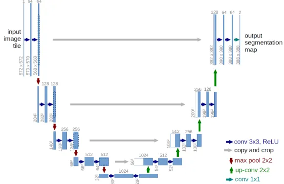
Figure 2.1: A U-Net architecture that consists of contracting, bottleneck, and expanding sections resembling a U-shaped structure. The contracting and the bottleneck sections are referred colloquially as an encoder and the expansion section as a decoder. The encoder learns rich high dimensional feature representations while the decoder decodes the feature representations for the problem at hand. Adapted from [27]
a non-tumorous region as zero (or background). We accomplish this not by directly labeling each foreground or background pixel as one or zero. We rather predict a probability for each pixel belonging to foreground or background. Any pixel that has a probability value higher than a user-defined threshold is labeled as foreground (or as a tumorous region). The inverse applies to a non-tumorous region. We are then primarily interested in predicting a probability map of tumorous regions given the input data. This probability map can be appropriately thresholded to yield the desired segmentation.
The proposed PAG model is tailored to get such a probability map of the tumorous regions given the PET/CT images that account for the missing PET images. It is built upon standard U-Net architecture [27], ResNet blocks [15], and a visual soft attention mechanism. In order to understand the proposed PAG model, it is worthwhile to go through some of these concepts, which is the focus of the current section.
2.2.1 U-Net
One of the main building blocks of the proposed PAG model is a U-Net architecture. It is one of the most versatile deep learning architectures for image segmentation. For a binary image segmentation problem, a U- Net yields a probability map of the same spatial resolution as the input image. This probability map is then thresholded to get the desired segmentation map. The architecture was initially proposed for biomedical images, which has then been widely adopted for other image segmentation tasks.
U-Net is a fully convolutional neural network (FCN), meaning which it does not have any fully connected layers. It consists of encoder and decoder structures just like a conventional FCN architecture but with the addition of skip connections resembling that of a U shape and hence its name. As shown in Figure 2.1, U-Net consists of three prime sections: a contracting section, a bottleneck section, and an expansion section, respectively. The contracting section is a series of convolutional layers followed by non-linear activations (usually ReLU activations) and max-pool layers. The convolutional layers, along with non-linear activations, learn high dimensional non-linear features while the max-pool layers downsample the spatial resolution of the image. A bottleneck layer follows the contracting section. It consists of convolutional layers and non-linear activations to extract a rich high dimensional representations of the input image tailored for the specific task of concern. The contracting section, along with the bottleneck section, is colloquially referred to as an encoder as it encodes the input in a higher-dimensional space. Typically for image classification tasks, a fully connected layer follows this encoder to get a probability of the image belonging to a particular class. However, for image segmentation tasks, what we need is a probability map of each pixel belonging to either foreground or background. The
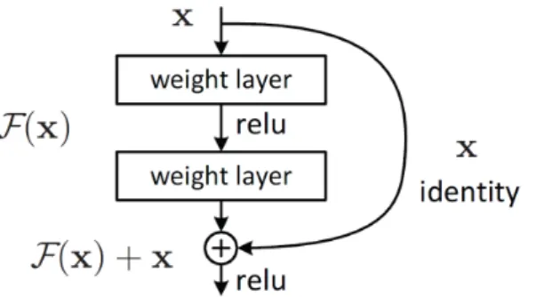
Figure 2.2: The Figure shows a ResNet block that consists of one identity layer and two weighted layers. The identity layer is added to the network two layers downstream. Skip connections such as these help in tackling the problem of vanishing gradients. Adapted from [15
expansion section achieves this. The encoded feature representation is upsampled by a series of deconvolutional operations (upsampling operations that increase spatial resolution), convolutional layers, non-linear activations, and skip connections. The output of the expansion section is a probability map with usually the same spatial resolution as that of the input image. The expansion section is colloquially referred to as a decoder as it decodes the encoded feature representation.
One of the unique features of a U-Net that makes it stand apart from a conventional FCN are the skip connections. The feature representations extracted from the initial layers of the contracting section are concate- nated directly to the layers of the expansion section, which is what we call as skip connections because we are skipping some intermediate layers in the process. These skip connections provide necessary information to the expansion section of the U-Net that could have been lost during the contracting section. They also help tackle the problem of vanishing gradients. Deep neural networks can suffer from vanishing gradients when gradients have to flow through multiple layers. Skip connections help avoid this problem because they pass the gradient information to the lower layers without discounting them through the intermediate layers.
2.2.2 ResNet
The second building block of the proposed PAG model is a ResNet block. The motivation for ResNets can be understood as follows. One of the breakthroughs in deep learning occurred with the introduction of AlexNet neural network architecture [19] when it achieved a top-5 error rate of 15.3 %, more than 10.8% lower than the runner up in ImageNet 2012 challenge [28]. The success of AlexNet was attributed to the depth of the model architecture. It has nearly 62M (62 million) parameters. Consequently, it was believed that deeper neural networks tend to perform better than their shallower counterparts. Hence, the trend back then was to make neural networks deeper and deeper. Some noteworthy contributions include VGG neural network [30], which has close to 138M parameters. However, it was observed that making networks deeper was becoming counter- productive. This problem was attributed to the fact that very deep neural networks suffer from the problem of vanishing gradients. Consequently, architectures with residual blocks or ResNets [15] were introduced to tackle this problem of vanishing gradients. While there were other approaches that address this problem [34], the breakthrough happened with the introduction of ResNets.
At its core, ResNet is an idea of adding an identity layer after a few layers downstream. As shown in Figure 2.2, there is an identity layer after two weighted layers. The weighted layers map the input to an output say F(x). The final output of the ResNet block is F(x) +x, which is akin to stacking an input layer to its output. The authors claim that their approach of stacking layers should not degrade the network performance because we could stack identity mappings on the current network (a layer that does not learn anything). The resulting architecture should perform the same. The authors hypothesize that letting stacked layers fit in this way is easier than letting them directly fit the underlying mapping because of faster convergence. The gradients can now flow from later layers to earlier layers without vanishing or being discounted by intermediate layers, therefore, alleviating the problem of vanishing gradients.
2.2.3 Visual Attention
The English meaning of attention is to take note of someone or something exciting or important. Similarly, in machine learning, attention mechanism means a group of techniques that help a model attend to the most critical and discriminatory parts of an image.
There are two broad categories of visual attention mechanisms: hard attention and soft attention. Hard
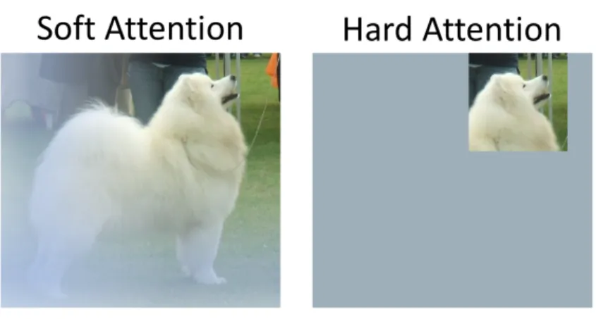
Figure 2.3: The Figure compares the result of applying soft attention and hard attention masks to the input image. While soft attention uses attention masks with values in the range [0,1], hard attention uses attention masks that strictly take on a value of either one or zero i.e.,{0,1}. Consequently, soft attention masks amplify critical sub-regions of the images and suppress irrelevant sub-regions of the image. While hard attention masks simply crop the critical sub-regions of the image. Adapted from [8]
attention uses image cropping to focus upon regions of interest. Models based upon hard attention can however, not be trained using gradient descent algorithms, as such models are inherently built upon sampling cropped image regions. They are trained using policy gradient methods (for ex. REINFORCE), a subclass of Rein- forcement learning algorithms. On the other hand, models based upon soft attention mechanisms try to learn a probability map that amplifies relevant discriminatory regions and suppress irrelevant regions. Such models can be trained using standard gradient descent algorithms such as backpropagation. The distinction between soft attention and hard attention is self-evident, considering Figure 2.3.
In its simplest form, let x ∈ Rd be an input vector, a ∈ [0,1]k be attention coefficients obtained by an attention networkfφ(x) with parametersφ,z∈Rk be a feature vector that is obtained by a non-linear function fθ(x) with parameters θthen
a=fφ(x) (2.2)
z=fθ(x) (2.3)
y=az (2.4)
whereis an element wise multiplication andy∈Rk is the result of the attention mechanism where irrelevant features have been pruned and important features amplified. In soft attention, the mask ais allowed to have values in the range [0,1] whereas in hard attention, the mask is allowed to have only one or zero values i.e.
a∈ {0,1}k. Therefore, attention mechanisms help compute masks which can be used to select essential sub- features and discard non-essential ones.
The heart of the proposed PAG model is a visual soft attention mechanism first introduced by Jetley et al.
[2018] for image classification. Before going any further, it is essential to understand the intuition behind such an attention mechanism, which can be reasoned as follows.
Attention mechanism: Intuition
For an image classification task, the encoded feature representationgextracted at the penultimate layer from a CNN architecture expresses an image in a high dimensional space in which different dimensions represent salient higher-order visual concepts, to render different classes linearly separable. It can be argued that allowing an intermediate feature representation earlier in the networkxl at layerl to learn mappings, compatible with the encoded feature representationg would help in boosting the performance of a model. This can be achieved by allowingxl to contribute to the final classification step only in proportion to its compatibility withg. In other words, the compatibility score is high if and only ifxl has dominant discriminatory features for the particular class of concern. Likewise, feature representations at intermediate spatial resolutions can be similarly enforced to be compatible withg. This allows different class level features to be extracted at different spatial resolutions. In other words, it is proposed to use an attention mechanism that allows feature representations at different spatial resolutions to be guided by an encoded feature representationg in order to attend to the most discriminatory
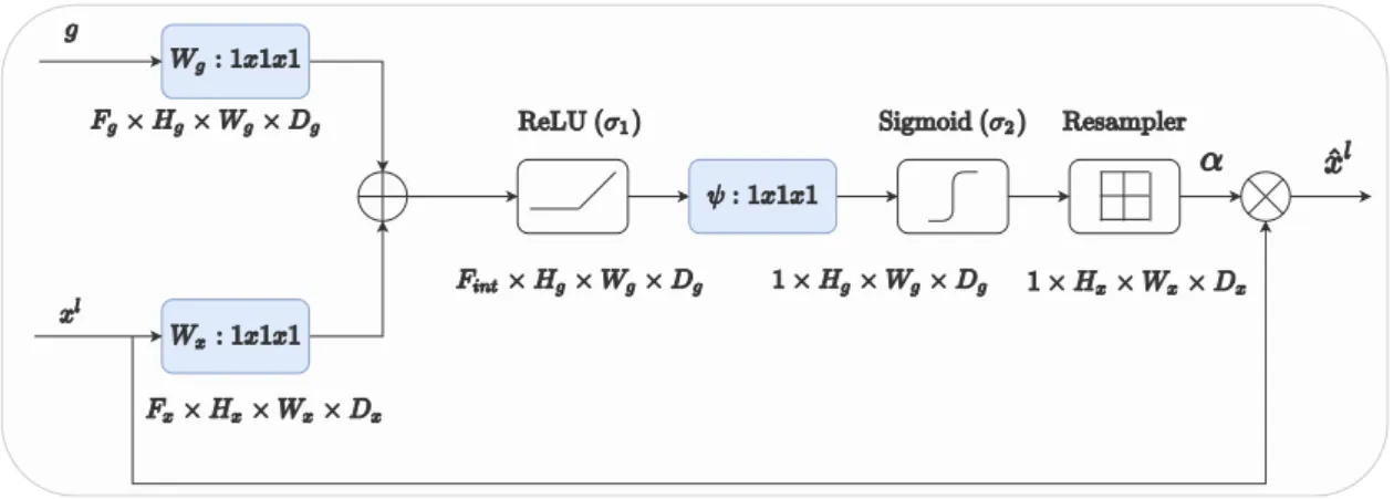
Figure 2.4: The Figure shows an attention gate. It filters the input feature representation xl by attention coefficientsα, which are learned by the attention gate. The gating signalg provides context to the attention gate.
features. Note that this encoded feature representationgis known by different names as context vector, guiding signal, or a query signal. These words are used interchangeably, depending on the context. However, the takeaway message is that the encoded feature representation g provides context for learning salient attention masks that prune irrelevant sub-features and amplify, important sub-features of the feature representation.
Attention mechanism: Attention gate
Oktay et al.[2018] build upon the afore-discussed reasoning and propose an attention gate for pancreas segmen- tation. It can be easily plugged into any U-Net type architecture for image segmentation. It takes two inputs as shown in Figure 2.4: (a) the encoded feature representation g and (b) the intermediate feature representation xlafter layerl(output of the encoder at a particular spatial resolution).
xlis obtained by applying a linear transformation (convolutional operation) followed by a non-linear activa- tion function (usually ReLU activation) to the output of preceding layerl−1 i.e. xl−1. xlcontains rich higher dimensional representation of the input image. Accordingly, ifFl is the number of feature channels ofxl then xlc=σ(P
c0∈Flxl−1c0 ∗kc0,c) where∗denotes the convolution operation. kc0,care the filter weights of appropriate dimensions and σ denotes a suitable activation function. The attention gate is trained to learn the attention coefficientsαi ∈[0,1] for each pixelithat identify salient features that are discriminatory for the specific task of concern. The output of the attention gate is the element wise multiplication of the input feature representation and the computed attention coefficients: ˆxli,c =xi,c·αli for channel c and pixel ifor the given layer l. (Note that xli ∈RFl & ˆxli ∈RFl). The output of the attention gate can thus be thought of being the result of input feature representation being scaled by the attention coefficients where important discriminatory regions of the feature representation are amplified and irrelevant regions suppressed.
More concretely, let g represent a context vector with Hg×Wg×Dg spatial resolution and Fg number of channels respectively. Similarly letxl represent a feature map with Hx×Wx×Dx spatial resolution and Fl number of channels respectively. Then for each pixel i, the pixel vector is given as xli ∈ RFl and the gating vector is given asgi ∈RFg. Then, the attention coefficients are given by the following Equation
qattl =ψT(σ1(θTxxli+θgTgil+bg)) +bψ (2.5) αli=σ2(qattl (xli, gi; Θatt)) (2.6) whereσ1(x) andσ2(x) correspond to ReLU and sigmoid activations respectively. The parameters of attention gate Θattare given byθx∈RFl×Fint,θg∈RFg×Fint,ψ∈RFint×1and bias termsbψ ∈R,bg∈RFint. The linear transformations are computed using channel-wise 1×1×1 convolutional operation for the input tensors.
Attention mechanism: Attention U-Net
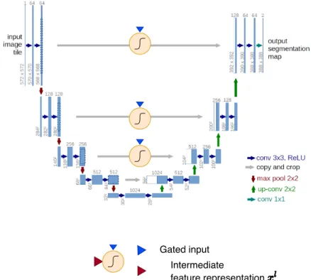
The attention gate, as discussed earlier, is the main component of the attention mechanism. The gate can be plugged into a standard U-Net architecture, as shown in Figure 2.5. It can be seen that there are three attention gates with each of the attention gates learning distinct attention coefficients for intermediate feature representations at three different spatial resolutions of the encoder block. While the attention gate appears only in the decoder block and not in encoder block, it can be inferred that it helps in better decoding the encoded
Gated input Intermediate
feature representation
Figure 2.5: The Figure shows an Attention U-Net. The architecture is similar to a U-Net architecture except with the addition of three attention gates for each of the skip connections at three intermediate spatial resolutions.
The attention gates filter their skip connections before being concatenated. Adapted and modified from [27]
feature representation. The performance improvement can then be attributed to the smart way of decoding the encoded feature representation.
2.3 Related work
2.3.1 A roadmap to PET/CT images in deep learning
Segmentation of anatomical structures such as tumors, brain lesions, or lung nodules from medical images is an active and dynamic area of research within medical imaging. A multitude of automated tumor segmentation methods has been proposed over the last two decades. Some of the earlier contributions include that ofGeremia et al. [2011] on the detection of white-matter multiple-sclerosis (MS) lesions of the brain. They manually extracted local and context-aware intensity-based features for training a random decision forest algorithm for the classification of individual voxels into malignant and non-malignant lesions. Motivated by the success of Random Forest models in the BRATS 2012 challenge,Tustison et al.[2013] extracted tissue-specific probability priors using generative Gaussian Mixture models and then implemented Markov Random Fields (MRF) to learn their MAP estimates. MRF was also used as a spatial regularizer to enforce spatial continuity.
It was long understood that PET/CT dual-modality aids in the detection of tumors thanks to the study byAntoch et al. [2004]. They concluded that PET/CT fusion images are more effective than unimodal PET or CT images for manual detection of tumors. Automated tumor detection systems were developed based on this understanding to extract multi-modal PET/CT features, in contrast, to stand alone unimodal PET or CT features. Consequently, we find thatSong et al. [2013] formulated the tumor segmentation problem as a minimization of MRF that encodes information from both the modalities. The model was subsequently learned through graph-cut algorithm. Further, Guo et al. [2014] used fuzzy MRF (Markov Random Field) to learn a maximum a posteriori for each voxel belonging to a tumorous or non-tumorous region.
Such models are however, limited by the extraction of the domain and task-specific features that often lack sufficient representational capacity. At about the same time, deep artificial neural networks emerged as a promising alternative for their ability to learn highly representative features without the need for any manual feature extraction. Specifically, convolutional neural networks (LeCun et al.[1998];Krizhevsky et al.[2012]) have shown promising results in the field of computer vision and medical imaging which sparked copious amount of research. For example, Akselrod-Ballin et al. [2016] employed a deep learning model for the detection of tumors in breast mammograms. The model consisted of layers of pre-processing steps and a modified Faster
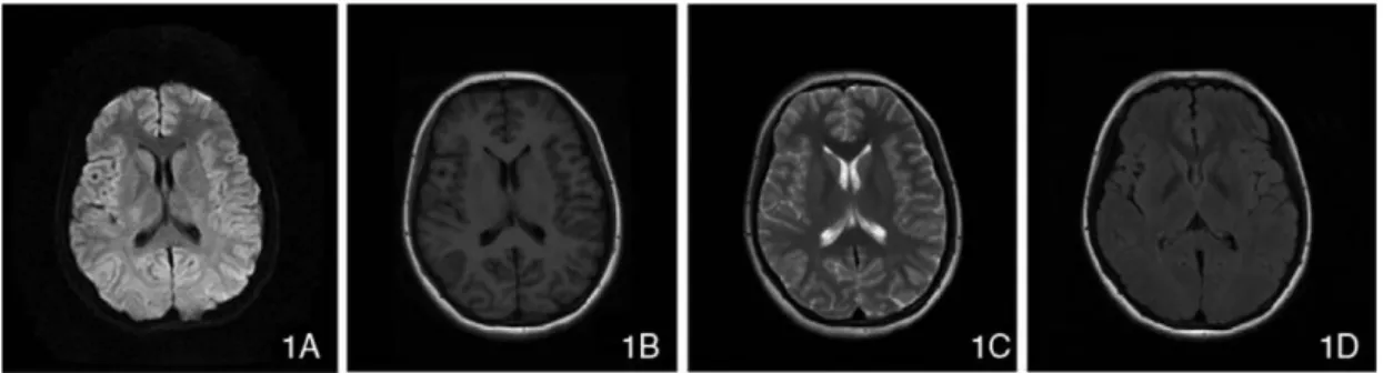
Figure 2.6: Figures 1A-1D represent DWI, T1-weighted, T2-weighted, and FLAIR modalities of MR images.
The respective modalities are well correlated with one another. They only differ in their respective intensity patterns. Adapted from [7]
R-CNN (Ren et al. [2015]). Further, Carneiro et al. [2015] developed a classification system based on a pre- trained deep learning model that gives the risk of a patient developing breast cancer using the Breast Imaging- Reporting and Data System (BI-RADS) score. They trained a CNN classifier on the features extracted from multi-view unregistered input images that predicts the desired BI-RADS score. Xu et al. [2015] extracted high dimensional features using pre-trained deep learning models from large scale brain tumor histopathology images for classification and segmentation of tumors. These are just a few examples among the oceanic applications that popped up after the promise of deep learning.
The domain of PET/CT images is no different. Zhao et al. [2019] implemented a U-Net architecture [27]
for the segmentation of nasopharyngeal tumors from dual-modality PET/CT images. Li et al. [2019] learned a probability map of tumorous regions from a CT image. They then propose a fuzzy variational model that incorporates the probability map as a prior and the PET images to obtain a posterior probability map of tumorous regions. Their method allowed one to fuse the information from PET/CT images in an intelligent manner in contrast to a naive channel concatenation. Guo et al. [2018] studied different fusion schemes of multi-modal images. They studied three fusion schemes: one at the input channel layer, one at the intermediate representation layer, and lastly, at the final classification layer. They found that the fusion of multi-modality images at the intermediate representation layer has the best performance but point out that it is more sensitive to errors in the individual modalities.
2.3.2 How is the problem of missing PET images tackled?
The methods mentioned above are however, either based on unimodal or multi-modal input images. They tacitly assume that a complete set of all the modalities that were used while developing the model is available even during inference. Such methods do not have the capacity to incorporate for missing modalities. Accordingly, several other methods have been proposed that deal with missing modalities. Havaei et al. [2016] proposed the Hemis model to extract representations from multiple MR image modalities (such as DWI, T1-weighted, T2- weighted, FLAIR) and fuse them in a latent space where linear operations such as the first and second moments of the representations can be calculated. This composite representation can then deconvolved accordingly. The authors tested the applicability of their model to MR image segmentation (on MSGC [35] and BRATS 2015 [22]
datasets). They argue that instead of learning combinatorially different functions, each dealing with a specific missing modality, one single model can be learned that deals with all such missing modalities.
Chartsias et al. [2017] proposed a generic multi-input, multi-output model, which is an improvement over the Hemis model [14] that is equivalently robust to missing modalities. The inputs are the individual modalities of a multi-modal image (for example, multi-modal MR images). The model, which is based on correlation networks [6], was proposed to tackle the challenge of learning shared representations from multi-modal images.
Correlation networks [6] learn effective correlations among individual modality-specific representations in a common representation space. Imposing correlations as such aid in learning a shared (or common) representation space.
Figure 2.6 shows how well MR image modalities are correlated with one another. They are correlated in the sense that all the tumorous regions show specific distinctive properties from non-tumorous regions. They only vary in their intensity patterns. Chartsias et al. [2017] exploited this fact of MR images. They explicitly impose correlations among representations extracted from individual modalities by minimizing the Euclidean distance among one another. However, it is essential to note that for the problem at hand, PET/CT modalities are not as well correlated as the MR image modalities are. While the tumorous regions show a distinctive glare from non-tumorous ones in a PET image, it is very much plausible that a similar glare can be observed
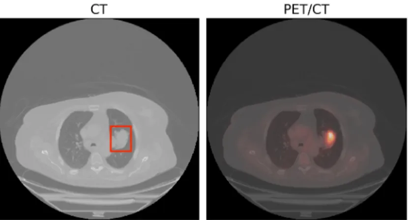
may or may not show up in the PET image depending on their metabolic activity.
in non-tumorous regions as well. Figure 2.7 is an example of such a scenario. It shows a small tumor marked in a red bounding box along with a non-tumorous and active site of metabolism marked in a yellow bounding box. Enforcing correlations as done for MR images may not be the best approach to learn effective correlations among PET and CT representations.
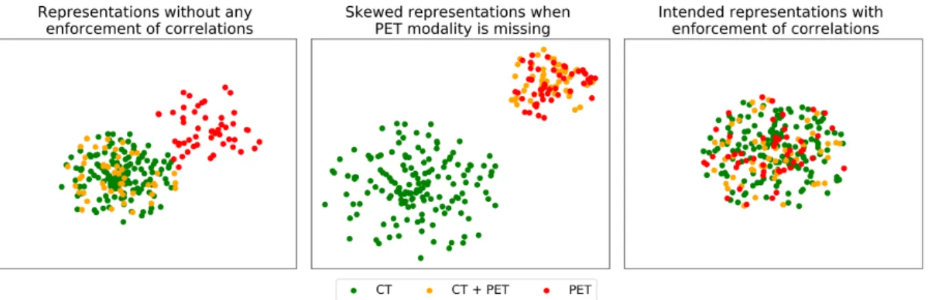
Another drawback of such an approach is that it assumes a complete availability of the respective modalities (PET/CT images for our case) while training the model. Consider that the network is trained on a set of PET/CT images and on a set of CT images for which corresponding PET images are missing. Not enforcing any correlations among the PET and CT representations would give rise to something shown in Figure 2.8 (a). Two distinct clusters can be noticed: one for CT and one for PET image representations, respectively.
Enforcement of correlations among the individual representations should ideally be something as shown in Figure 2.8 (c). Only one distinct cluster is formed for the PET/CT representations. However, when PET images are missing enforcing correlations among respective modalities would result in something shown in Figure 2.8 (b).
This can be understood as follows. When the network is trained on a batch of CT images for which PET images are missing, it does not make sense to enforce correlations as such. Now consider that the network is trained on a batch of PET/CT images. Now correlations among PET and CT representations can be enforced as such.
This then means that the CT representations are pulled towards PET representations unlike in the former case (when training on a batch of CT images for which PET images are missing). This skews the representations to two distinct clusters, as shown in Figure 2.8 (b). Accordingly, two clusters are formed: one for PET/CT images and one for CT images. This skewed representation is not the ideal and intended representation. This problem is further accentuated when there are multiple types of tumors. In the ideal scenario, as many clusters as the different types of tumors are formed, with each cluster having respective PET/CT latent representations clustered among one another (like in Figure 2.8 (c) but as many clusters as for different types of tumors). The complexity increases further, with an increase in the number of modalities.
The Hemis model [14] does not explicitly enforce a correlation among modality-specific latent representations, as explained earlier. It however, does project them into a shared (or common) representation that is effectively a concatenation of mean and variance across the individual representations. The authors argue that when the complete set of PET/CT images is available during inference, the expected variance is supposed to be low in contrast to when the complete set of PET/CT images is not available during inference. However, the calculation of variance across representations enforces a correlation among them indirectly. Consequently, this model should similarly suffer from skewed representations, as noted earlier. We note a similar problem for other approaches that use a similar approach to learning shared representations. We only argue that such approaches are agnostic to the fact that PET images can be missing even during the very development of the model i.e., while training the model. This implies that such approaches are not yet capable of efficiently using the available PET/CT and CT data for learning robust representations.
In light of the aforementioned limitations, we make use of an attention mechanism that does not have to fuse the latent multi-modal representations. We thus, do not enforce any correlations among individual representations. Correlations, if any, are supposed to be learned by the model itself. We argue that it is still possible to retain a robust performance owing to the attention mechanism when salient and discriminatory regions are amplified. In what follows, we take a detour to discuss prior work on attention mechanisms and motivate how this led us to the current work.
Figure 2.8: (a) PET and CT representations when no explicit correlations are enforced while training a model.
(b) Skewed representations when explicit correlations are enforced among PET and CT representations when PET images are missing. PET/CT and CT representations form two distinct clusters. (c) An ideal clustering of PET/CT representations when explicit correlations between PET and CT modalities are enforced even when PET images are missing.
2.3.3 Attention mechanisms: Attend to salient features!
Attention mechanisms in the context of deep learning are inspired by visual attention, which has been primarily studied in neuroscience and computational neuroscience [17]. Humans and animals tend to focus specific regions of an image in ”high resolution” while focusing on neighboring regions in ”low resolution,” thereby adjusting their focal point of view over time. In effect, this means that certain regions are given more importance or attended to over other regions. However, much of the success of attention mechanisms in deep learning was fuelled by advances in Natural language processing (NLP) or, more specifically, Neural Machine Translation (NMT).
NMT aims to translate a sentence from one language to another. With advances in Recurrent neural net- works (RNNs) and Long-short term memory (LSTMs) [16], applications involving NMT have become popular.
However, one of the critical problems of RNNs and LSTMs is that while in theory, they should be able to learn long-range dependencies in the input sentences; in practice, they fail to do so. Irrespective of the length of the input sentences, these models squash them to a hidden representation of a fixed-sized vector by an encoder. The hidden representation gives the context to the decoder to generate the outputs, the translated sentence. Squashing the input sentence to a fixed-sized hidden representation means that cues that appear sev- eral words/sentences before the current word are easily forgotten/discarded. Bahdanau et al.[2014] introduced an attention mechanism that calculates a context vector for each step of the decoder network. The context vector is calculated by using the hidden representations at all the intermediate steps of an encoder network along with the current step of the decoder network. They argue that such a mechanism would reduce the onus on the decoder to decode a highly abstract representation. The decoder now has access to all the intermedi- ate steps of the encoder. The necessary details of how this is achieved are beyond the scope of the current discussion. However, what is important to note is that by letting the decoder access the intermediate steps of the encoder through an attention mechanism, significant performance gains were achieved. While these models still sequentially process their inputs, transformer networks proposed byVaswani et al. [2017] are based on a self-attention mechanism and circumvent the need for sequential processing of input sentences. This brought attention mechanisms into mainstream research in NLP.
While attention mechanisms have had significant impacts in NLP, their widespread adoption in Computer Vision still lags. Notable work is that of Xu et al. [2015]. They attempt to describe an image in a couple of words predicted by the model. The model learns suitable attention masks for each of the generated words, as shown in Figure 2.9. Their attention mechanism is, in principle, similar to the one introduced by Bahdanau et al.[2014].
Jetley et al. [2018] proposed an attention mechanism in lines similar to Bahdanau et al. [2014] but for image classification. Oktay et al.[2018] customize the formulation ofJetley et al. [2018] for pancreas image segmentation. They propose a novel attention gate that learns salient attention masks from a guided signal and a feature representation. We discussed in detail the intuition and formulation of these attention gates earlier.
What is important to note is that the guiding signal gives context to the attention gate in order to learn efficient attention masks. Since PET images can be thought of as a heatmap of tumorous regions within a given CT image, we incorporate them into the attention mechanism. PET images, when available, only act to enhance the context of the guiding signal. This formulation allows the input of PET images to be only complementary
an attention mask that given the word, the attention masks focus on appropriate regions of the image. Adapted from [40]
to CT images but not mandatory. Further, since PET images are only part of an attention mechanism, we do not enforce any explicit correlations among representations extracted from PET/CT modalities. This allows us to deal with the problem of skewed representations, as discussed earlier.
Further, the simplicity of our attention mechanism has the advantage of being incorporated into any pre- existing architecture that is trained on only CT images without making any radical changes. The network can be fine-tuned with the new attention mechanism without much computational overhead, with the advantage of the addition of another modality of PET images. This is however, not the case with previous methods. We note that once developed, they have to be restructured to much greater detail and re-trained.
2.4 Summary
We believe we have given sufficient context for the problem of missing PET images in this Chapter. The following points summarize our discussions so far in this Chapter.
• Lung cancer is a highly notorious disease with high mortality rates across the world. It is imperative that we develop early diagnostic tools. PET/CT scanning plays a key role in the diagnosis of lung cancer.
They provide an attractive opportunity to develop automated computer-aided diagnostic systems (or CAD systems). However, since PET images are expensive, it is not uncommon to find missing PET images.
• Segmentation of tumors is a key step in the development of CAD systems. The proposed model is one such diagnostic tool that can cater to missing PET images. It is based on three building blocks: (a) U-Net architecture, (b) ResNet blocks, and (c) attention gates. We review these methods in sufficient detail required to follow the proposed PAG model.
• We also review some of the prior work in the broad field of medical imaging. We then narrow down to some of the applications that have been made possible due to deep learning. We further review how the problem of missing PET images is usually tackled and note that prior approaches (based on fusion of representations) do not learn intended representations when PET images are absent during training the model. We further allude to how the proposed PAG model addresses these issues.
Data
There is an adage well known among the machine learning community ”Garbage in and garbage out.” Machine learning models are only as successful as the quality of data they are trained upon. It is, therefore, imperative to have a firm understanding of the dataset we shall be dealing with in order to construct efficient data pre- processing strategies. This Chapter introduces the dataset, describes the challenges involved in dealing with it, and then the steps involved in the data pre-processing pipeline.
The dataset consists of whole-body PET/CT scans of 397 lung cancer patients with ICD-10 diagnosis code C34 with histologically proven NSCLC [29]. The scans were obtained between Jan 2008 to Dec 2016 from University Hospital Basel, Switzerland. The patient population consisted of 28% females and 72% males with ages between 38-97 years (71±10.5 years). PET/CT examinations were performed on an integrated PET/CT system (Discovery STE, GE Healthcare, Chalfont St Giles, UK) with 16-slice CT from Jan 2008 to Dec 2016 and on a PET/CT with 128-slice CT (Biograph mCT-X RT Pro Edition, Siemens Healthineers, Erlangen, Germany) from Dec 2015 to Dec 2016. Annotation and volumetric image segmentation of each lesion on transversal slices was performed in random order by a dual-board-certified radiologist and nuclear medicine physician with 9 years of professional experience in PET/CT reading as well as a supervised radiology resident with 2 years of professional experience.
PET/CT images provide complementary information on the regions of interest. PET images can be thought of as a heatmap for the corresponding CT images where the tumorous regions show a marked contrast or a distinctive glare between their surroundings. An example of such a pair of CT images and a PET/CT image (PET image superimposed on CT image) is shown in Figure 3.1. Note that the tumorous region, which is bound by a red bounding box in the CT image, has a marked contrast over its surroundings in the PET/CT image.
This is because of the greater 18F-FDG uptake by the malignant tumors due to higher metabolic activity, which can be detected from PET images. The role of PET images is clear from this Figure as to how a doctor tends to go back and forth between the CT and PET images in order to attend to malignant tumors. The doctor would first scan for the malignant regions in CT images and then affirms his findings from the PET images.
And then, he would scan for suspicious regions in the PET images only to affirm them from the CT images.
Figure 3.1: (Left) An example of a malignant tumor in the right lung. The tumor is surrounded by the bounding box in red. (Right) PET/CT image for the same region. There is a distinctive glare in the region for the corresponding tumorous region.