• Keine Ergebnisse gefunden

Bayesian Inference for High-Dimensional Data with Applications to Portfolio Theory

N/A
N/A
Protected

Academic year: 2022

Aktie "Bayesian Inference for High-Dimensional Data with Applications to Portfolio Theory"

Copied!
150
0
0

Wird geladen.... (Jetzt Volltext ansehen)

Volltext

(1)

Applications to Portfolio Theory

Dissertation

zur Erlangung des akademischen Grades doctor rerum naturalium

(Dr. rer. nat.) im Fach Mathematik

eingereicht an der

Mathematisch-Naturwissenschaftlichen Fakult¨ at der Humboldt-Universit¨ at Berlin

von

David Werner Bauder

Pr¨ asidentin der Humboldt-Universit¨ at Berlin:

Prof. Dr. Sabine Kunst

Dekan der Mathematisch-Naturwissenschaftlichen Fakult¨ at:

Prof. Dr. Elmar Kulke

Gutachter

1. Gutachter: PD Dr. habil. Taras Bodnar 2. Gutachter: Prof. Dr. Wolfgang Schmid 3. Gutachter: Prof. Dr. Joanna Tyrcha

Datum der m¨ undlichen Pr¨ ufung: 26.11.2018

(2)
(3)
(4)
(5)

Die Gewichte eines Portfolios liegen meist als als Kombination des Produkts der Pr¨ azisions- matrix und des Erwartungswertvektors vor. In der Praxis m¨ ussen diese Parameter gesch¨ atzt werden, allerdings ist die Beschreibung der damit verbundenen Sch¨ atzunsicher-heit ¨ uber eine Verteilung dieses Produktes eine Herausforderung. In dieser Arbeit wird demonstriert, dass ein geeignetes bayesianisches Modell nicht nur zu einer leicht zug¨ ang-lichen Posteriori-Verteilung f¨ uhrt, sondern auch zu leicht interpretierbaren Beschreibungen des Portfoliorisikos, wie beispiel- sweise einer Ausfallwahrscheinlichkeit des gesamten Portfolios zu jedem Zeitpunkt.

Dazu werden die Parameter mit ihren konjugierten Prioris ausgestatet. Mit Hilfe bekannter Ergebnisse aus der Theorie multivariater Verteilungen ist es m¨ oglich, eine stochastische Darstel- lung f¨ ur relevante Ausdr¨ ucke wie den Portfoliogewichten oder des effizienten Randes zu geben.

Diese Darstellungen erm¨ oglichen nicht nur die Bestimmung von Bayes-Sch¨ atzern der Parame- ter, sondern sind auch noch rechentechnisch hoch effizient, da Zufallszahlen nur aus bekannten und leicht zug¨ anglichen Verteilungen gezogen werden. Insbesondere aber werden Markov-Chain- Monte-Carlo Methoden nicht ben¨ otigt.

Angewendet wird diese Methodik an einem mehrperiodigen Portfoliomodell f¨ ur eine expo-

nentielle Nutzenfunktion, am Tangentialportfolio, zur Sch¨ atzung des effizienten Randes, des

globalen Minimum-Varianz-Portfolios wie auch am gesamten Mittelwert-Varianz Ansatzes. F¨ ur

alle behandelten Portfoliomodelle werden f¨ ur wichtige Gr¨ oßen stochastische Darstellungen oder

Bayes-Sch¨ atzer gefunden. Die Praktikabilit¨ at und Flexibilit¨ at wie auch bestimmte Eigenschaften

werden in Anwendungen mit realen Datens¨ atzen oder Simulationen illustriert.

(6)
(7)

Usually, the weights of portfolio assets are expressed as a comination of the product of the precision matrix and the mean vector. These parameters have to be estimated in practical applications. But it is a challenge to describe the associated estimation risk of this product. It is demonstrated in this thesis, that a suitable Bayesian approach does not only lead to an easily accessible posteriori distribution, but also lead to easily interpretable risk measures. This also includes for example the default probability of the portfolio at all relevant points in time.

To approach this task, the parameters are endowed with their conjugate priors. Using re- sults from the theory of multivariate distributions, stochastic representations for the portfolio parameter are derived, for example for the portfolio weights or the efficient frontier. These representations not only allow to derive Bayes estimates of these parameters, but are computa- tionally highly efficient since all th necessary random variables are drawn from well known and easily accessible distributions. Most importantly, Markov-Chain-Monte-Carlo methods are not necessary.

These methods are applied to a multi-period portfolio for an exponential utility function, to the tangent portfolio, to estimate the efficient frontier and also to a general mean-variance approach. Stochastic representations and Bayes estimates are derived for all relevant parameters.

The practicability and flexibility as well as specific properties are demonstrated using either real

data or simulations.

(8)
(9)

”Ich habe viel M¨ uhe, ich bereite meinen n¨ achsten Irrtum vor.”

Bertold Brecht, Geschichten vom Herrn Keuner.

(10)
(11)

It is impossible to thank everyone in an appropriate manner to whom I am grateful. I would like to thank Taras Bodnar for his supervision and support in particular. There was never a meeting after which I felt under pressure or bad - but always motivated and eager to try out new ideas. Pursuing a PhD under your guidance was a pleasure. Thank you for always having an open ear.

Furthermore, I’d like to thank all my coauthors Rostyslav Bodnar, Stepan Mazur, Yarema Okhrin, Nestor Parolya and Wolfgang Schmid. Financial support by the German Science Foun- dation (DFG) via the projects BO 3521/3-1 and SCHM 859/13-1 is thankfully acknowledged.

My deepest gratitute goes to my parents Anita and Hartmut Bauder for trusting and sup- porting me with all my studies, endeavours, adventures and decisions. This includes everything not always related to my education. Most importantly for being not only parents but very close friends. Of course, this includes my sister Mira. I owe a great part of my confidence and my positive attitude towards life to all of you.

I also have to thank very dear friends for all the discussions. Their influence during all my studies can not be neglected. This includes particularly (in alphabetical order) Dominik, Hendrik, Jana, Marco and Wolfgang. Thank you for the challenging, but warm and supporting environment.

My girlfriend and partner Christiane is a huge source of tranquility, relaxation and support.

Thank you for having no clue what my thesis is about.

(12)
(13)

Contents

1 Preface 1

1.1 The Bayesian approach to statistics . . . . 3

1.2 A glimpse at modern portfolio theory . . . . 8

1.3 Contributions and outline . . . . 11

2 Bayesian Estimation of the Multi-Period Portfolio for an Exponential Utility 15 2.1 Bayesian analysis of multi-period optimal portfolios . . . . 17

2.1.1 Analytical solution of the multi-period optimization problem . . . . 17

2.1.2 Bayesian estimation of portfolio weights . . . . 20

2.1.3 Posterior predictive distribution . . . . 27

2.2 Empirical study . . . . 28

2.2.1 Data description . . . . 28

2.2.2 Posterior distribution of the weights . . . . 30

2.2.3 Wealth development and credibility intervals . . . . 32

2.2.4 Default probability . . . . 34

2.3 Summary . . . . 35

2.4 Proofs and Supplementary Material . . . . 36

3 Bayesian Inference for the Tangent Portfolio 51 3.1 Bayesian estimation of the tangent portfolio . . . . 52

3.2 Simulation Study . . . . 59

3.3 Summary . . . . 61

(14)

3.4 Proofs and Supplementary Material . . . . 62

4 Bayesian Inference for the Efficient Frontier 73 4.1 Efficient frontier and its frequentist estimate . . . . 75

4.2 Bayesian inference for the efficient frontier . . . . 77

4.2.1 Statistical model and priors . . . . 77

4.2.2 Posterior distribution . . . . 78

4.2.3 Point estimation . . . . 80

4.2.4 Asymptotic distribution . . . . 82

4.3 Empirical illustration . . . . 83

4.4 Summary . . . . 90

4.5 Proofs and Supplementary Material . . . . 91

4.5.1 Supplementary lemmas . . . . 91

4.5.2 Proof of theorems . . . . 95

5 Bayesian Mean-Variance Analysis: Optimal Portfolio Selection under Param- eter Uncertainty 105 5.1 Mean-variance analysis under parameter uncertainty . . . 107

5.1.1 Posterior predictive distribution . . . 107

5.1.2 Mean-variance optimal portfolios . . . 110

5.1.3 Bayesian efficient frontier . . . 111

5.2 Empirical illustration . . . 112

5.2.1 Data . . . 112

5.2.2 Conventional approach . . . 112

5.2.3 Comparison study . . . 115

5.2.4 Posterior interval prediction . . . 115

5.3 Conclusion . . . 121

5.4 Proofs and Supplementary Material . . . 121

6 Conclusion 125

(15)

List of Figures

1.1 The efficient frontier, security market line, Global Minimum Variance portfolio and the Tangent portfolio. . . . 10 2.1 Development of the gross returns for the twelve assets considered in the portfolio. 29 2.2 Histograms of the standardized Glaxo Smith Kline (GSK) weight for the diffuse

prior. . . . 31 2.3 Histograms of the standardized Glaxo Smith Kline (GSK) weight for the conjugate

prior. . . . 32 2.4 Wealth development and 95% credible intervals for the diffuse prior and for the

conjugate prior. . . . 33 2.5 Default probabilities for the diffuse prior and for the conjugate prior. . . . 35 3.1 Coverage probabilities for k =5, 10 (top) and k =20, 30 (bottom) and 95% level

of significance. . . . . 61 4.1 95% credible regions for the expected return and the variance of the global mini-

mum variance portfolio under the diffuse and conjugate priors. . . . 86 4.2 95% credible regions for the expected return and the variance of the global mini-

mum variance portfolio under the diffuse and conjugate priors. . . . 87

4.3 Efficient frontier for different sample sizes. . . . 88

4.4 Efficient frontier for different portfolio dimensions. . . . 89

(16)

5.1 The ratio c k,n /d n plotted as a function of k/n for k/n ∈ [0, 0.95) and n ∈

{50, 100}. . . 114

5.2 Sample optimal portfolios and Bayesian optimal portfolios. . . . 117

5.3 The sample efficient frontiers and the Bayesian efficient frontier. . . . 118

5.4 The sample efficient frontiers and the Bayesian efficient frontier. . . . 119

5.5 Credible intervals for the return of optimal portfolios with varying risk attitudes. 120

(17)

Preface

Methods for dealing with the phenomenon of Big Data gain lots of attention in a variety of fields related to data analysis. Finding methods with a high prediction potency seem to be desirable to develop. Statistical uncertainty does not seem to be as popular, although it is of high relevance: when someone makes a prediction, the accuracy of this prediction is also of interest. For example, think of a car with a very sophisticated navigation method where it is possible that the driver gives the car complete driving autonomy: if the car gets in a traffic situation which is not covered by a sufficient amount of learning data, the prediction can not be accurate enough and the car should give back the control to the driver. Clearly, it is necessary to quantify this complex form of statistical uncertainty.

We do not consider cars or driving systems in this thesis, but specific portfolio-models. A portfolio usually involes an investment decision. Since an investment can be regarded as a quite committed form of prediction, one might naturally be interested in quantifying the related portfolio risk. This portfolio risk is usually restricted to economic risk about the future behaviour of asset returns. The extensive losses of nearly all stock markets in the world during the financial crisis of 2008 is a good illustration for this but the vast returns after the recovery of the markets illustrates this type of risk as well. Unfortunately, this is not an adequate description of a portfolio’s risk in practice. Since the parameters of a portfolio are unknown in practice, they have to be estimated. Hence, to fully describe a portfolio’s risk in practice, it is of paramount importance to account for risk resulting from estimating the parameters.

This estimation risk leads to suboptimal portfolio choices. Usually, applying the mean-

variance paradigm introduced by Markowitz (1952) involves two steps: in the first step, the

parameters are estimated. The second step is solving the portfolio problem, treating the es-

timations as true parameters. Of course, there exist a vast amount of portfolio models and

(18)

extensions since Markowitz (1952), but this two-step-approach appears to be accepted in prac- tice as well as in research. Although this procedure seems quite simple, there are considerable problems or even obstacles in practice as for example described by Hodges and Brealey (1978), Michaud (1989), Best and Grauer (1991), Barberis (2000) and P´ astor (2000). Since the 70’s, this two-step approach is critisized, for example in Barry (1974), Brown (1976), Klein and Bawa (1976) or Jobson and Korkie (1980) and, for a more general and more modern overview, in Best and Grauer (1991) and Litterman (2003). There is evidence that the estimation risk of the parameters can not be neglected: Britten-Jones (1999) demonstrated that the sampling error of important portfolio parameters can be exceedingly large. Similarly, results in Gibbons et al.

(1989), Shanken (1992), Okhrin and Schmid (2006), Bodnar and Schmid (2008a), Bodnar and Schmid (2009) and Bodnar and Schmid (2011) point in the same direction for different portfolio models. To deal with this issue, it might be of interest whether or not an investment in an asset might be significant as in French and Poterba (1991) or if an investment deviates from a prespecified value as in Britten-Jones (1999) or Ang and Bekaert (2002). It is also shown how to test the sensitivity of the asset weighting to changes in the underlying parameters as in Chopra and Ziemba (1993) or Bodnar (2009).

One of the first methods to approach estimation risk were proposed by Winkler (1973), Barry (1974), Winkler and Barry (1975) and Bawa et al. (1979) who followed a Bayesian approach by applying a non-informative prior to the parameters or used a predictive distribution to track the estimation risk. See Bawa et al. (1979) for a review on early examples where Bayesian methods are applied in portfolio theory. Jobson and Korkie (1980), Jorion (1985), Jorion (1986) and Frost and Savarino (1986) used empirical Bayes estimates to shrink estimated parameters to a specified values. Wang (2005), Kan and Zhou (2007), Golosnoy and Okhrin (2007), Golosnoy and Okhrin (2008) and Bodnar et al. (2017c) took a similar shrinkage-approach. Hence, the Bayesian approach can be regarded as an established method in portfolio analysis. As Avramov and Zhou (2010) point out, Bayesian methodology resembles human decision making - updating prior beliefs by experience or data, respectively. Since investing is still a decision made by humans, at least up to a certain degree, this standpoint might be compelling. But speaking in more practical terms, the distribution of a random variable does not require asymptotic arguments when only finite samples are available. But besides that Bayesian statistics account properly for parameter and model uncertainty in a practical way, this method has a deep philosophical and mathematical foundation. This is briefly discussed in the second section of this preface. Besides this, we want to focus on practical advantages which stem directly from the distribution of the unknown parameters when data is available, the posterior distribution.

Unfortunately, it can be quite challenging to access this posterior distribution. In many

The literature is discussed in more detail in the introductory sections of the respective papers of this thesis.

(19)

cases, Markov Chain Monte Carlo (MCMC) methods are used simulate the posterior distribu- tion. While MCMC-procedures make the posterior distribution accessible, they often require huge amounts of computational ressources. We do not make use of MCMC-methods once in all the papers associated with this thesis. Instead we access the posterior distribution of all the parameters using a stochastic representation. Stochastic representations are a well-established technique to describe the distributions of multi- or matrixvariate random variables, see Muirhead (1982) or Gupta et al. (2013). Bodnar and Schmid (2011) already used a stochastic representa- tion to derive the distribution of important portfolio parameters in a frequentist setting.

We endow the mean and the covariance matrix with their conjugate priors and derive the stochastic representations of the parameters of four important portfolio models: a multi-period portfolio for the exponential utility function as solved in Bodnar et al. (2015a), the Global Minimum Variance portfolio, the efficient frontier and to the mean-variance paradigm in general introduced by Markowitz (1952). To prepare all the following results, the next section presents a short introduction to the Bayesian approach to statistics. After that, an intuitive recapitulation of portfolio theory is given. The last section gives an outline to the thesis and reviews the contributions made in the underlying research papers.

1.1 The Bayesian approach to statistics

In this section we provide a brief construction and motivation of the Bayesian approach and also present the concepts which reappear in this thesis. One of the main differences between frequentist and Bayesian statistics is the assumption of independent observations. If we want to use aggregated data to make predictions about future observations and assume independent observations, then we would treat every new data point individually. Past observations are not relevant since

p(y 1 , ..., y n ) =

n

Y

i=1

p(y i ) (1.1)

actually implies that the probability for future observations conditional on past observations does not depend on past observations, hence

p(y n+1 , ..., y m |y 1 , ..., y n ) = p(y n+1 , ..., y m ) (1.2)

While this assumption is practical, it does not describe data very well. A slightly weaker

assumption is the assumption of exchangeability.

(20)

Definition 1. A sequence of random variables y 1 , y 2 , ..., y n is finitely exchangeable if

y 1 , y 2 , ..., y n = d y π(1) , y π(2) , ..., y π(n) (1.3) for every permutation π on {1, ..., n}. An infinite sequence of random variables y 1 , y 2 , ... is said to be infinitely exchangeable if every finite subsequence is finitely exchangeably.

The symbol = describes equality in distribution. This definition of exchangeability also im- d plies, that a sequence of independent random variables is also exchangeable, but exchangeability does not imply independence. The intuition behind this theorem is that the order in which we encounter data is not of interest or relevance, leading to simplificated inference procedures.

Nevertheless, exchangeability of course is sometimes also too restrictive. For such sequences which can not be considered to be exchangeable, it is possible to use auxiliary information to partition the sequences into exchangeable sets. For example, consider two dice. The first one is fair and used in a casino on weekends and the second one is biased and used during the week.

Then the data of all throws is exchangeable within the set of throws during the week and on weekends. But of course, there exist many extensions and variations to Definition 1 which all aim at grouping the data into exchangeable sets for easier inference.

A very prominent and important result from the assumption of exchangeability is the idea that an infinite sequence of random variables y 1 , y 2 , ... is exchangeable if and only if there exists a random probability measure ν with respect to which the considered sequence of random variables y 1 , y 2 , ... is conditionally independently and identically distributed with their distribution being the random probability measure ν. This finding is most prominently known as de Finetti’s theorem.

Theorem 1. Let y 1 , y 2 , ... be an infinitely exchangeable sequence of binary random variables with probability measure P. Then there exists a distribution function Q such that the joint probability mass function p(y 1 , ..., y n ) defined by the measure P is given as

p(y 1 , .., y n ) = Z ∞

−∞

n

Y

i=1

ϕ y i (1 − ϕ) 1−y 1 dQ(ϕ). (1.4) where Q is the distribution function of the limiting empirical frequency

θ a.s. = lim

n→∞

1 n

n

X

i=1

y i (1.5)

and θ ∼ Q.

De Finetti proved this finding in the case of binary random variables in deFinetti (1931) and

(21)

was extended especially by Hewitt and Savage (1955) or Ryll-Nardzewski (1957). A proof in more modern terms is presented in Bernardo and Smith (2000). In this original form, De Finetti’s theorem can be interpreted as regarding the elements of the binary exchangeable sequence as independent realizations of a Bernoulli-distribution with success probability θ, where θ ∼ Q.

This distribution Q can be regarded as the Belief about the limiting empirical frequency of successes in the data. From the Bayesian perspective, Q can be seen as a motivation for a prior distribution. The general form of de Finetti’s theorem was derived by Hewitt and Savage (1955):

Theorem 2. Let y 1 , y 2 , ... be an exchangeable sequence of real-valued random variables with probability meausure P . Then there exists a probability measure µ on the set of probability measures P( R ) on R , such that

p(y 1 ∈ A 1 , ..., y n ∈ A n ) = Z

P(R) n

Y

i=1

Φ(A i )µ(dΦ). (1.6)

It further holds that µ is the distribution function of a probability measure ν, where ν is defined by the limiting empirical measure:

ν(B) a.s. = lim

n→∞

1 n

n

X

i=1

I B (y i ) (1.7)

where ν ∼ µ and B covers all elements of the Borel σ-algebra and I is the indicator function.

This general form of de Finetti’s theorem shows that if y 1 , y 2 , ... are infinitely exchangeable, then there exists a measure µ on measures in a way that ν ∼ µ and that y i | ν iid ∼ ν. While the original form of de Finetti’s theorem in Theorem 1 states that the existing random probability measure ν on {0, 1} can uniquely be described by the parameter θ, the extention by Hewitt and Savage (1955) in Theorem 2 introduces a random measure concentrated on {1, ..., k} and is uniquely defined by a (k − 1)-dimensional parameter. Although it would be possible to consider an arbitrarily complicated random probability measure ν, even up to infinitely many parameters in case of the Dirichlet process, the cases considered in this thesis are finite. If ν is almost surely a multivariate normal distribution, then ν is fully characterized by the mean and the covariance matrix. In fact, in case of a finite dimensional ν, there exists a distribution function Q such that the joint density of y 1 , ..., y n is given as

p(y 1 , ..., y n ) = Z

Θ n

Y

i=1

p(y i |ϕ)dQ(ϕ), (1.8)

where p(·|ϕ) is the density corresponding to ϕ ∈ Θ. Furthermore, we can formulate a predictive

(22)

densitiy, given by

p(y m+1 , ..., y n |y 1 , ..., y m ) = Z

Θ n

Y

i=m+1

p(y i |ϕ)dQ(ϕ|y 1 , ...y m ), (1.9)

with

dQ(θ|y 1 , ..., y m ) =

Q m

i=1 p(y i |θ)dQ(θ) R

Θ

Q m

i=1 p(y i |ϕ)dQ(ϕ) (1.10) It is noteworthy that the view of the underlying random parameter θ yielding i.i.d-data is still the same. The prior belief Q(θ) was updated, yielding a posterior belief Q(θ|y 1 , ..., y m ) using Bayes rule,

p(θ|y) = p(y|θ)p(θ) R

Θ p(y|ϕ)p(ϕ)dϕ (1.11)

assuming that a density on θ exists as well as the conditional density on y.

Of course, we never enjoy an infinite sequence of observations to characterize the prior distribution in practical applications and even if we had these sequences available, the probability measure suggested by de Finetti’s theorem could be too complex. Hence, one of the main challenges is to ensure tractable inference procedures with most flexible models. Hence, we have to take a look at how prior knowledge can be incorporated. As mentioned before, this is done by using a prior distribution on the model parameter θ, usually to make predictions about future data.

In the following, we indicate that a quantity may be vector-valued by distinguishing between the notation y in contrast to y. An important step in Bayesian analysis is the examination of the posterior distribution on θ, given by

p(θ|y, λ) = p(y|θ)p(θ|λ) R

Θ p(y|ϕ)p(ϕ|λ)dϕ , (1.12)

where we assume that the necessary densities exist and the n observations are i.i.d. To indicate that the prior distributions are usually parameterized by a set of hyperparameters λ ∈ Λ which are usually not the focus of attention. The predicitve likelihood is given by

p(y|y 1 , ..., y n ) = Z

Θ

p(y|ϕ)p(ϕ|y 1 , ..., y n )dϕ. (1.13)

In specifying the prior distributions, there exist a variety of methods. An objective Bayesian

would argue not to include any prior knowledge but to parameterize the prior distribution as

(23)

flat as possible. The data should speak for itself. This approach leads most prominently to the use of Jeffreys non-informative prior, calculated as the square root of the determinant of the Fisher information, see Jeffreys (1946) or to the reference prior, introduced by Bernardo (1979).

A subjective Bayesian would opt for a distribution which represents his subjective prior belief regarding θ. Unfortunately, the integrals of equations (1.12) and (1.13) may be intractable for an arbitrary prior choice. An easy solution are conjugate priors, stemming from the idea that the normalization constant is automatically determined if the posterior distribution is of the same family as the prior distribution and if the functional form of the prior is known.

A prominent example which not only demonstrates the practicability of the Bayesian ap- proach but also hints at a severe weakness in frequentist statistics considers the estimation of the probability of a rare event, e.g. the probability of a company’s default in a specific branch.

Let π denote the fraction of defaults in the branch and let Y be a random variable denoting the number of defaults, following a binomial probability distribution

Y |π ∼ B(n, π) (1.14)

with n observations, where B(n, π) denotes the binomial distribution with the corresponding parameterization. The likelihood is then given as

f (y|π) =

n

Y

i=1

π x i (1 − π) 1−x i = π y (1 − π) n−y , (1.15) where x i is equal to 1 if firm i defaults and y = P n

i=1 x i is the number of defaults in the sample.

The conjugate prior to the binomial distribution is the Beta-distribution Beta(a, b) and the prior is therefore given as

f (π) ∝ π −a (1 − π) −b . (1.16)

The Beta-distribution can easily be calibrated to reflect beliefs regarding π. The expectation for π is given as E (π) = a/(a + b) and the most probable value for π is (a − 1)(a − 1 + b − 1).

Our uncertainty regarding our beliefs can also be represented in terms of π’s variance given as V ar(π) = ab/(a + b + 1)(a + b) 2 . Choosing a and b could be sufficient to describe the beliefs regarding π sufficiently. After this, calculating the functional form of the posterior distribution is easy, especially due to the similar form of the prior distribution and the likelihood:

f(π|Y = y) ∝ f (y|π)f(π) ∝ π y−a (1 − π) n−y−b (1.17)

Hence, f (π|y) is the kernel of a Beta(a + y, b + n − y) distribution and the obtained posterior

(24)

distribution therefore of a well known functional form.

A noteworthy case is a = b = 0.5. With such a parameterization, the Beta-distribution is nearly flat and, when used as a prior, would correspond to situation where no prior knowledge should be used in the analysis. Results with such a non-informative prior usually coincide with frequentist approaches, although the mathematical and philosophical foundations are different.

Another way to interpret a non-informative prior is having weak beliefs regarding the parameter.

A widely used non-informative prior is the Jeffreys-prior, as introduced by Jeffreys (1946).

Jeffreys-prior is proportional to the square root of the determinant of the Fisher information matrix. It can also be derived as the limiting case of a conjugate prior, as for example Gelman et al. (2014) point out.

Do we lose something when we decide to use the frequentist or likelihood approach instead?

Yes, we do and it is costly. A well known empirical estimator for π is given as ˆ π = y/n which coincides with the Maximum Likelihood estimator. But clearly, ˆ π = 0 if we do not observe any defaults in our sample. Of course, this is due to sampling uncertainty which could for example be described by a Wald confidence-interval for a specific confidence level, given as

CI (ˆ π) = π ˆ ± c p

(ˆ π(1 − π))/n, ˆ (1.18)

where c is the 1 − α/2 quantile of the standard normal distribution for a fixed error rate α.

This confidence interval is not an interval for y = 0 but a single point CI(ˆ π = 0) = 0 and thus failing to describe the sampling uncertainty. A Bayesian approach would lead to a non- zero interval by applying the following steps: Calculate the α/2-th and 1 − α/2-quantile of the posterior distribution, in this case of the Beta(a + y, b + n − y) distribution. But if the posterior distribution is not of a known functional form, a sufficiently large sample from the posterior distribution can be generated and the respective quantiles of the sample can be used instead.

Both approaches will lead to an credible interval and not to a single point and thus describes sampling uncertainty more accurately.

This discussion shows that the Bayesian view is a highly flexible approach to empirical ques- tions. This flexibility comes in some cases at almost no costs, especially when using a conjugate prior. And even if no prior knowledge has to be incorporated, the use of a non-informative prior mirrors the frequentist approach but with the advantage of an accessible description of sampling uncertainty.

1.2 A glimpse at modern portfolio theory

Portfolio theory is perhaps one of the most worked on topics at the intersection of mathematics,

statistics and economics since Harry Markowitz’s 1952 seminal paper. Almost every introduction

(25)

to portfolio theory explains this huge interest with the nature of a portfolio of assets: everybody has such an allocation of wealth (which is in reality of course not restricted to positive values).

And everybody is interested how much her portfolio is worth in the future. This value is equal to the expected value of the sum of the expected returns of all the assets, denoted as µ. But as it is (or should be) common knowledge, a higher µ is usually related to higher risk. One of the main contributions of Markowitz (1952) is the assertion, that the risk of a portfolio comes from the covariance Σ of the assets the portfolio consists of. Hence, portfolio theory typically deals with the trade-off between high returns and low risk. Naturally, an investor is interested in a portfolio with an expected return as high as possible with risk as low as possible, measured in the portfolios’s standard deviation. This means on the one hand that an investor would never pic a portfolio with higher risk than another portfolio as long as the expected portfolio returns are the same. On the other hand, an investor would pic the portfolio with the highest expected returns if she has to choose between portfolios with the same risk. This short reflection actually gives the set of efficient portfolios: a portfolio with the highest return among portfolios with the same risk. If there is a risk free asset available, the set of efficient portfolios can be depicted as a straight line, the so called capital market line, otherwise this set is a hyperbola.

The tangent point between the capital market line and efficient frontier is called the tangency portfolio. These points are represented in Figure 1.1.

To determine these portfolios, a little more economics is needed. Attitudes towards risk usually differ between investors. While there exists a broad range of research in economics and psychology on how to model risk attitudes, the approach in economics assumes the existence of a utility function in which the investor’s preferences of a wealth level (or deviations from it) are displayed. Such a utility function describes the investor’s risk preferences as a continuum between risk-aversion and risk-seeking, typically gouverned by a risk-parameter. According to these preferences, the assets of the portfolio are weighted properly. These weights have to be determined. Markowitz (1952) stresses the importance of the covariance of the assets for this purpose. The covariance of the assets actually is the key to a diversification-effect; an effect reducing risk by combining assets which are correlated differently. These assets have to be weighted properly in order to achieve a risk reduction by diversification. Key to find a proper asset weighting is the combination of expected return and covariance of the returns.

Determining these weights depends on several factors: the choice of the utility function is

an obvious factor, the market structure is another one. This includes wether or not short selling

is permitted, which means the possibility to sell an asset which the seller does not own, if we

allow for a risk-free asset and also if more than one period is considered. This has an effect

on how the portfolio weights can be determined and has a huge influence on the complexity of

the optimization routine to calculate the weights. Clearly, the analytical form of the weights, if

(26)

σ

µ

r f

Security market line Efficient frontier Tangency Portfolio GMV Portfolio

Figure 1.1: The efficient frontier, security market line, Global Minimum Variance portfolio and the Tangent portfolio.

r f denotes the risk-free interest rate. Chapter 3 deals with the tangent portfolio denoted by the red dot. Chapter 4 concentrates on the whole efficient frontier and the Global Minimum Variance portfolio. In chapter 5, we concentrate mainly on the efficient frontier.

any, can be hugely different and complex. For example, allowing for short sales allows for the possibility of negative weights. Pennacchi (2008), besides many others, provides a vast overview on this topic. A common factor of most of the weights is that most of them are combinations of µ and Σ. For example, the weights of the tangency portfolio are given as

w T P = α −1 Σ −1 (µ − r f 1), (1.19)

where α is the coefficient of risk aversion and r f the return of the risk-free asset. Such products of the precision matrix and the mean vector occur often. The expected return of the global minimum variance portfolio, the portfolio with the least variance among all portfolios, is given as

R GM V = 1 0 Σ −1 µ/1 0 Σ −1 1, (1.20)

(27)

if we do not allow for a risk-free asset and claim that the sum of all the portfolio weights is equal to one.

When someone speaks of risk in an economic sense, usually uncertainty regarding the future is meant. In practice, the unknown parameters µ and Σ are replaced by their empirical coun- terparts and therefore estimated from a dataset. Thus, not only well known economic risk is inherited in the portfolio, but also vast estimation uncertainty. To ignore this estimation risk would not be appropriate when the portfolio’s risk has to be described.

1.3 Contributions and outline

The estimation risk of an estimator can statistically be described by its distributional properties.

To go back to the Bayesian subsection of this chapter, assume that we have observations from a binomial distribution, X ∼ B(n, π) and not only want to estimate the success propability π but also to describe the estimation risk of this estimator. Such an estimator is given as

ˆ

π = y = 1 n

n

X

i=1

y i (1.21)

for n observations y 1 , y 2 , ..., y n . The distribution of ˆ π is found by an application of the Central Limit Theorem and yields:

ˆ

π ∼ N (nπ, π(1 − π)/n). (1.22)

Of course, this is well known from every basic statistics course. First of all, this is an approximate result, the sample size has to be sufficiently large. As Brown and DasGupta (2001) showed, this is rather crucial. But a little more intriguing for our purpose here is the right-hand side of (1.22). Obviously, the quantities of the mean’s distribution are still not known and therefore not practical. This would look quite differently in Bayesian statistics: the distribution in (1.17) of the parameter π is a Beta(a + y, b + n − y) distribution and contains only empirical or known values. The posterior distribution describes estimation risk directly and enables the practitioner to track this sort of risk in a practical way.

But as the previous section on portfolio theory demonstrates, the parameter expressions in

portfolio theory are more complicated. Finding the distribution of combinations of two multi-

variate random variables Σ −1 µ is a challenge since a convolution of the parameters distribution

functions will not result in an analytical expression of the distribution function of this linear

combination. We will demonstrate that finding a suitable Bayesian model for the considered

portfolios results not only in an accessible posterior distribution for the necessary portfolio pa-

(28)

rameters, but can also be extended to easily accessible and easily interpretable descriptions of risk, for example a default probability of the portfolio as a whole.

In order to do so, we endow the parameters with their conjugate priors and also with a non-informative prior. Using properties from the theory of multivariate distributions we are able to access the posterior distribution in the form of stochastic representations for the expres- sions of interest, for example of the portfolio weights or the efficient frontier. The stochastic representations are not only a computationally highly efficient way to sample from the posterior distribution since usual Markov Chain Monte Carlo methods are not needed, but are also the key to determine Bayesian estimates for the parameters.

All of the papers are of the same structure: after an introduction we establish the theory which is illustrated using either a simulation study or an empirical study. After that, the paper concludes. The last section contains the proofs and all supplementary material of the respective paper. The second chapter presents the work of Bauder et al. (2017b). This paper deals with the estimation of a multi-period portfolio with an exponential utility function. Here we established our method for accessing the posterior distribution for the product of a precision matrix and a mean vector. This paper builds upon the solution to the multi-period portfolio given in Bodnar et al. (2015b). This portfolio-model is perhaps the most realistic portfolio considered in this thesis, since investment decisions are usually made for longer than a single period. We derive the stochastic representations for the distribution of the weights and, using this stochastic representations, the Bayesian estimates as well as the variances for the weights.

In addition to this, we also state the asymptotic distribution of the weights. To highlight the practical relevance of the portfolio-model as well as the Bayesian approach, we additionally derive the posterior predictive distribution. This allows to calculate the default probability of the portfolio at any point in time. These points are illustrated in an empirical study using data from the FTSE100, covering early summer of 2016. This covers the period of the referendum in the United Kingdom of Great Britain and Northern Island. For this period, we also calculated the default probability using sampled data from the posterior predictive distribution.

The third chapter applies the methods to the tangent portfolio and recapitulates our work

in Bauder et al. (2017a). The stochastic representations for the relevant parameters are derived

and, in a simulation study, the coverage probabilities of the true posterior distributions and

the asymptotic distributions are compared. We find that the coverage probabilities with the

diffuse prior almost coincides with the asymptotic distribution. But the conjugate prior shows

a better coverage compared to the asymptotic distributions, especially when the returns are

strongly correlated. In the fourth chapter, recapitulating Bauder et al. (2018a), we consider

the estimation of the whole efficient frontier as well as the parameters of the Global Minimum

Variance portfolio. Again, we derived the stochastic representations for the parameters, their

(29)

Bayesian point estimates and their asymptotic distributions. We applied the derived expressions

to real data, this time to the S&P 500 during the week of the popular vote in the United States in

2016. We mainly focus on credible intervals for the parameters, resulting in a confidence region

for the whole efficient frontier and credible sets for the return and variability. Additionally,

we were also able to derive the credible intervals for every single portfolio. The fifth and last

chapter, as given in Bauder et al. (2018b), deals with a Bayesian approach to mean-variance

portfolios in general: here we derive a solution to the portfolio optimization problem which

does not depend on unknown quantities. In addition to this, the used posterior predictive

distribution also allows to easily construct a prediction interval, similar to the possibilities

already demonstrated in the paper on the multi-period portfolio. We compare our method

to the standard frequentist approach where it is well known that the slope parameter of the

efficient frontier is overoptimistic. We examine the differences which occur especially if the ratio

of portfolio dimension to the sample size is moderate to large. Our Bayesian estimator for the

efficient frontier is much less overoptimistic. The sixth chapter provides a brief summary and

discussion of the previous chapters as well as a brief outline for future research possibilities.

(30)
(31)

Bayesian Estimation of the Multi-Period Portfolio for an Exponential Utility

In portfolio theory, the mean-variance paradigm introduced by Markowitz (1952) is still a popu- lar reference for understanding the relationship between systematic risk, return and investment behaviour. A portfolio is determined here by using the asset expected returns and their covari- ances. As a starting point, Markowitz (1952) was vastly extended in the following 70 years.

While Markowitz (1952) focused only on a single investment period, the multi-period solution was introduced in Markowitz (1959). Merton (1969) showed that the mean-variance multi- period setting in the continuous time case is equivalent to expected utility maximization for an exponential utility function. The multi-period optimal portfolio choice problems for different utility functions were considered by Mossin (1968), Samuelson (1969), Elton (1974), Brandt and Santa-Clara (2006), Basak and Chabakauri (2010).

While these studies focus on the continuous time case, Li and Ng (2000), C ¸ anako˘ glu and Ozekici (2009), Bodnar et al. (2015a,b) presented the results in the discrete time case for the ¨ quadratic utility function and the exponential utility function. In particular, Bodnar et al.

(2015b) derived an analytical expression for the multi-period optimal portfolio weights under

the assumption of non-tradable predictable variables and a VAR(1)-structure which are described

as linear combinations of the precision matrix (inverse covariance matrix) and the expected re-

turn vector. While this setting allows for flexibility in building trading strategies under quite

unrestrictive assumptions, there are still shortcomings: (i) since the parameters of the asset

return distribution, namely the mean vector and the covariance matrix, are unknown quan-

tities, the optimal portfolio weights cannot be constructed in practice and they are obtained

(32)

by replacing the unknown parameter of the asset return distribution by the corresponding es- timates; (ii) although the distributional properties of the estimated optimal portfolio weights and corresponding inference procedures were derived in a number of literature studies for the single-period investment strategies (see, e.g., Gibbons et al. (1989), Shanken (1992), Shanken and Zhou (2007), Okhrin and Schmid (2006), Bodnar and Schmid (2008a, 2011), Bodnar and Schmid (2009)), the problem with the overlapping estimation windows appears to be very crucial under the multi-period setting; (iii) due to the multivariate structure, the determination of the joint distribution of the estimated multi-period optimal portfolio weights is a challenging task.

To tackle all these three challenges, we opt for a Bayesian approach. The Bayesian approach is a well established method for building trading strategies in a single-period optimal portfolio choice problem, starting with Winkler (1973) and Winkler and Barry (1975) and continued until this day. For an overview, see, e.g., Brandt (2010) where also Bayesian portfolio methods are discussed, or Avramov and Zhou (2010). As Avramov and Zhou (2010) pointed out, the Bayesian setting is a realistic description of human decision making processes and information utilization. Both past events and experiences influence the beliefs of market participants at least up to a certain degree how an investment will develop. The investor beliefs are modeled via a prior distributions which represents the relevant information regarding the behaviour of the asset returns. While there is a plenty of possibilities to specify the prior, we focus on the non-informative diffuse prior and the informative conjugate prior (see, e.g., Zellner (1971), and Gelman et al. (2014)) not only for computational reasons but mainly because of their popularity in the financial literature (c.f., Barry (1974), Brown (1976), Klein and Bawa (1976), Frost and Savarino (1986), Aguilar and West (2000), Rachev et al. (2008), Avramov and Zhou (2010), Sekerke (2015), Bodnar et al. (2017b)). Furthermore, their application allows to derive the corresponding posterior distributions in the closed-form what enables us to access important risk measures and to construct credible sets.

The obtained posterior distributions of the optimal portfolio weights under both employed

priors are presented in terms of their stochastic representations. A stochastic representation is

a well established tool in computational statistics (c.f., Givens and Hoeting (2012)) and in the

theory of elliptically contoured distributions (see, e.g. Gupta et al. (2013)) which was already

used in Bayesian statistics by Bodnar et al. (2017b). It turns out that the derived stochastic

representations are very powerful, allowing us to access not only the posterior distribution of

the multi-period optimal portfolio weights, but also to determine the predictive distribution for

the wealth at each point of the holding period. Therefore, we are able to access the quantiles

for the posterior predictive wealth distribution and can calculate the risk associated with the

portfolio at every point over the lifetime of a portfolio, besides analytical Bayesian estimates for

the weights together with their uncertainties. Besides these pleasing properties, the developed

(33)

stochastic representations are highly efficient from a computational point of view since Markov- Chain Monte-Carlo methods are no longer needed. In addition to the derivation of these results, we illustrate this method and its properties on real data. We test the model in an exhaustive study using data from the FTSE 100, where the portfolios cover the time of Great Britains referendum to leave the European Union on 23.6.2016, more commonly regarded as “Brexit”, where a slim majority of British voters decided to leave the European Union. Although this result was regarded as the less likely option in advance, it was regarded as the option with the least favourable effects on the British economy and should therefore have an effect on a portfolio covering this period.

The remaining chapter is structured in the following way. In section 2.1.1, we briefly review the solution of the multi-period optial portfolio choice problem with exponential utility derived in Bodnar et al. (2015b). The stochastic representations for the optimal portfolio weights under both priors are presented in Theorems 3 and 4 (section 2.1.2), which are use to derive the corresponding Bayes estimates for the weights (Theorem 5) together with their covariance matrix (Theorem 6) as well as to prove the posterior asymptotic normality (Theorem 7). In section 2.1.3, we obtain the posterior predictive distribution for the wealth during the holding period which is provided in terms of stochastic representation in Theorem 8 under both employed priors.

In section 2.2, the suggested Bayesian approach is applied to the Brexit-data by calculating the asymptotic distributions for the optimal portfolio weights, determining the credible sets for the portfolio wealth and specifying the default probabilities at each time point. Section 2.3 summarizes the main results of the chapter, while all technical proofs are moved to the appendix to this chapter (section 2.4).

2.1 Bayesian analysis of multi-period optimal portfolios

2.1.1 Analytical solution of the multi-period optimization problem

Let X t = (X t,1 , X t,2 , ..., X t,k ) > be a random vector of returns on k assets taken at time point t.

Throughout the paper we assume that the asset returns X 1 , X 2 , ... are infinitely exchangeable

and multivariate centered spherically symmetric. This assumption, in particular, implies (see,

e.g., Bernardo and Smith (2000, Proposition 4.6)) that the asset returns are independently and

identically distributed given the mean vector µ and the covariance matrix Σ with the conditional

distribution given by X t |µ, Σ ∼ N k (µ, Σ) (k-dimensional normal distribution with mean vector

µ and covariance matrix Σ). It is noted that the imposed assumption imply that neither

the unconditional distribution of the asset returns is normal nor that they are independently

distributed. Moroever, the unconditional distribution of the asset returns appears to be heavy-

tailed which is usually observed for financial data.

(34)

The quantities µ and Σ denote the parameters of the asset returns distribution where Σ is assumed to be a k × k dimensional positive definite matrix. We consider a multi-period portfolio choice problem with the allocation of initial wealth at time point t = 0 and with the subsequent update of the portfolio structure at time points t ∈ {1, 2, ..., T }. Let v t = (v t,1 , ..., v t,k ) > stand for the vector of portfolio weights determined at time t and let r f,t be the return on the risk- free asset in period t. We assume that short-selling is allowed, i.e. the weights could also be negative. The vector v t specifies the structure of the portfolio related to the risky assets, whereas the part of the wealth equal to 1 − 1 > v t is invested into the risk-free asset where 1 denotes the k-dimensional vector of ones. Then the investor’s wealth in period t is expressed as

W t = W t−1 (1 + (1 − 1 > v t−1 )r f,t + v > t−1 X t ) = W t−1 (1 + r f,t + v > t−1 (X t − r f,t 1)).

An investor seeks to maximize the utility of the final wealth, i.e. U (W T ), where U (x) =

− exp(−γx) is the exponential utility function and the coefficient of absolute risk aversion, γ > 0, determines the investor’s attitude towards risk. The optimization problem is given by

V (0, W 0 ) = max

{v s } T−1 s=0 E 0 [U (W T )] (2.1) where the maximum is taken with respect to all weights v 0 ,..., v T −1 which specify the portfolio structure during the initial period of investment as well as during all consequent reallocations.

The solution of (2.1) is derived in the recursive way starting from the last period by applying Bellman equations at 0, 1, ... T − 1. The optimization problem at time point T − t is then given by

V (T − t, W T −t ) = max

{v s } T−1 s=T−t E T −t

"

max

{v s } T−1 s=T−t+1 E T −t+1 [U (W T )]

#

= max

v T−t E T −t

h

V (T − t + 1, W T −t

r f,T −t + w > T −t+1 (X T −t+1 − r f,T −t+1 1)

) i

subject to the terminal condition U (W T ) = − exp(−γW T ) with w T −t+1 as the optimal portfolio weights in period T − t + 1. For details on this method, see e.g. Pennacchi (2008), while Bodnar et al. (2015b) determine an analytical solution of (2.1) under the exponential utility. The latter results are summarized in Proposition 1.

Proposition 1. Let X t , t = 0, ..., T be a sequence of conditionally independently and identically

distributed vectors of k risky assets with X t |µ, Σ ∼ N k (µ, Σ). Let Σ be positive definite. Then

(35)

the optimal multi-period portfolio weights are given by

w t = C t Σ −1 (µ − r f,t+1 1), with C t = (γW t T

Y

i=t+2

R f,i ) −1 (2.2)

for t = 0, ..., T − 1 where R f,i = 1 + r f,i and Q T

i=T +1 R f,i ≡ 1.

Although Proposition 1 provides a simple solution of the multi-period portfolio choice prob- lem, the formula (2.2) cannot directly be applied in practice since µ and Σ are unknown pa- rameters of the asset return distribution. As a result, these two quantities have to be estimated before the portfolio (2.2) is constructed. However, the usage the estimated mean vector and the estimated covariance matrix instead of the population ones does not ensure that the estimated portfolio weights coincide with true ones. Then two main questions raise: (i) how strongly de- viates the estimated portfolio from the population one? and (ii) is it reasonable to invest into the estimated portfolio? Both questions have to be treated by using statistical methods and are very closely connected to the distributional properties of the estimates constructed for µ and Σ.

The traditional approach of estimating the portfolio weights relies on the methods from the conventional statistics where the sample mean vector and the sample covariance matrix are used.

Let x t−n+1 , ..., x t be the observation vectors of asset returns which are considered as realizations of the corresponding random vectors X i , i = t − n + 1, ..., t. Then the mean vector and the covariance matrix at time point t are estimated by

x t = 1 n

t

X

i=t−n+1

x i and S t = 1 n − 1

t

X

i=t−n+1

(x i − x t )(x i − x t ) > . (2.3) The sample estimate of the multi-period optimal portfolio is obtained by replacing µ and Σ in (2.2) by the corresponding estimates from (2.3). This leads to

ˆ

w t = C t S −1 t (x t − r f,t+1 1) with C t = (γW t

T

Y

i=t+2

R f,i ) −1 for t = 0, ..., T − 1. (2.4)

Using the findings in Bodnar and Okhrin (2011), we obtain the density function, the moments and the stochastic representation of the sample multi-period optimal portfolio weights from the viewpoint of frequentist statistics. These results provide answers on the above two questions and allow us to characterize the distributional properties of each vector of weights ˆ w t separately.

On the other hand, they do not take into account the multi-period nature of the considered

investment procedure. More precisely, it is not possible to provide the characterization of the

whole multi-period optimal portfolio, since the overlapping samples are used and the dependence

(36)

structure between the estimated portfolio weights becomes severe.

For that reason, we deal with the problem of estimating the multi-period optimal portfolio from the viewpoint of Bayesian statistics and consider the portfolio constructed by using (2.4) as a benchmark portfolio without investigating its distributional properties in detail. In contrast to the methods of the frequentist statistics, the application of the Bayesian approach allows the sequential update of the available information which is a very important property needed for estimating the multi-period portfolio weights.

2.1.2 Bayesian estimation of portfolio weights

Let x t,n = (x t−n+1 , ..., x t ) denote the observation matrix at time point t which consists of n asset return vectors from t − n + 1 to t. According to Bayes theorem, the beliefs regarding µ and Σ are updated in the presence of occurring data, yielding the posterior distribution π(µ, Σ|x t,n ) to be proportional to the product of the likelihood function L(x t,n |µ, Σ) and the prior distribution π(µ, Σ). The posterior is, then, used to derive Bayesian estimates for the multi-period optimal portfolio weights as well as their characteristics, like the covariance matrix and a credible region which is an analogue to a confidence region in the conventional statistics. The Bayes theorem states that

π(µ, Σ|x t,n ) ∝ L(x t,n |µ, Σ)π(µ, Σ).

The choice of the prior π(µ, Σ) is an important step in the Bayesian decision process. Al- though the prior should reflect the investor’s belief regarding the parameters of the asset return distribution, it also strongly affects the model’s computational properties since it influences the accessibility of the posterior distribution. Several priors for the mean vector and covariance matrix of the asset returns have been suggested in literature (see, e.g., Barry (1974), Brown (1976), Klein and Bawa (1976), Frost and Savarino (1986), Rachev et al. (2008), Avramov and Zhou (2010), Sekerke (2015)) with the recent paper of Bodnar et al. (2017b) summarizing these results. In the following, we choose Jeffreys’ non-informative prior and a conjugate informative prior for both µ and Σ. These two priors are widely used in the context of Bayesian inference of optimal portfolios.

The Jeffreys non-informative prior, also known as the diffuse prior, is given by

π(µ, Σ) ∝ |Σ| −(k+1)/2 (2.5)

(37)

while the cojugate prior is expressed as

µ|Σ ∼ N k

m 0 , 1 r 0 Σ

, (2.6)

Σ ∼ IW k (d 0 , S 0 ), (2.7)

where m 0 , r 0 , d 0 , S 0 are additional model parameters known as hyperparameters. The symbol IW k (d 0 , S 0 ) denotes the inverse Wishart distribution with d 0 degrees of freedom and parameter matrix S 0 . The prior mean µ 0 reflects our prior expectations about the expected asset returns, while S 0 presents in the model the prior beliefs about the covariance matrix. The other two hyperparameters r 0 and d 0 are known as precision parameters for µ 0 and S 0 , respectively. Note that the prior (2.6)-(2.7) corresponds to the well-known conjugate normal-inverse-Wishart model as discussed by, e.g., Gelman et al. (2014). In this case the posterior is accessible in an analytical form and moreover, has the same distribution as the prior with updated hyperparameters.

In Proposition 2, we present the marginal posterior of µ as well as the conditional posterior of Σ given µ. These results will be later used in the derivation of Bayesian estimates for the optimal portfolio weights. In the following the symbol t k (d, a, A) stands for the multivariate k-dimensional t-distribution with d degrees of freedom, location vector a and dispersion matrix A. In the case of k = 1, a = 0, and A = 1, we use the notation t d to denote the standard univariate t-distribution with d degrees of freedom.

Proposition 2. Let X t−n+1 , ..., X t be conditionally independently distributed with X i |µ, Σ ∼ N k (µ, Σ) for i = t − n + 1, ..., t with n > k. Then:

(a) Under the diffuse prior (2.5), the marginal posterior distribution of µ is given by µ|x t,n ∼ t k

n − k, x t,d , 1

n(n − k) S t,d

with x t,d = x t and S t,d = (n − 1)S t .

The conditional posterior distribution of Σ given µ is expressed as

Σ|µ, x t,n ∼ IW k (n + k + 1, S t,d (µ)) with S t,d (µ) = S t,d + n(µ − x t,d )(µ − x t,d ) > .

(b) Under the conjugate prior (2.6) and (2.7), the marginal posterior distribution of µ is given by

µ|x t,n ∼ t k

n + d 0 − 2k, x t,c , 1

(n + r 0 )(n + d 0 − 2k) S t,c

with

(38)

x t,c = nx t + r 0 m 0

n + r 0 and S t,c = S t,d + S 0 + nr 0

(m 0 − x t,c )(m 0 − x t,c ) >

n + r 0 . The conditional posterior distribution of Σ given µ is expressed as

Σ|µ, x t,n ∼ IW k (n + d 0 + 1, S t,c (µ)) with S t,c (µ) = S t,c + (n + r 0 )(µ − x t,c )(µ − x t,c ) > .

The proof of Proposition 2 follows from chapter 3 in Gelman et al. (2014) who presented the expressions of the marginal posterior distributions of µ under both the diffuse and the conjugate priors. Then, the results for the conditional posteriors of Σ are obtained from the joint posterior distributions using the formulae for the marginal posteriors for µ. It is remarkable that although the results for the marginal posteriors for both µ and Σ are widely used in Bayesian inferences and the conditional posteriors for µ given Σ have been considered previously in literature (see, e.g., Sun and Berger (2007)), the results for the conditional posteriors of Σ given µ have not been discussed nor used. Next, we show that the last finding allows to derive posterior distributions for functions which includes both µ and Σ.

In order to assess the risk associated with estimating the optimal portfolio weights, we need to derive results about the posterior distribution of the weights presented in Proposition 1 which are given as a product of the inverse covariance matrix and the mean vector. Next, we establish very useful stochastic representations for these weights, endowing the parameters with their diffuse and conjugate priors. The results are summarized in Theorem 3, where the stochastic representations are derived for an arbitrary linear combination of optimal portfolio weights.

These findings are later used for calculating the Bayesian estimates of the portfolio weights (Theorem 5) and their covariance matrix (Theorem 6). It is noted that the application of the stochastic representation to describe the distribution of random quantities has been used both in the conventional statistics (see, e.g., Givens and Hoeting (2012), Gupta et al. (2013)) and the Bayesian statistics (c.f., Bodnar et al. (2017b)). Later on, the symbol ” =” denotes the equality d in distribution. The proof of Theorem 3 is presented in section 2.4.

Theorem 3. Let L be a p × k-dimensional matrix of constants. Then under the assumption of Proposition 2 we get:

(a) Under the diffuse prior (2.5), the stochastic representation of Lw t is given by Lw t = d C t ηLS t,d (µ) −1 (µ − r f,t+1 ) + C t

η

(µ − r f,t+1 ) > S t,d (µ) −1 (µ − r f,t+1 ) · LS t,d (µ) −1 L >

− LS t,d (µ) −1 (µ − r f,t+1 )(µ − r f,t+1 ) > S t,d (µ) −1 L > 1/2

z 0 ,

(39)

where η ∼ χ 2 n , z 0 ∼ N p (0, I p ), and µ|x ∼ t k (n − k, x t,d , S t,d /(n(n − k))); moreover, η, z 0 and µ are mutually independent.

(b) Under the conjugate prior (2.6) and (2.7), the stochastic representation of Lw t is given by Lw t = d C t ηLS t,c (µ) −1 (µ − r f,t+1 ) + C t

η

(µ − r f,t+1 ) > S t,c (µ) −1 (µ − r f,t+1 ) · LS t,c (µ) −1 L >

− LS t,c (µ) −1 (µ − r f,t+1 )(µ − r f,t+1 ) > S t,c (µ) −1 L > 1/2

z 0 , where η ∼ χ 2 n+d

0 −k , z 0 ∼ N p (0, I p ), and µ|x ∼ t k (n + d 0 − 2k, x t,c , S t,c /((n + r 0 )(n + d 0 − 2k)));

moreover, η, z 0 and µ are mutually independent.

The results of Theorem 3 show that in both cases, i.e., when the mean vector and the covari- ance matrix are endowed by the diffuse prior and the conjugate prior, the obtained stochastic representations are very similar and the posterior distributions of the multi-period optimal port- folio weights from Proposition 1 can be described by three random variables which have standard univariate/multivariate distributions.

Another important application of Theorem 3 is that the results of this theorem also provide a hint how these distributions can be accessed in practice via simulations, namely by simulating samples from the χ 2 -distribution, the normal distribution, and the t-distribution. Although the derived stochastic representations have some nice computational properties in terms of speed, they are not computationally efficient. In the following theorem we derive further stochastic representations under both priors by applying the Sherman-Morrison-Woodbury formula on the inverse of the posterior scale matrices S t,d (µ) and S t,c (µ). The proof of the theorem is provided in the appendix. Let F (d 1 , d 2 ) denote the F -distribution with d 1 and d 2 degrees of freedom.

Theorem 4. Under the assumption of Theorem 3 we get:

(a) Under the diffuse prior (2.5), the stochastic representation of Lw t is given by Lw t = d C t ηLζ d + C t

η

dd L > − Lζ d ζ > d L > 1/2

z 0 , (2.8)

Abbildung

Figure 1.1: The efficient frontier, security market line, Global Minimum Variance portfolio and the Tangent portfolio.
Figure 2.1: Development of the gross returns for the twelve assets considered in the portfolio.
Figure 2.2: Histograms of the standardized Glaxo Smith Kline (GSK) weight for the diffuse prior.
Figure 2.3: Histograms of the standardized Glaxo Smith Kline (GSK) weight for the conjugate prior.
+7

Referenzen

ÄHNLICHE DOKUMENTE

Inwiefern sind E-Portfolios ein geeignetes Instrument, um selbstgesteuerte Lernprozesse zu unterstützen?...

It will be shown that the mean-variance hedging problem in nance of this context is a special case of the linear quadratic optimal stochastic control problem discussed in Section 5,

We measure the (annualized) average ΔMPPM over a random hedge fund portfolio as the MPPM of the alternative asset strategy (90% invested into the original pension fund and 10%

I drilled holes for the screw connected to the holder. Unfortunately the screws did not fit after my first try, and I had to re-drill the holes. The next time, I will check the size

In the aftermath of any agreement, the United States (and the international community) must also maintain the will and capability to take effec- tive action, including the use

Keywords: Catastrophes, Insurance, Risk, Stochastic optimization, Adaptive Monte Carlo, Nonsmooth optimization, Ruin probability.... 3 2.3 Pareto

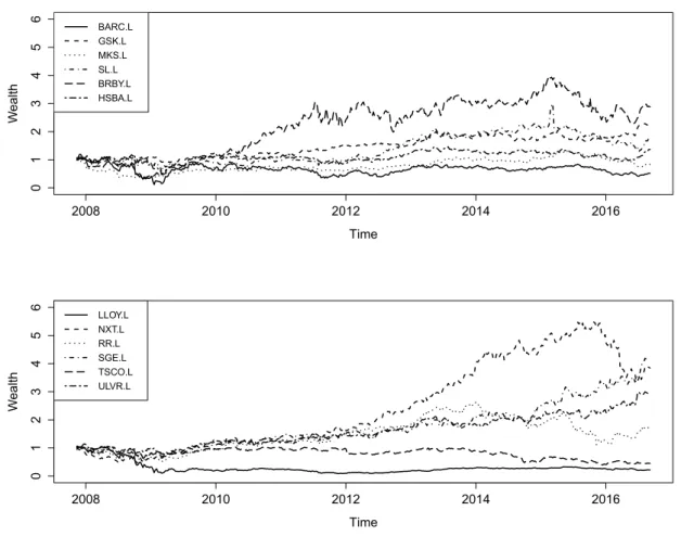
In this section, we discuss the procedure of a typical Bayesian portfolio selection. On the basis of her forecast of future stock returns, she optimally allocates the

Based on the normality assumption and on ¯ r and S as plug-in estimates, the distri-.. This will cause large short positions in the constructed portfolio. In the following, we