Testing Homogeneity of Time-Continuous Rating Transitions

Testing Homogeneity of Time-Continuous Rating Transitions

Rafael Weißbach*

, Patrick Tschiersch**, and Claudia Lawrenz**

*Institute of Business and Social Statistics, University of Dortmund, Dortmund, Germany

**Credit Risk Management, WestLB AG, Düsseldorf, Germany

August 23, 2005

Abstract

Banks could achieve substantial improvements of their portfolio credit risk assessment by estimating rating transition matrices within a time-continuous Markov model, thereby using continuous-time rating transitions provided by internal rating systems instead of discrete-time rating information.

A non-parametric test for the hypothesis of time-homogeneity is developed. The alterna- tive hypothesis is multiple structural change of transition intensities, i.e. time-varying transition probabilities. The partial-likelihood ratio for the multivariate counting process of rating transitions is shown to be asymptotically χ

-distributed. A Monte Carlo simu- lation finds both size and power to be adequate for our example. We analyze transitions in credit-ratings in a rating system with 8 rating states and 2743 transitions for 3699 obligors observed over seven years. The test rejects the homogeneity hypothesis at all conventional levels of significance.

†address for correspondence: Institute of Business and Social Statistics, University of Dortmund, 44221 Dortmund, Germany

email: Rafael.Weissbach@uni-dortmund.de, Phone: +49 231 755 5419, Fax: +49 231 755 5284.

JEL subject classifications. C51, G11, G18, G33.

Keywords: Portfolio credit risk, Rating transitions, Markov model, time-homogeneity, partial likelihood

1. Introduction

Among banks the interest in the estimation of rating transition matrices is rising. Sev- eral applications in risk management, like portfolio models for internal bank steering or pricing of credit risky financial products like CDS and CDOs need improvement. Addi- tionally, the Basel II accord (c.f. Basel Commitee on Banking Supervision(2004)) stimulates methodological advances in measuring credit risk. Planning to calculated regulatory capital with the internal ratings-based approach (IRB) within Basel II, banks have developed internal rating systems. By this means banks are provided with continu- ous-time observations of rating transitions of their obligors leading to new facilities in analyzing rating transitions. This data allows for a more precise estimation of rating transition matrices than discrete-time rating migration information published by external rating agencies like Standard & Poor’s.

For the estimation of transition matrices in discrete time the common ‘cohort method’ is used. It can be argued that transition probability estimates are only non-zero when direct rating transitions within the interesting time period have been observed. Defaults in the top ratings are likely to be considered impossible even though there clearly exists a risk of defaulting, at least through a series of successive downgrades. Transition probabili- ties are underestimated. These drawbacks become obsolete within continuous-time modelling.

Whereas Lando/Skødberg (2002) reject even the Markovian property for rating transi- tions, an additional assumption for the Markov model is critical - in both, discrete and continuous modelling -, time-homogeneity, leading to time-independent transition prob- abilities. Being exposed to two obligors over one year is the same as exposure in one of them over two years. The assumption not only has implications for the forecast of the default, and the consequent price of debt but also for the estimation of the actuarial probability using historical data. Assuming time-homogeneity in the continuous model implies that the intensity for changing the rating class does stay the same over time. In a time-homogeneous Markov model estimating transition matrices reduces to the estima- tion of the generator. Due to the reduced parameter space much more efficient estimates are accomplished compared to the more complex inhomogeneous model.

We address the two related topics: (i) Selecting the right Markov model for rating tran- sitions. (ii) Choosing between two estimation procedures. Therefore, we develop a par- tial-likelihood ratio test for the hypothesis of the homogeneity against the alternative of structural changes.

Having a notion of time one needs an origin. Time since issuance of the debt is a natural

choice for rating transitions, used e.g. by Calem/LaCour (2004) to assess portfolio credit

risk. Any (other) influence of the transition probabilities by covariates - like business

cycle, industry or domicile of the obligor (see e.g. Nickel et al. (2000), Lando/Skødberg (2002)) - is ruled out, in order to not assume a specific regression model. Access to an internal rating system with 8 rating states was granted by WestLB. This data covers the rating histories of 3699 obligors over seven years. The 2743 observed rating transitions lead to a clear rejection of the homogeneity. We compare the estimation of transition matrices for the homogeneous, i.e. reduced model and the full model and find substan- tial differences.

The paper is structured as follows: Section 2 reviews the Markov model and estimation techniques needed in the following. In Section 3 the test for homogeneity is constructed and asymptotic distribution is proven. Section 5 assesses the statistical properties of the homogeneity-test by simulation. In Section 6 real rating migrations are carefully ana- lyzed using the derived results. Section 7 concludes the paper.

2. Model

We model rating transitions of obligors as time-continuous Markov Processes, denoted by X : X , t = {

∈ T } and defined on a probability space ( , , P) Ω F and adapted to the fil- ration IF : = ( F

, t ∈ T ) . X

gives us the rating of the obligor at time t ∈ T = [0,T] ⊂

after the issuance of the credit. The possible rating states constitute the state space K = {1,..., k} where state 1 represents the highest rating and state k bankruptcy. A Markov process is determined by its transition matrix

(

)

P(s, t) : p (s, t) =

∈ , s, t ∈ T , s t ≤ , (1) where the transition probabilities p (s, t) P(X

=

= j| X

= h) h, j K ∀ ∈ give the prob- ability for a transition from rating h to j within the time period s till t. A time- homogeneous Markov processes additionally satisfies

P t s t P u s u

E (h(X ) | X ) E (h(X ) | X ) s, t, u

=

∀ ∈ T , where h : K → is an arbitrary func- tion. The corresponding transition probabilities only depend on the lag ψ = − t s . A quite useful property is stated by the Chapman-Kolmogorov-equation

P(s + t) = P(s)P(t) = P(t)P(s) ∀ ∈ s, t T . (2) Thus, if you know the one year transition matrix P(1) you will be able to calculate P(2), P(3) etc. simply by successive multiplication of P(1).

The link between time-homogeneous transition matrices P( ), ψ ψ ∈ T and the infini- tesimal generator is derived by transition intensities defined, in general, by

hj hj

hj 0

p (t, t ) p (t, t)

q (t) : lim , t ;h, j K

ψ→ +

+ ψ −

= ∈ ∈

ψ T , (3)

allowing for time-dependence, whereas, for the time-homogeneous case, the transition intensities become constant in time, i.e. q (t) q

≡

∈

t ∀ ∈ T ;h, j K ∈ , and are col- lected in the infinitesimal generator Q : q = ( )

∈

.

Now, the transition matrices can be expressed as a function of Q,

n

n 0

P( ) exp( Q) : ( Q)

n!

∞

=

ψ = ψ = ψ ∀ψ ∈T .

Thus, every transition matrix P( ψ ) can be estimated by the estimation of Q. Albert (1962) derives

n hj

hj T

0 h

N (T)

ˆq ,h j

Y (s)ds

•

•

= ≠ (4)

as maximum-likelihood estimator for the time-invariant transition intensities q ,h j

≠ if

0

Y (s)ds 0

> and sets ˆq : 0

= , otherwise.

It is common practice to assume that an obligor, once defaulted, cannot recover his business activity. Thus, default k is modelled as an absorbing state where

t s

P(X = k | X = k) 1 s, t = ∀ ∈ T , s t ≤ . This implies q

= ∀ ∈ 0 j K .

The relationship between intensities and transition matrices can be generalized to the inhomogeneous Markov process. P(s,t) may be expressed in terms of the cumulative transition intensities

0

A (t) : = q (s)ds h, j K : j h ∈ ≠ ,

j h

A (t) : A (t)

≠

= − by

( )

i i 1 i 0,....,n

k max |t t | 0 i k i i 1

(s,t]

P(s, t) (I dA) : lim I A(t ) A(t )

= −

− → −

= π + = ∏ + − ^{, (5)}

where s t = ≤ ≤ ≤ ≤ =

t

t

... t

t is a partition of the finite time interval [s,t] and π

denotes the so-called product integral (see Andersen et al.(1993), p.93).

Now we consider modelling rating transition histories X

,…,X

of a portfolio of i = 1,…, n obligors, where the lengths of the individual histories potentially differ. A suffi- cient statistics is the vector of original ratings X (0),...,X (0) and the multivariate

counting process N = ( N ( ), h j

⋅ ≠ ), where its components

( )

n n

hj hji i i

i 1 i 1

N (t) :

N (t) : #{s [0, t]: X (s ) h, X (s) j} , t , h j

= =

= = ∈ − = = ∈ T ≠ (6)

count the number of transitions from rating h to j until time t in the whole portfolio and

N (t)

for obligor i, respectively. For large portfolios this is a clear reduction regarding

the number of random processes.

The individual counting processes N (t)

are related to the corresponding cumulative transition intensities for transitions from rating h to j via their compensators Λ

(t) ,

t

hji

(t)

Y (s)dA (s)

Λ = , where Y (t) : I

=

(see Andersen et al.(1993), p.93).

Throughout the paper, we will assume absolutely continuous transition intensities q (t) 0 t

> ∀ ∈ T, j h ≠ , h ≠ k, implying a permanent risk of migrating from rating h to j.

This yields a multiplicative intensity process of N (t)

: λ

(t) q (t)Y (t) =

. For the portfolio based multivariate counting processes one gets the intensity process

hj

(t) q (t)Y (t)

λ = , where

i 1

Y (t) :

Y (t) n

=

= ≤ gives the number of obligors in rating h just before time t.

An estimator for the time-depending transition matrices P(s,t) can be constructed via equation (5) by just estimating the cumulative transition intensities A (t), j h

≠ . This is done by the Nelson-Aalen-estimator (see Nelson (1969))

h

t {Y (s) 0}

hj hj

0 h

ˆA (t): I dN (s), j h Y (s)

• >

•

•

= ≠ ,

j h

ˆ ˆ

A (t) A (t)

≠

= − (7) which Johansen (1978) proves to be the nonparametric maximum likelihood estimator for the cumulative transition intensities A (t), j h

≠ . This results in the non-parametric maximum likelihood estimator for P(s,t), the Aalen-Johansen estimator,

( )

i i 1 i 0,....,n

k max |t t | 0 k i i 1

u (s,t]

ˆ

ˆ ˆ

ˆP(s,t) (I dA(u)) lim I A(t ) A(t )

= −

− → −

=

π + = ∏ + − ^{, (8)}

where s t = ≤ ≤ ≤ ≤ =

t

t

... t

t denotes a partition of [s,t] (see Aalen/Johansen(1978), p.143). Expression (8) reduces to the discrete product

(

)

m

ˆ ˆ

ˆP(s,t) = ∏ I + µ − µ − A( ) A( ) ^{, where µ ∈}

T denotes the random time for the m- th of any rating transitions observed in the portfolio the rating state. The structure of the k x k-dimensional matrices A( ) A( ˆ µ − µ −

ˆ

) is described in detail by Lando/Skødberg (2002) (see p. 430-431).

3. Testing for Homogeneity

Our goal is to check if rating transition histories may be adequately modelled by a ho- mogeneous Markov model and transition probabilities, thus, exhibit time-invariant be- haviour. As shown in chapter 2, this is equivalent to constant transition intensities yield- ing a sparse parametrization of the Markov model by its generator. Therefore, the null hypothesis of time-homogeneity can be stated in terms of

hj hj hj

: h,j K: c ∀ ∈ ∃ ∈

: q (t) c t [0,T] = ∀ ∈

H

. (9)

We are interested in the alternative that transition probabilities are time-dependent which can be approximated by structural breaks of the transition intensities, i.e.

i 1 i 1 2

b b

hj i 1 hji [t ,t ) 1 2 hji hji

: h,j K: q (t) ∃ ∈ =

q I

(t) : i ,i ∃ = 1,..., b : q ≠ q

H

(10)

where 0 t = ≤ ≤ ≤ =

t

... t

T is a partition of T consisting of b intervals. The follow- ing test is based on likelihood theory and mimics already known homogeneity-tests in a discrete modelling framework (see Anderson/Goodman (1957), Kiefer/Larson (2004)).

First of all, following Andersen et al.(1993, p.296), we have to derive the partial- likelihood for n independent observations X

,…, X

of a time-continuous Markov process under the assumption of absolutely continuous transition intensities. Let the transition data for the portfolio be given by an observation of the multivariate counting process N with components defined in (6). Again, equation (5) allows to parametrize the model of a general Markov Process either by the transition matrices P(s,t) in (1) or the cumulative transition intensities A (t)

in the preceding section.

Given F

and a transition, the increments ( dN (t), j h

≠

) of N with fixed h at time

t are multinomially distributed with parameters ( Y (t),dA (t), j h

≠

) and independent over h = 1,..., k. Thereby the likelihood gets

( )

hj h h

hj hh

hj hj

dN (t) Y (t) dN (t)

h hj hh

h K j h q (t)dt q (t)dt

t [0,T]

L A (t) | N (t), j h;h,j K;t [0,T]

Y (t)dA (t) 1 d A (t)

• ••

•

−

∈ ≠

∈

≠ ∈ ∈

= π ∏ ∏ + ⁽¹¹⁾

where

j 1 i 1 j h

N (t) :

N (t)

= =

≠

= . To ensure the likelihood is valued greater than zero, even when Y (t) 0

= meaning that no obligor is left in a rating state h , we define 0 : 1

= . The test statistic of the likelihood ratio test for the preceding test problem is

(

)

: 2ln(LR) 2 ln L ln L

Φ = − = − − , (12)

and incorporates the likelihood ratio,

( )

( )

0 hj

hji

H hj hj

q , j h 0

1 hj hj

q ,i 0,...,b 1;j h

sup L q | N (t), j h;h,j K;t [0,T]

LR : L

L sup L A (t) | N (t), j h;h,j K;t [0,T]

≠ •

= − ≠ •

≠ ∈ ∈

= =

≠ ∈ ∈ ^{, (13)}

which compares the maximized likelihood under the null of time homogeneity versus

the likelihood when maximizing under the alternative of structural breaks of q (t)

.

Using standard theorems of likelihood testing, as layed out in Serfling (1980), for in-

stance, Φ is, under the null, asymptotically χ

-distributed with d = D

– D

degrees of

freedom where D

and D

are the dimensions of the parameter space under the null and the alternative, respectively. Modelling an absorbing default state the degrees of free- dom are d (b 1) (k 1) = − ⋅ −

.

The actual value of the likelihood ratio LR in (13) can be calculated by inserting in the likelihood in (11) the ML-estimators for the transition intensities q (t)

under the null and the alternative, if they exist. Assuming time homogeneity, the ML-estimator for the constant transition intensities is ˆq in (4) (see last section) and thus determines L

. With respect to the fact that transition intensities q (t)

=

q I

(t), h j ≠ are par- tially constant under the alternative we could also apply this estimator to derive the ML- estimator for q (t) . Therefore, we only have to find ML-estimators for the b parameters

q ,i ,..., b

= of the step functions q (t) . This could be accomplished by confining the

considered time interval, where rating transitions are observed, from [0,T] to the i-th time interval [t

, t )

of the partition of [0,T]. Thereby, the ML-estimator of

q ,i ,..., b

= is given by

i

i i 1

i 1

hj i hj i 1 t

nhji t t h

t h

N (t ) N (t )

ˆq , for Y (t)dt 0

Y (t)dt

−

• • − −

− − •

− •

− − −

= >

It could be regarded as the ML-estimator ˆq for a time homogeneous Markov process

on this restricted time interval, and thus only takes into account rating transitions that occur within [t

, t )

.

Finally, we want to point out that the likelihood ratio LR in (13) could be computed efficiently by using the ‘Poisson likelihood’,

(

) (

)

j h

t [0,T] h K j h 0

L A (t) | N (t)

Y (t)dA (t)

exp Y (t)dA (t)

≠

∈ ∈ ≠

≈ ∏ ∏∏ − ^,

as an approximation for the likelihood in (11), as suggested by Andersen et al.(1993), p.

297. Therefore, LR in (13) could be approximately calculated by

hj

i 1 i

dN (t) b n

hj i 1 t [t ,t ] h K j h nhji

LR ˆq : LR

ˆq

•

= ∈ − ∈ ≠

≈ ∏ ∏ ∏∏ = ⁽¹⁴⁾ where no product integral has to be calculated. LR is well defined, because the estimate

n

ˆq is only zero when no transition from rating h to j occurs within

[t

, t )

. Then there is clearly no jump in the counting process N

yielding dN (t) 0 t [t , t )

= ∀ ∈

, so that the inner factor becomes ( )

( ) ( )

( )

hj

hj

dN (t) 0

n n

hj hj

dN (t) 0

nhji

ˆ ˆ

q q 1

1 1 ˆq 0

•

•

= = = for t [t , t ) ∈

.

By restricting the class of alternatives to structural breaks in transition intensities the power of the test for homogeneity has been increased. We are able to get better feeling of this special term structure which captures a lot of other possible functional forms, even then when only a few rating transitions are observed, as is usual in practice.

Whereas, testing against a broad class of inhomogeneous models as alternative would require a considerable large amount of observed rating transitions.

4. Some Monte Carlo Simulations

As the test for homogeneity of time-continuous rating transitions presented in chapter 4 is an asymptotical test we carry out a Monte Carlo simulation to assess its finite sample properties. Therefore, we determine the probabilities for the type I and type II errors for the test based on the test statistic Φ defined in (12). To reduce complexity we simulate from a time-homogeneous Markov model on a binary state space K = {0, 1} where 0

denotes any non default-rating and 1 denotes bankruptcy, thus only accounting for de- faults of obligors. When modelling an absorbing default state q (t) 0 t [0,T]

= ∀ ∈ holds and the default model is parametrized by only one transition intensity, q (t) . The

null of time homogeneity becomes H

: q (t) c

= ∈

t [0,T] ∀ ∈ . Here, it should be tested against the specific alternative that q (t) exhibits a structural break at T/2, for-

mally

0

1 01 0 1

1 0

c ,0 t T

: q (t) 2 ,c ,c

c c , T t T 2

+

≤ <

= ∈

≠ ≤ ≤

H .

We use the following technique to simulate a portfolio of n obligors whose transition histories are assumed to be generated by the same Markov process X on the state space K with given transition intensities

q (t) . It is sufficient to know the default times

i

[0,T]

τ ∈ of each obligor i = 1,…, n, because that is the point in time when X

jumps to one before it was constantly zero. We have to simulate a sample τ = τ ( ,..., )

τ

of de- fault times with the distribution function

(

)

F(t) 1 exp = − − q (s)ds , t ∈

. (15)

To analyze the actual size of the homogeneity test based on Φ we simulate

n

= 20,000 such samples τ of default times under the null of homogeneous rating

transition histories corresponding to a one year probability of default PD

= F(1) of 1

percent – or c = -ln(0.99) –, i.e. a mediocre rating class of ‘BB’ in the Standard &

Poor’s system.

The power of the LR-test is studied by simulating n

= 20.000 such samples τ under the special alternative where the transition intensity is given by

01 [0,T / 2) [T / 2,1]

q (t) = − ln(0.99)I (t) 2ln(0.99)I − (t) , the intensity doubles half way.

Table 1 shows the actual size under the null and the power under the alternative, respec- tively for different sample sizes n. In each iteration step of the simulation the homoge- neity test on significance level α = 0.05 is carried out by calculating the LR test statistic

Φ approximately using LR in (14).

Sample size n Size

Power 30 0.00560 0.01705 300 0.08865 0.20375 3,000 0.05265 0.89505 30,000 0.05025 1.00000

Table 1: Simulation of actual size α

and power β of approximate likelihood ratio test for the null of constant hazard rate versus structural break at T/2 (n

= 20,000 simulation runs, significance level α = 0.05)

The approximate LR test based on Φ = − : 2ln(LR) shows, to some extent, an anticon- servative behaviour because of the values of the size which are slightly higher than the significance level 0.05. This means that the LR-tests tends to reject the null of time- homogeneity a bit too often. But when the sample size n → ∞ , α * seems to converge to α , as the difference between α

and α gets negligibly small. Moreover, the test seems to be consistent against the tested alternative because apparently the power in- creases when the sample size n gets larger. Already in the case of n = 3000 obligors the null of time homogeneity is rejected correctly in nearly 90 percent of all cases, even though the true hazard rate has only one structural break and thus only shows somewhat moderate deviations from the null. Bearing also in mind that a one-year PD of 1 per-

cent and a two-year PD

= − 1 exp( 0.03) 0.0297 − = is definitely not unrealistic, but is a valid value for ratings ranging from mediocre to poor.

Summing up, this simulation study clearly provides no evidence that undermines the

appropriateness of the approximate LR-test on time-homogeneity of time-continuous

rating transition histories. These results can be transferred to a general model for rating

transitions with more than one parameter under test when there are enough transition

intensities which are not constant, what is a likely scenario.

5. Empirical Results

We now show how to analyze time-continuous rating transitions as observed by banks within their internal rating systems using the methodological results derived in chapter 2 till 4. Our main objective is to accurately estimate rating transition matrices. Therefore, we answer the question whether rating transitions could be modelled by a time- homogeneous Markov model or dependence on the time since issuance of a credit has to be taken into account by applying the approximate LR-test for homogeneity presented in chapter 4. After selecting the ‘right’ model we present the results of the subsequent estimation procedure described in chapter 3, either estimating the generator Q which parametrizes the less complex homogeneous model or estimating the time-dependent transition matrices P(s,t) of the general inhomogeneous model directly by the Aalen- Johansen-estimator. Then we compare it with the other estimation procedure, poten- tially in question when not testing beforehand.

The data

WestLB AG granted access to an internal rating system with 8 rating states where 1 denotes the internal top rating and 8 the poorest rating of an obligor, and a default state 9. Rating histories were observed over seven years from 1.1.1997 until 31.12.2003. To use the time since issuance we restricted our analysis to a portfolio comprising 3699 global obligors of WestLB that entered the portfolio after the start date of the observa- tion. In this portfolio 2743 rating transitions, including transitions to default, occurred within that period. When a rating change took place exact dates were recorded. Figure 1 gives insight to what extent obligors tend to change their ratings.

Figure 1: Empirical distribution of the number of rating transitions per obligor during the indi-

vidual rating history over maximal seven years

This simple statistic underpins that rating transitions are quite rare credit events. The creditworthiness of even a half of the analyzed counterparties does not change anyway.

Per year an obligor changes his rating on the average only 2743/10641.6 = 0.26 times.

Results of test for homogeneity

Now we focus on the question whether a time-homogeneous Markov model is suitable for the rating transitions histories of the 3699 obligors in the analyzed portfolio. The actual test statistic Φ is approximated by Φ = − : 2ln(LR) as done before in the simula- tion in chapter 5. We are interested in testing the null of time-homogeneity set out in (9) at the significance level 0.05 against the alternative of transition intensities with struc- tural breaks, given in (10). We consider different equidistant partitions

0 1 2 b

0 t = ≤ ≤ ≤ ≤ = t t ... t 7 of the time interval [0,7] containing all times since issuance when ratings of any obligor in the portfolio changed. The maximal number b of breaks is set to seven yielding seven one-year intervals where transition intensities could vary.

The test results in this setting are given below in Table 2.

Number b of structural

breaks 2 3 4 5 6 7

Test statistic 93.8513 125.9231 289.2518 345.8185 447.2865 626.1497 p-Value 0.0089 0.5354 < 0.0001 0.0002 < 0.0001 < 0.0001 Table 2: Results of approximate LR-test for homogeneity using Φ = − : 2ln(LR) as test statistic

analyzing a WestLB-portfolio of 3699 obligors with rating histories observed within maximal seven years since issuance of credit

These strikingly small p-values show that the time since issuance does influence rating transition probabilities significantly. More granular partitions do not necessarily give smaller p-values, as the number of parameters to be estimated increases but the gain of precision in the approximation of continuous transition intensities declines.

Additionally, we could also reveal time-varying transition probabilities by analyzing the term structure of the Nelson-Aalen-estimator ˆA (t),h j

≠ in (7) for the cumulative tran- sition intensities A (t)

. If rating transition histories of the WestLB-portfolio really are homogeneous A (t)

would show a linear relationship with the time since issuance.

Thereby, in figure 2 we graphically check for deviations of ˆA (t),h j

≠ from a charac-

teristic linear curve.

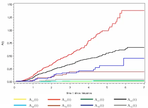
Figure 2: Nelson-Aalen-estimator ˆA (t),h j

≠ for cumulative transition intensities for various rating combinations plotted against time t since issuance of credit

It is evident that patterns of cumulative transition intensities differ substantially when analyzing transitions out of ratings with different quality, here ratings 2, 4, and 7. The more pronounced slope for transitions in neighbouring ratings, e.g. for transitions from rating 2 to 3, means that the risk of migrating instantly to a rating nearby is all the time much higher than migrating to distant ratings. With 2090 transitions, indeed the vast majority of a total 2743 transitions are targeted to a direct neighbour rating.

There seems to be no global trend in the transition intensities since the ˆA (t),h j

≠ have no gradient which increases over the whole period [0,7]. Rather, there are local different slopes for all analyzed cumulative rating transition intensities. Especially the flat curve at the beginning points to a reduced risk of migrating since only a few transi- tions occur up to one year after the issuance, even though the number of obligors in the starting phase is higher than in other periods. Thus, the rejection of homogeneous transi- tions as a result of the LR-test is confirmed by the non-linear term structure of the esti- mated cumulative transition intensities.

This term-structure gives an explanation for the p-value of 0.0089 when b = 2 which is somewhat greater than for b 4 ≥ and that the test for b = 3 even fails to reject the null (p-value = 0.5354). These partitions are too rough to detect these deviations from the null of homogeneity, because the average of transition intensities over longer periods smoothes the different levels.

These findings point out the main drawback of the LR-Test to detect structural breaks:

The test results depend on the choice of the number b of structural breaks. Since the

A (t)21

number of parameters q ,i 1,..., b

= under the alternative increases by k(k 1) (k 1) (k 1) − − − = −

, here by 64, each time when dividing [0,T] by one more in- terval we recommend to choose b with respect to the size of the portfolio and the length of the partition intervals. Because the number of transitions could fall below the number of parameters to estimate under the alternative very fast, resulting in highly inefficient estimators ˆq

for the parameters of the transition intensities

i i 1

b b

hj i 1 hji [t ,t )

q (t) =

q I

(t), h j ≠ .

In our example we find it doubtable to estimate more than 588 parameters with 2743 observed rating transitions, since transitions into ratings far away from the current rat- ing, say from rating 1 to default, are expected to be fairly unlikely. Moreover, dividing the observation horizon [0,T] into seven one-year intervals seems to be appropriate as we intend to analyze long-term changes in the transition probabilities instead of short- term variations, i.e. how much changes the one-year probability for a transition from rating h to j if an obligor is already three years in our portfolio in contrast to the period immediately after issuance.

Surely one can argue that the influence of the time since issuance of a credit stated here is in fact induced by other covariables like domicile or industry of the obligor as figured out in other empirical studies like Nickell et al. (2000). Indeed, a bias could appear if the structure of the portfolio concerning these variables changes over time. For instance, the proportion of obligors in a certain rating that are in the telecommunications industry is in the period up to one year after issuance small and then rises, because the deals of the bank with these obligors last longer than in other industries. If there really is an in- dustry effect which causes different migration risks over the same time horizon in dif- ferent industries this could induce time-varying transition intensities.

To preclude this undesirable effect we checked the structure of the portfolio in different time periods for the covariables domicile and industry and found no such striking im- balance which undermines this analysis and its results. Since we only observed transi- tions over a time period of seven years rating changes for obligors that are already longer in the portfolio, necessarily, all took place in a recessive phase of the business cycle, whereas ratings for obligors, that have been only for a short time in the portfolio of WestLB, are also observed in other business environments before the millennium.

Analyzing rating transition probabilities

The clear rejection of the null of homogeneous rating transitions points to estimate tran-

sition matrices by the Aalen-Johansen-estimator to account for the term structure of

transition probabilities. This shows up when analyzing transition probabilities for a

fixed period, say one year, graphically in figure 3.

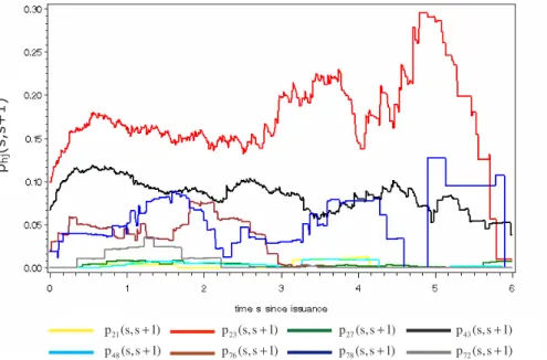
Figure 3: One-year transition probabilities p (s,s 1), h, j K

+ ∈ for various rating combinations h,j plotted against time s since issuance of credit

Probabilities P(s,s 1) + for transitions within one year vary more or less pronounced when time s since issuance evolves. All analyzed transitions have in common that prob- abilities rise sharply during the first year. For instance, probabilities for transitions from rating 2 to 3 double from 10 to 18 percent. But their levels depend heavily on the qual- ity of the rating and the distance between start- and end-rating, because transitions into the direct neighbour rating are much likelier than those into distant ratings.

Furthermore, there are only local and no global trends which is in line with the term structure of the cumulative transition intensities in figure 2. Nevertheless, the transition probability p (s,s 1)

+ from rating 2 to 3 tends to increase up to s = 5 years and then immediately drops from a high level of 30 percent. The high jumps in the probabilities for transitions out of rating 7 came from the fact that there are less obligors in this rat- ing. Similar results could be found for transition probabilities for other rating combina- tions and other time-horizons.

Tables 3 and 4 present the estimation results for the one-year transition matrices P(0,1) and P(1,2) using the Aalen-Johansen-estimator ˆP(0,1) and ˆP(1,2) , respectively, given in (8). Due to the security policy of WestLB we have to omit the PD-column and the diagonal-elements of the transition matrices. But the results of the analysis also apply to the PDs.

p (s,s 1)21 + p (s,s 1)23 + p (s,s 1)27 + p (s,s 1)43 + p (s,s 1)48 + p (s,s 1)76 + p (s,s 1)78 + p (s,s 1)72 +

Rating 1 2 3 4 5 6 7 8

1 0.00 0.00 0.01 3.20 0.00 0.01 0.00

2 0.00 9.90 2.59 0.11 0.01 0.01 0.00

3 0.00 1.88 7.58 0.65 0.15 0.08 0.01

4 0.00 0.60 6.68 5.67 0.41 0.13 0.03

5 0.18 0.05 2.76 11.42 2.97 1.20 0.68

6 0.00 0.03 0.36 4.83 6.06 2.65 0.80

7 0.00 0.01 0.16 3.23 3.98 2.00 1.86

8 0.00 0.00 0.01 0.20 3.03 1.50 3.89

Table 3: Aalen-Johansen-estimator ˆP(0,1) for one-year rating transition matrix P(0,1) at time of issuance of credit (in percent)

Most of the estimated probabilities for transitions within one year after time of issuance in table 3 are positive, even though neither every rating transition was observed directly nor indirect rating changes by the same obligor necessarily took place. The Aalen- Johansen-estimator P(s,t) captures migration risk for transitions from r to

r , as long as

there exists a sequence of ratings r ,r ,...,r , r

where at least one of the n obligors migrates from the preceding to the subsequent rating within the regarded time period [s,t], i.e. N

(t) N −

(s) 1 i 1,..., m 1 ≥ ∀ = − . The concentration of zero-estimates for transitions into and out of rating 1 stem from the fact that there were no such transitions in the portfolio up to one year, i.e. N

(1) = 0 and N

(1) = 0 for h, j = 2, 3, 6, 7, 8.

Since the transition probabilities almost never exceed 10 percent and the PDs, in most ratings, could be expected to be quite smaller there is a chance of about 80 percent to stay in the same rating for one year after the issuance. If albeit a rating change occurs it is very unlikely to migrate in a distant rating since the transition probability for migrat- ing in a neighbour rating is the highest one, except for ratings 1 and 7. As the distance between current and target rating increases the transition probabilities decreases very fast. For instance, obligors in rating 5 have a chance of 11.4 percent to be upgraded by one rating category, but only a chance of 2.8 percent for an upgrade to rating 3. This structure of the one-year transition matrix reflects the rating policy of banks that adapt ratings rather in small steps within short time periods than with one rating change of more categories after some time.

Moreover, the quality of the current rating influences the direction of the migration. We have to distinguish between a pronounced downgrade risk in the ratings 1, 2, 3 with high quality and an upgrade tendency in the ratings 4, 5, and 6. In these ratings always transitions into the next rating in the direction, pointed out before, are most likely.

WestLB’s rating system is calibrated in such way that in the poor ratings 7 and 8 default risk is predominant.

Comparing the estimated one-year transition matrices P(0,1) at time of issuance in table

3 and P(1,2) after one year in the portfolio in table 4, it could be stated that the transi-

tion probabilities for changing the rating within one year differ considerably when an obligor was already one year in the portfolio.

Rating 1 2 3 4 5 6 7 8

1 0.15 3.81 4.69 2.71 0.13 0.18 0.05

2 0.33 15.93 5.56 2.93 0.75 0.81 0.06

3 0.21 3.04 14.23 3.30 0.49 0.52 0.09

4 0.32 0.82 11.12 8.83 1.18 1.30 0.45

5 0.42 0.54 2.72 14.97 3.16 4.39 0.73

6 0.06 0.20 0.52 6.67 13.05 11.13 1.28

7 0.05 2.26 1.91 6.37 4.98 4.55 5.07

8 0.01 0.04 0.04 0.24 2.18 2.17 2.33

Table 4: Aalen-Johansen-estimator ˆP(1,2) for one-year rating transition matrix P(1,2) at one year since issuance of credit (in percent)

Foremost, the difference arises because nearly all transition probabilities p (1, 2), h j

≠ are remarkably higher than the counterparts p (0,1)

at time of issuance where the maximum difference of 0.084 is observed for a downgrade from rating 6 to 7. This means that in general there is a higher migration activity in the second year after enter- ing the portfolio. This leads to even higher downgrade risks in the high ratings 1, 2, and 3 and likewise to more pronounced upgrade chances in the ratings 4,5, and 6, as transi- tions to more distant ratings become more likely after obligors have spent one year in the portfolio. But downgrade risk in rating 7 is not any longer predominant. Moreover, no transition probability is estimated with zero.

We emphasize that it makes a difference still presuming time-homogeneity erroneously since estimation results of homogeneous matrices via the generator differ substantially.

The estimation Q : q ˆ = ( ) ˆ

of the generator Q is given below in Table 5, where its components are estimated by (4).

Rating 1 2 3 4 5 6 7 8

1 0.00 2.12 1.06 5.30 0.00 0.00 0.00

2 0.19 18.83 4.29 1.21 0.47 0.28 0.00

3 0.11 3.18 15.37 2.40 0.62 0.43 0.05

4 0.09 0.62 11.11 9.75 1.51 0.77 0.33

5 0.19 0.25 3.11 16.50 5.08 3.24 0.70

6 0.00 0.31 0.31 5.29 13.39 12.45 0.93

7 0.00 0.98 0.33 3.60 5.90 4.26 5.90

8 0.00 0.58 0.00 0.00 1.74 2.31 4.63

Table 5: Maximum-likelihood-estimation ˆQ for the infinitesimal generator Q (in percent)

The resulting estimation ˆP(1) of the homogeneous transition matrix P(1), presented in

table 6, for ratings within one year at any time after the issuance are calculated via the

Taylor-type expansion mentioned in section 2. All entries q , h, j K

∈ of ˆQ , estimated with zero, are caused by the fact that no obligor migrated from rating h to j over the whole observation period, i.e. N

(T) = 0. Even though, all transition probabilities in

ˆP(1) are positive.

Rating 1 2 3 4 5 6 7 8

1 0.04 1.95 1.40 4.45 0.12 0.08 0.02

2 0.17 15.06 4.58 1.33 0.45 0.31 0.03

3 0.10 2.55 12.35 2.49 0.62 0.46 0.09

4 0.09 0.64 8.93 7.61 1.34 0.82 0.31

5 0.17 0.30 3.14 12.86 3.81 2.73 0.65

6 0.01 0.31 0.70 4.95 10.12 9.27 1.01

7 0.01 0.80 0.58 3.30 4.82 3.29 4.55

8 0.00 0.47 0.09 0.25 1.54 1.81 3.67

Table 6: Estimated homogeneous one-year transition matrix ˆP(1) derived by estimated generator ˆQ (in percent)

The homogeneous one-year transition matrix shows differences to both inhomogeneous matrices P(0,1) and P(1,2), analyzed before. It is not surprising that the homogeneous transition probabilities p (1), h, j K

∈ are higher than the probabilities p (0,1)

for the same transitions at issuance and also lower than the one-year probabilities p (1, 2)

at one year. Since P(1) is based on the generator all migration information is incorporated in the estimation. As pointed out before, the generator averages the time-varying transi- tion intensities therefore generating a transition matrix which also neglects the discrep- ancies in time-depending transition matrices for the same time-horizon ψ . Although the level of transition probabilities is different, the structure of the matrix ˆP(1) , concerning the predominant up- and downgrade tendencies in ratings 4, 5, 6 and ratings 1, 2, 3 re- spectively, remains stable.

Finally, we analyze graphically how rating transition probabilities change when looking at different time-horizons within which rating changes occur. Homogenous transition probabilities p ( ), h, j K

ψ ∈ , plotted in figure 4, increase as time-horizon ψ is ex- tended, at least up to a six-year horizon. This empirical result is theoretically backed by the Chapman-Kolmogorov-equation P(s + t) = P(s)P(t) = P(t)P(s) ∀ ∈ s, t T in (2).

Thereby, with rising time-horizon it gets more likely that obligors arrive at a certain

rating through a sequence of rating changes.

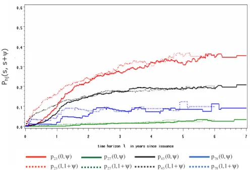
Figure 4: Homogeneous transition probabilities p ( ) h, j K

ψ ∈ for various rating combinations h,j plotted against time horizon ψ

Again, rating transition probabilities into direct neighbouring ratings, i.e. 2 to 3, 4 to 3, 7 to 8 and 7 to 6, excepting ratings from 2 to 1, clearly dominate probabilities for transi- tions in ratings far away like 4 to 8. Within that group transitions from 2 into 3 and 4 to 3 are much likely since the probabilities for periods of more than one year permanently exceed 10 percent and even rise up to 20 and 30 percent, respectively. Whereas, prob- abilities for transitions from 7 to 8 reach its maximum of only 8.5 percent for ψ = 4.9 years. Probabilities for transitions into distant ratings here never exceed the 2.6 percent.

The stylized, smooth evolution comes from the calculation via the generator Q. Here the grouping of the transition probabilities remains stable as the time-horizon increases.

Time-inhomogeneous transition probabilities p (s,s

+ ψ ) also increase with rising time-horizon ψ when starting date s is fixed as seen in figure 5. But there could be lo- cal downturns due to statistical variations in the estimations since every p (s,s

+ ψ ) are estimated separately for each point t s = + ψ in time using the rating transition which recently occurred.

The largest differences between transition probabilities at time s = 0 and s = 1 could be observed for short periods up to 1.5 years where for instance the probabilities for transi- tions from 2 to 3 at s = 1 year in the portfolio increase sharply and reaches the level of nearly 8 percent for time-horizons of ψ = 4 month, whereas the same probabilities at issuance are only that high for time horizons of one year. For larger time-horizons tran- sition probabilities at different points in time behave rather similar.

ψ

ψ

p ( )21ψ

Figure 5: Transition probabilities p (s,s

+ ψ ) h, j K ∈ for various rating combinations h,j and starting times s = 0, 1 after time of issuance plotted against time horizon ψ An interesting result is that the inhomogeneous transition probabilities approach the level of their homogeneous counterparts as the time-horizon increases. This is feasible since both estimation techniques use in the end completely the same migration data.

6. Conclusion

Homogeneity of rating transitions simplifies the application of transitions matrices to credit risk valuation. Moreover, estimating the parameters for the Markov model is effi- cient. Statistical inference allows to discriminate the homogeneity from the converse on basis of a representative historical sample. Our rating history rejects the homogeneity hypothesis in favour of level changes of the (constant) transition intensities at prede- fined breaking times. In the homogeneous model, observing the debt from the origin of time is not necessary. The deeper reason is the lack of memory of the exponential distri- bution, the univariate provenience of the homogeneous Markov process. Measuring time with respect to a calendar is possible. The inhomogeneous model calls for a differ- ent origin of time. We propose to measure time since issuance of the debt, e.g. the be- ginning of a loan contract in commercial lending and adopt hereby the view of a portfo- lio owner, a bank, forecasting its (portfolio) credit risk.

We find e.g. that transitions in the first year (of lending commitment) are less frequent than in the second, and that the one-year estimate based on homogeneity ranges in be- tween. As a consequence, forecasting portfolio credit risk with rating-transition prob- abilities for a one-year horizon with the homogeneity assumption overestimates the risk,

p (0, )23 ψ

ψ

ψ

e.g. the economic capital, for a portfolio of ``fresh’’ exposures and underestimates the risk if all exposure have been originated one year ago. The portfolio composition with respect to the age of debt needs to be taken into account, not only for the internal portfo- lio model but also for regulatory capital under Basel II. The study confirms a significant covariable for credit risk also found in discrete modelling by Calem/LaCour (2004).

However, the detection of the right model for rating transitions is beyond the scope of this study. Inhomogeneity is not sharp, modelling the transition mechanism in accor- dance with the historical evidence needs careful selection of transition-intensity models.

Our nonparametric estimate is only the least restrictive approach and does e.g. not fit the need for forecasts of transitions in the distant future.

Acknowledgement: We acknowledge the financial support of DFG, SFB 475 ``Reduc- tion of Complexity in Multivariate Structures", project B1. The views expressed here are those of the authors and do not necessarily reflect the opinion of WestLB AG.

References

AALEN, O.; JOHANSEN, S. (1978): An empirical transition matrix for nonhomogene- ous Markov chains based on censored observations, Scandinavian Journal of Statis- tics 5, 141-150.

ALBERT, A. (1962): Estimating the infinitesimal generator of a continuous time, finite state markov process, Annals of Mathematical Statistics 38,727–753.

ALTMAN, E.I.; KAO, D. (1992): Rating drift of high yield bonds, Journal of fixed in- come 2, 15-20.

ANDERSEN; P., BORGAN, Ø.; GILL, R.; KEIDING, N. (1993): Statistical Models Based on Counting Processes. Springer, New York.

ANDERSON, T.W.; GOODMAN, L.A. (1957): Statistical Inference about Markov Chains, Annals of Mathematical Statistics 28, 89-110.

CALEM, P.S.; LACOUR-LITTLE, M. (2004): Risk-based capital requirements for mortgage loans, Journal of Banking and Finance 28, 647-672.

JOHANSEN, S. (1978): The product limit estimator as maximum likelihood estimator, Scandinavian Journal of Statistics 5, 195-199.

LANDO, D.; SKØDBERG, T. (2002): Analyzing rating transitions and rating drift with continuous observations, Journal of Banking & Finance 26,423–444.

KIEFER, N.M.; LARSON, C.E. (2004): Testing Simple Markov Structures for Credit Rating Transitions, U.S. Treasury Office of the Comptroller of the Currency Eco- nomics Working Paper, No. 2004-3.

NELSON, W. (1969): Hazard plotting for incomplete failure data, J. Qual. Technol. 1, 27-52.

NICKELL, P.; PERRAUDIN, W.; VAROTTO, S. (2000): Stability of rating transitions, Journal of Banking & Finance 24, 203-227.

SERFLING, Robert J. (1980): Approximation theorems of mathematical statistics. J.

Wiley, New York.