Slow transport by continuous time quantum walks

Slow transport by continuous time quantum walks

Oliver Mülken*and Alexander Blumen^†

Theoretische Polymerphysik, Universität Freiburg, Hermann-Herder-Straße 3, D-79104 Freiburg i.Br., Germany (Received 9 August 2004; published 3 January 2005)

Continuous time quantum walks(CTQWs)do not necessarily perform better than their classical counter- parts, the continuous time random walks(CTRWs). For one special graph, where a recent analysis showed that in a particular direction of propagation the penetration of the graph is faster by CTQWs than by CTRWs, we demonstrate that in another direction of propagation the opposite is true. In this case a CTQW initially localized at one site displays a slow transport. We furthermore show that when the CTQW’s initial condition is a totally symmetric superposition of states of equivalent sites, the transport gets to be much more rapid.

DOI: 10.1103/PhysRevE.71.016101 PACS number(s): 05.60.Gg, 05.40.⫺a, 03.67.⫺a

The transfer of information over discrete structures (net- works)which are not necessarily regular lattices has become a topic of much interest in recent years. The problem is rel- evant to many distinct fields, such as polymer physics, solid state physics, biological physics and quantum computation (see Refs.[1–6]for reviews). In particular, quantum mechan- ics seems to allow a much faster transport than classically possible. Thus, recent studies of quantum walks on graphs show that these often outperform their classical counterparts, i.e., in terms of the penetrability of the graph (for an over- view see Ref.[4]and references therein). We recall that the extension of classical random walks to the quantum domain is not unique. There exist different variants of quantum walks, such as discrete[7]and continuous time[8]versions, which are not equivalent to each other. Here we focus on walks in continuous time.

Walks occur over graphs which are collections of con- nected nodes. To each graph corresponds a discrete Laplace operator (sometimes also called adjacency or connectivity matrix), A =共A_ij兲. Here the nondiagonal elements A_ij equal

−1 if nodes i and j are connected by a bond and 0 otherwise.

The diagonal elements A_ii equal the number of bonds which exit from node i, i.e., A_ii equals the functionality f_i of the node i.

Classically, assuming the transmission rates of all bonds to be equal, say ␥, the continuous-time random walk (CTRW)is governed by the master equation[6]

d

dtp_j共t兲=

兺

where p_j共t兲 is the probability to find at time t the walker at node j. T =共T_jk兲is the transfer matrix of the walk, which is related to the adjacency matrix by T = −␥A. Equation (1) is spatially discrete, but it also admits extensions to continuous spaces, e.g., leading to the disordered Lorentz gas model, which describes the dynamics of an electron through a dis- ordered substrate[9].

We stick with the spatially discrete situation and let now

the CTRW start from node k, i.e., we set p_k共0兲=␦jk. Denoting by p_jk共t兲the conditional probability of being at node j at time t when starting at node k at t = 0 leads to

d

dtp_jk共t兲=

兺

which is another way to write Eq.(1) [5,6]. Given the lin- earity of these equations, their solution involves a simple integration. For Eq.(2)we have formally

p_jk共t兲=具j兩e^Tt兩k典. 共3兲 We now turn to one quantum mechanical extension of the problem, the so-called continuous-time quantum walk (CTQW). CTQWs are obtained by assuming the Hamil- tonian of the system to be H = −T [8,10]. Then the basis vectors兩k典associated with the nodes k of the graph span the whole accessible Hilbert space. In this basis the Schrödinger equation reads

id

dt兩k典= H兩k典, 共4兲 where we set ប⬅1. The transition amplitude ␣jk共t兲 from state兩k典at time 0 to state兩j典at time t is then

␣jk共t兲=具j兩e^−iHt兩k典. 共5兲 According to Eq.(4)the ␣jk共t兲 obey

id

dt␣jk共t兲=

兺

The inherent difference between Eq.(3)and Eq.(5)is, apart for the imaginary unit, the fact that classically 兺jp_jk共t兲= 1, whereas quantum mechanically兺j兩␣jk共t兲兩²= 1 holds.

We turn now to the graph displayed in Fig. 1(a). The graph is obtained from two finite Cayley trees of generation G which have a common set of end nodes along the horizon- tal symmetry axis indicated in Fig. 1(a) [8,10]. For the nodes on the axis as well as for the top and bottom nodes the connectivity is f = 2, whereas for all other nodes f = 3.

The authors of Refs.[8,10] have analyzed CTQWs over the graph given in Fig. 1(a), focusing on walks which start at the top node, and looking for the amplitude, Eq.(5), of being

*Electronic address: oliver.muelken@physik.uni-freiburg.de

†Electronic address: blumen@physik.uni-freiburg.de

at the bottom node at time t. The problem can then be sim- plified by considering only states which are totally symmet- ric superpositions of states 兩k典 involving all the nodes k in each row of Fig. 1(a), as indicated schematically in Fig. 1(b). The transport then gets mapped onto a one-dimensional CTQW[10].

Given that CTQWs obey time inversion, so that they never reach a limiting distribution, one uses the quantity[11]

␹jk= lim

T→⬁

1 T

冕

T

dt兩␣jk共t兲兩² 共7兲

to compare the efficiency of CTQWs to that of CTRWs. We will show in the following that the␹jkmay depend strongly on the initial state. Now, as shown in[10], based on Eq.(7), the CTQW’s probability of being at the bottom node when starting at the top node is considerably larger than that of CTRWs.

One legitimate question to ask now is: What happens if one considers on the same graph CTQWs which start at the leftmost node and end at the rightmost node? As we proceed to show, it turns out that then the transport by CTQWs gets to be much slower than the transport by CTRWs. We start by focusing on the full solution of Eq. (6), for which all the eigenvalues and all the eigenvectors of T = −H(or, equiva- lently, of A)are needed. For, say, the 22 nodes of Fig. 1(a) we have to solve the eigenvalue problem for A(or T), which is a real and symmetric 22⫻22 matrix. This is a well-known problem, also of much interest in polymer physics[12,13], and many of the results obtained there can be used for our problem here.

We recall first that the matrix A is non-negative definite.

Then, for a structure like the one in Fig. 1(a), A has exactly one vanishing eigenvalue, ␭0= 0, the remaining eigenvalues being positive. Let␭ndenote the nth eigenvalue of A and⌳ the corresponding eigenvalue matrix. Furthermore, let Q de-

note the matrix constructed from the orthonormalized eigen- vectors of A, so that A = Q⌳Q⁻¹. Now the classical probabil- ity is given by

p_jk共t兲=具j兩Qe^−t␥⌳Q⁻¹兩k典. 共8兲 For the quantum mechanical transition probability it follows that

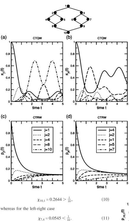
␲jk共t兲 ⬅ 兩␣jk共t兲兩²=兩具j兩Qe^−it␥⌳Q⁻¹兩k典兩². 共9兲 In order to determine numerically the corresponding ei- genvalues and eigenvectors of the matrix A for different graphs we have used the standard software packageMAPLE 7. We start by considering the smaller graph, G = 2, given at the top of Fig. 2. The figures show the transition probabilities for CTQWs and CTRWs starting at the top node 1(left column), which corresponds to the situation described in[10], or at the leftmost node 4(right column). Remarkably, CTQWs start- ing at the top node reach the opposite node 10 very quickly, see Fig. 2(a), much quicker than expected from the CTRW behavior, Fig. 2(c). However, for walks starting at the left- most node 4 and going to the rightmost node 7, the probabili- ties for the CTQWs, Fig. 2(b), and the CTRWs, Fig. 2(d), get to be comparable. Furthermore, the CTQWs’ probabilities,

␲4,4共t兲 and ␲1,1共t兲, of return to the starting node within the time interval depicted in Fig. 2 are much higher if the walks start at the leftmost node 4 of the graph instead of at the top node 1. On the other hand, for CTRWs there is not much difference between starting at the leftmost or at the top node, only that in the first case it just takes a little bit longer to reach a uniform distribution [compare Fig. 2(c) and Fig.

2(d)].

We now extend the time interval to t = 40 and compare the efficiency of the CTQW transport to the CTRW one. In Fig.

3 we plot for the top-bottom and the left-right walks the ratio of the quantum mechanical probabilities␲jk共t兲to the classi- cal ones p_jk共t兲. For top-bottom transport, depicted in Fig.

3(a), the plot turns out to be highly regular, reflecting the high symmetry of the underlying graph in the vertical direc- tion. For left-right transport the plot is less regular. Note the different scaling of the ordinates in the two parts of Fig. 3, which again stresses the preferential role played by the trans- port in top-bottom direction.

In order to discuss what happens at even longer times, we proceed to evaluate for the CTQW the limiting distributions

␹jk given by Eq. (7). For CTRWs the limit is simple: All p_jk共t兲 tend to the same constant, which is the inverse of the total number of nodes in the graph, no matter where the CTRWs start. For the CTQWs, however, this is not the case, as can already be inferred from Figs. 2 and 3. Hence, we compute␹jk for the top-bottom and for the left-right cases separately. Therefore, for the G = 2 graph we compute the eigenvalues and eigenvectors of the respective 10⫻10 ma- trix A and the␹jk by using MAPLE. Having the appropriate eigenvalue matrix⌳and the matrix Q constructed from the orthonormalized eigenvectors we find with Eqs. (7)and(9) and the LinearAlgebra package of MAPLE that for the top- bottom case

FIG. 1. (a)Graph consisting of two Cayley trees of generation G = 3.(b)Horizontal projection of the graph following Ref.[10].(c) Vertical projection of the same graph.(d)Vertical projection of a similar graph, obtained from two Cayley trees of general generation G, indicating the new nodes (clusters) and the d_k (see text for details).

␹10,1= 0.2644⬎₁₀¹, 共10兲 whereas for the left-right case

␹7,4= 0.0545⬍₁₀¹. 共11兲 Thus, the limiting CTRW-probability, ₁₀¹, lies between ␹7,4

and ␹10,1. The top-bottom CTQW is more, the left-right CTQW less efficient than the corresponding CTRW.

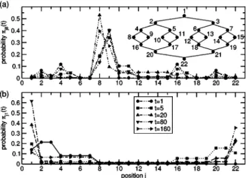
In order to better visualize that the top-bottom and left- right ␹jk are very different, we show in Figs. 4 and 5 the quantum mechanical transition probabilities ␲jk共t兲 for all nodes j when starting(a)at the leftmost node and(b)at the top node; in these figures the time is displayed parametri- cally. Figure 4 is for the G = 3 graph and Fig. 5 for the G

= 2 graph. Now, even for the small graphs considered here, we find differences in the transition probabilities, which clearly depend on the initial node. For the G = 3 graph con- sisting of 22 nodes, the CTQW starting at the top node 1 spreads out rapidly over the whole graph. After a very short time interval, there is a large probability to find the walker at the bottom node 22[see Fig. 4(b)]. However, for the CTQW

FIG. 2. Top: Graph obtained from two Cayley-trees of generation G = 2. Below: Prob- abilities for the CTQW,(a) and(b), and for the CTRW,(c)and (d), to be at node j after time t when starting at time 0 from node 1 or from node 4. Left column,(a)and (c): Starting node is the top node 1. Right column,(b) and (d): Starting node is the leftmost node 4. The time is given in units of the inverse transmission rate␥⁻¹[see text following Eq.(1)].

FIG. 3. Ratios␲jk共t兲/ p_jk共t兲for different directions of propaga- tion,(a) top-bottom walk and(b)left-right walk over time t. See Fig. 2 for units and details.

starting at the leftmost node 8, we have up to times t = 160 a high probability of finding it in the left half of the graph[see Fig. 4(a)]. Therefore, the propagation of the CTQW is strongly dependent on the starting node. For the smaller G

= 2 graph of Fig. 5, which consists of 10 nodes, the effect is similar, but slightly less pronounced.

We illustrate the situation at very long times in Fig. 6, where we display the limiting probabilities␹jkfor the G = 2 and the G = 3 graphs[see Eq.(7)]. For a CTQW starting at the top node 1 the limiting probability distribution has its maxima at the end nodes of the graphs, i.e., at nodes 1 and 10 for G = 2, and at nodes 1 and 22 for G = 3. For a CTQW starting at the leftmost node, k = 4 for G = 2 and k = 8 for G

= 3, the limiting probability distribution shows a strong maximum around the starting node.

Other initial conditions for the CTQW are, indeed, pos- sible, especially when considering the high symmetry of the

underlying graphs. Note that, using for instance the site enu- meration of Fig. 4, a CTQW from node 8 to node 15 is equivalent to a CTQW from, say, node 10 to node 14. The graph’s symmetry suggests to collect groups of such nodes into clusters, while focusing on the transport from left to right. It is then natural to view the nodes 8, 9, 10, and 11 as belonging to the first cluster. The second cluster consists then of the nodes 4, 5, 16, and 17, all of which are directly con- nected by one bond to the nodes of the first cluster. The nodes 2 and 20 of the third cluster are all nodes directly connected by one bond to the nodes of the second cluster, while at the same time not belonging to the first cluster. In general, all the nodes of the共k + 1兲st cluster are connected by one bond to nodes of the kth cluster and at the same time do not belong to the共k − 1兲st cluster.

Let us denote the number of nodes in cluster k by d_k. The transport occurs now from a cluster to the next, by which the original graph gets mapped onto a line in which one new node corresponds to a group of original nodes of the graph.

For a new node at position k苸关2 , G兴 we find that d_k

= 2^G−k+1, the same being true for the mirror node value, i.e., d_k= d_2G+2−k. Note that for the end nodes d₁= d_2G+1= 2^G−1, the same holds for the nodes next to them. Moreover, for the middle node d_G+1= 2.

We now focus on the transport via the states which are totally symmetric, normalized, linear state-combinations for all the original nodes in each cluster. Thus, for the kth cluster, whose sites we denote by n, we have as a new state

兩a_k典= 1

冑

兺

n苸k

兩n典. 共12兲

FIG. 4. Transition probabilities␲jk共t兲 for a CTQW on the G

= 3 graph starting(a)at the leftmost node,␲j8共t兲, and(b)at the top node,␲j1共t兲, for times t = 1, 5, 20, 80, and 160. See Fig. 2 for units and details.

FIG. 5. Transition probability for a CTQW on the G = 2 graph starting at(a) the leftmost node, ␲j4共t兲, and (b) at the top node,

␲j1共t兲, for times t = 1, 5, 20, 80, and 160. See Fig. 2 for units and details.

FIG. 6. Limiting probability␹jk for a CTQW on the(a) G = 2 graph and on the(b)G = 3 graph. Starting points are the top node, k = 1, and the leftmost nodes k = 4 and k = 8, respectively.

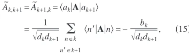
The CTQW is now determined by the new Hamiltonian H˜ =␥^A˜ , where the matrix elements of A˜ are obtained from the new basis states兩a_k典and from the matrix A through

A˜

jk=具a_j兩A兩a_k典. 共13兲 Given the properties of A and the construction of the兩a_k典, Eq. (12), A˜ is a real and symmetrical tridiagonal matrix, which implies a CTQW on a line. The diagonal elements of A˜ are given by

A˜

kk=具a_k兩A兩a_k典= 1 d_kn

兺

苸k n⬘^苸k

具n

⬘

where f_kis the functionality of every node in the kth cluster.

For the sub- and super-diagonal elements of A˜ we find

A˜

k,k+1= A˜

k+1,k=具a_k兩A兩a_k+1典

= 1

冑

兺

n苸k n⬘^苸k+1

具n

⬘

冑

where b_k is the number of bonds between the clusters k and k + 1. Now, except for the ends and the center of the graph, b_kequals the maximum of the pair共d_k, d_k+1兲. Between the central node 共d_G+1= 2兲 and its neighbors 共d_G= d_G+2= 2兲 the number of bonds is b_G= b_G+2= 2. The number of bonds between the end node and its neighbor is b₁= b_2G+1= 2d₁

= 2^G.

For the graph consisting of 22 original nodes the new matrix A˜ is a tridiagonal 7⫻7 matrix, which can be readily diagonalized. The advantage of the procedure is clear: the new matrix A˜ depends on the number of clusters and grows with共2G + 1兲, whereas the full adjacency matrix, A, grows with the total number of nodes in the graph, namely with 共3⫻2^G− 2兲.

From Eq.(12)the transition amplitude between the state 兩a_k典at time 0 and the state兩a_j典at time t is given by

␣

˜_jk共t兲=具a_j兩e^{−iH˜ t}兩a_k典=具a_j兩Q˜ e^{−i␥⌳˜ t}Q˜⁻¹兩a_k典, 共16兲 where⌳˜ is the eigenvalue matrix and Q˜ is the matrix con- structed from the orthonormalized eigenvectors of the new matrix A˜ .

Now the quantum mechanical transition probabilities are given by ␲^˜jk共t兲=兩␣^˜jk共t兲兩². Figure 7(a) shows the transition probabilities for CTQWs over clusters. Remarkably now, and similar to Fig. 4(b), already in rather short periods of time such CTQWs move from one end cluster to the other. The limiting probability distribution, ␹^˜jk, which is depicted in Fig. 7(b), also supports this finding. Note that Fig. 7(b)again reflects the symmetry of the original graph.

In conclusion, we have shown that CTQWs do not neces- sarily perform better than their CTRWs counterparts. By fo- cusing on a particular graph, we have shown that the pen- etration of such a graph by CTQWs can be better or worse than the one by CTRWs, depending on the initial state and on the propagation direction under scrutiny.

Support from the Deutsche Forschungsgemeinschaft (DFG)and the Fonds der Chemischen Industrie is gratefully acknowledged.

[1]J.-P. Bouchaud and A. Georges, Phys. Rep. 195, 127(1990).

[2]R. Albert and A.-L. Barabási, Rev. Mod. Phys. 74, 47 (2002).

[3]S. N. Dorogovtsev and J. F. F. Mendes, Adv. Phys. 51, 1079 (2002).

[4]J. Kempe, Contemp. Phys. 44, 307(2003).

[5]N. van Kampen, Stochastic Processes in Physics and Chemis- try(North-Holland, Amsterdam, 1990).

[6]G. H. Weiss, Aspects and Applications of the Random Walk (North-Holland, Amsterdam, 1994).

[7]Y. Aharonov, L. Davidovich, and N. Zagury, Phys. Rev. A 48, 1687(1993).

[8]E. Farhi and S. Gutmann, Phys. Rev. A 58, 915(1998).

[9]O. Mülken and H. van Beijeren, Phys. Rev. E 69, 046203 (2004).

[10]A. M. Childs, E. Farhi, and S. Gutmann, Quantum Inf.

FIG. 7. (a) Transition probability␲˜_j1共t兲 for a CTQW between different clusters j of the G = 3 graph. The CTQW starts at the first cluster; presented is the situation at times t = 1, 5, 10, 20, 40, 80, and 160. See Fig. 2 for units and details.(b)Limiting probability␹˜_j1for a CTQW starting at the first cluster.

Process. 1, 35(2002).

[11]D. Aharonov, A. Ambainis, J. Kempe, and U. Vazirani, in Proceedings of ACM Symposium on Theory of Computation (STOC’01)(2001), p. 50.

[12]A. Blumen, A. Jurjiu, Th. Koslowski, and C. von Ferber, Phys.

Rev. E 67, 061103(2003).

[13]A. Blumen, C. von Ferber, A. Jurjiu, and Th. Koslowski, Mac- romolecules 37, 638(2004).