Top pair production at the ILC

Top pair production at the ILC

Diploma Thesis of Andreas Moll

Ludwig-Maximilians-Universit¨at Department of Physics

Max-Planck-Institut f¨ ur Physik Supervisor: Prof. Christian Kiesling

December 1, 2008

Zusammenfassung

Das Top-Quark ist einzigartig im Vergleich zu anderen Quarks. Auf Grund seiner kurzen Lebenszeit kann das Top-Quark keine Hadronen oder andere gebundene Zust¨ande bilden und erlaubt somit eine direkte Messung seiner Masse. Durch Strahlungskorrekturen geht die Masse des Top-Quarks in den Elektroschwachen Fit der Higgs-Boson Masse ein und hilft damit die Masse des Higgs-Bosons einzu- grenzen. Das Top-Quark zerf¨allt nahezu ausschließlich in ein W-Boson und ein b-Quark mittels schwacher Wechselwirkung. Das W-Boson kann entweder lep- tonisch in ein Lepton-Neutrino Paar zerfallen oder hadronisch in ein Quark- Antiquark Paar. Diese Arbeit besch¨aftigt sich mit der Erzeugung, Detektor Sim- ulation und Analyse von t t ¯ Paaren am zuk¨unftigen International Linear Collider (ILC). Der ILC ist ein e ⁺ e ⁻ Beschleuniger mit einer Schwerpunktsenergie von

√ s = 500 GeV und einer Luminosit¨at von 500 f b ^{− 1} (innerhalb der ersten vier Jahre).

Es wird eine Methode zur pr¨azisen Messung der invarianten Masse und Breite des Top-Quarks durch direkte Rekonstruktion des Top-Quark Zerfalls vorgestellt.

Dazu werden der vollhadronische und der semileptonische Zerfall von t ¯ t Paaren betrachtet. Im vollhadronischen Zerfall, zerfallen beide W-Bosonen in Quark- Antiquark Paare w¨ahrend im semileptonischen ein W-Boson in ein Quark- Antiquark Paar und das andere W-Boson in ein Lepton und ein Neutrino zerf¨allt.

Zus¨atzlich zu diesen t t ¯ Prozessen werden auch verschiedene Hintergrund Prozesse betrachtet. Die Monte Carlo Produktion der t ¯ t und Hintergrund Ereignisse wur- den f¨ur eine integrierte Luminosit¨at von L = 20 f b ^{− 1} mit der Software PYTHIA durchgef¨uhrt. F¨ur die Simulation des Detektors wurde die Software Mokka und der ILC Detektor LDC’ benutzt, ein ’Zwischendetektor’ Design entwickelt auf dem Weg zur Vereinheitlichung des Europ¨aischen Detektorkonzeptes LDC und des Asiatischen Detektorkonzeptes GLD. Die von der Detektor Simulation er- haltenen Daten werden mit der Rekonstruktions Software Marlin analysiert.

Alle Teilchen werden nach dem Particle Flow Prinzip rekonstruiert und in Jets geb¨undelt. Die Herausforderung liegt in der Auswahl der richtigen Zuordnun- gen von Jets (oder Lepton) zu den W ^± und t ¯ t. Eine Reduktion der Anzahl der m¨oglichen Zuordnungen wird durch Flavour Tagging erreicht. Dabei werden die zwei Jets identifiziert, die aus den b-Quarks hervorgegangen sind. Die folgenden Werte wurden f¨ur die invariante Masse und die Breite des Top-Quarks gefunden:

m t = 175.02 ± 0.17(stat.) GeV und Γ t = 1.67 ± 0.10(stat.) GeV .

i

The top quark is unique among all other quarks. Its short lifetime does not permit the top quark to form top-flavored hadrons or other bound states and allows therefore a direct measurement of its mass. The mass of the top quark enters the electroweak fit for the Higgs boson mass via radiative corrections and helps therefore to constrain the Higgs mass. It decays almost exclusively into a W boson and a b quark via the weak interaction. The W boson can decay either leptonically into a lepton-neutrino pair or hadronically into a quark-antiquark pair. This thesis deals with the production, detector simulation and analysis of t t ¯ pairs at the future International Linear Collider (ILC). The ILC is a e ⁺ e ⁻ collider with a center of mass energy of √

s = 500GeV and a total luminosity of 500f b ^{− 1} within the first four years of operation.

A precise method to measure the invariant mass and width of the top quark from the direct reconstruction of top quark decays is presented considering the fully hadronic decay and the semi-leptonic decay of t t ¯ pairs as signal processes. In the fully hadronic decay both W bosons decay into q q ¯ pairs and in the semi-leptonic decay one W boson decays into a q q ¯ pair and the other W boson into a lepton and a neutrino. In addition to the signal processes, various background processes are also taken into account. The Monte Carlo production of the t t ¯ and background events is performed using the software PYTHIA for an integrated luminosity of L = 20f b ^{− 1} and the simulation of the detector response is carried out with the software Mokka. The ILC detector used for simulation is the LDC’ detector, an intermediate detector designed as a first attempt to merge the European detector concept LDC and the Asian detector concept GLD.

The data obtained from the detector simulation is analyzed within the Marlin software reconstruction framework. All particles are reconstructed according to the particle flow paradigm and clustered into jets. A challenging task is the de- termination of the correct assignment of jets (or lepton) to the W ^± and t ¯ t. The number of possible assignments is reduced by performing Flavour tagging in order to identify the two jets that originated from the b quarks. The values obtained for the invariant mass and width of the top quark are m t = 175.02 ± 0.17(stat.)GeV and Γ _t = 1.67 ± 0.10(stat.)GeV .

ii

Contents

1 Introduction

2 Physics at the ILC

2.1 Fundamental Interactions . . . . 5

2.2 The Standard Model . . . 11

2.3 The top quark. . . 12

2.4 Beyond the Standard Model . . . 19

3 The International Linear Collider 3.1 Motivation for a linear collider . . . 22

3.2 The International Linear Collider . . . 25

3.3 The LDC’ Detector . . . 29

4 Event generation and detector simulation 4.1 Event generation. . . 49

4.2 Detector simulation . . . 52

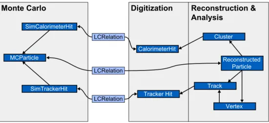
5 Kinematic Reconstruction of Simulated Events 5.1 LCIO . . . 57

5.2 Kinematic Reconstruction of Events with Marlin . . . 60

6 Measurements of the top quark mass 6.1 Jet combinatorics . . . 75

6.2 Background rejection . . . 80

6.3 Kinematic fitting . . . 84

6.4 Final results . . . 88

7 Conclusion and Outlook 8 Appendix 8.1 Discriminating variables distributions for binned likelihood method. . 95

8.2 Likelihood distributions for the 4jet and 6jet channel . . . 102 Acknowledgments

iii

1 Introduction

Since centuries scientists are searching for the ultimate answer to the question about the fundamental structure of matter. To investigate this question a huge number of high precision measurements, paired with enormous achievements in the field of theoretical physics, were performed and are planned for the future.

The LHC at CERN is now the next step in the series of experiments working at the high energy frontier. With a nominal center of mass energy of √

s = 14T eV it runs in the Terascale range and it is therefore expected that the LHC will com- plete the Standard Model of particle physics and look for new physics beyond it. The Standard Model of particle physic describes the current knowledge of ele- mentary particles and their fundamental interactions, except for the gravitational force. The elementary particles are grouped into three generations of fermions, the quarks (up, down, charm, strange, top and bottom) and leptons (e, ν e , µ, ν µ , τ , ν τ ). Additionally, every particle is accompanied by its antiparticle. It is well known that symmetry plays a fundamental role in nature and in particular for the description of interactions between particles. This leads to the theoreti- cal description of interactions as gauge fields and the concept of force mediating particles, called (gauge) bosons. In total there are three interactions described by the Standard Model, which are ordered in increasing strength: the weak, elec- tromagnetic and the strong interaction. For energies around 100 GeV the weak and electromagnetic interaction can be unified to the electroweak interaction. But at these energies the symmetries associated with the electromagnetic and weak interactions are broken. Another problem arises from the fact that the theory requires the gauge bosons to be massless, but in experiments they were found to have mass. Both problems, the electro-weak symmetry breaking and the missing mass of gauge bosons are solved by introducing a new field, the Higgs field, into the theory. The Higgs field acquires a non-vanishing vacuum expectation value, transforming the massless gauge bosons of weak and electromagnetic interactions into massive W ^± , Z ⁰ bosons and a massless photon. It also leads to the prediction of a new massive spin-0 boson, the famous Higgs boson, which explains the origin of fermion masses by the coupling of fermions to the Higgs boson. All particles described by the Standard Model were already discovered in experiments, except the Higgs boson. Thus, the observation of the Higgs boson is the one crucial piece that is still missing. It is expected that the LHC will find the missing piece and therefore complete the Standard Model of particle physics. But various properties and experimental results, like the exclusion of the gravitational force or the obser-

1

vation of dark matter and dark energy in astrophysical experiments, suggest that the Standard Model is not the final theory. One of these theories expanding the Standard Model is for example, the Minimal Supersymmetric Standard Model (MSSM). It predicts that every fermion has a supersymmetric bosonic partner and vice versa. The lightest supersymmetric particle is then a candidate to build the dark matter.

In the picture discussed above the top quark is not particularly distinguished from other quarks. But it turns out that the top quark has some extraordinary features that sets it apart from the other quarks. The short lifetime does not permit the top quark to form top-flavored hadrons or other bound states because it decays before strong interaction effects can influence it. This makes the top quark a perfect tool to study QCD in detail. The most important property of the top quark, in terms of this thesis, is its large mass which is about 172.4 GeV, about 40 times the mass of the next heaviest quark, the b. There are numerous reasons for measuring the top quark mass as precisely as possible, just a few are mentioned here. First of all it is a fundamental parameter of the Standard Model and should therefore be measured as precisely as possible. The top quark mass also enters the electroweak fit for the Higgs boson mass via radiative corrections and helps therefore to constrain the Higgs mass. Since its mass is close to the scale of electroweak symmetry breaking (m _t ∼ Λ _SB ), the top quark might also play an active role there. In the MSSM it puts constraints on the parameters of the scalar top sector and therefore allows sensitive tests of the MSSM by comparing predictions with direct observations.

The physics program at the LHC contains a top physics program with the precise measurement of the top mass being a main goal. But there is another collider currently under discussion, which is even better suited to measure the top mass with a high precision, the International Linear Collider (ILC). The ILC is a linear e ⁺ e ⁻ collider with a center of mass energy of √

s = 500GeV . Its main advantages compared to the LHC are the point-like elementary colliding particles, which leads to a well defined initial state of the collision, its tunable center of mass energy which allows for advanced analysis methods like threshold scans and the possibility to adjust the polarization of the beams. In addition, due to the electro- weakly interacting initial state, the expected background from Standard Model processes is moderate.

This thesis describes the simulation and full reconstruction of t ¯ t decays at the fu-

ture linear collider ILC. The top quark almost exclusively decays into a W boson

and a b quark. The W boson can decay either leptonically into a lepton-neutrino

pair or hadronically into a quark-antiquark pair. Therefore, depending on the

decays of the W bosons the t ¯ t events can be classified into three channels. In

the fully hadronic channel, both W bosons decay hadronically and the final state

topology is t ¯ t → (bq q)(¯ ¯ bq q). In the semi leptonic channel one of the W bosons ¯

3 decays leptonically and the other one hadronically, leading to the final state topol- ogy t ¯ t → (bq q)(¯ ¯ blν). The last channel is the dileptonic channel, where both W bosons decay leptonically t t ¯ → (blν)(¯ blν). In this thesis the fully hadronic and semi-leptonic channels were simulated and reconstructed. The analysis concen- trates on the precise measurement of invariant mass and width of the top quark from the direct reconstruction of top quark decays. In contrast to complementary top mass measurement methods like threshold scans, the method presented in this thesis does not need the collider to run in any special mode. The top mass can be directly measured from data taken from the collider operating at 500 GeV.

Similar studies have been done above the t t ¯ threshold, e.g. S.V. Chekanov and V.L. Morgunov studied the reconstruction of top quarks in the fully hadronic decay channel for the TESLA detector and obtained

m t = 176.08 ± 0.39(stat.)GeV

and Stefan Kasselmann estimated the invariant mass for the CMS detector at the LHC. He found

m t = 174.3 ± 0.22(stat.)GeV

In the simulation study presented in this thesis and in both similar studies a top mass of 175 GeV was assumed. But none of the similar studies achieved an unbiased measurement, which means that the reconstructed mass with the statistical error is equal to the input mass. Thus, their systematic error must be large.

Naturally the question arises, which precision for the measurement of the invariant top mass can be achieved at the ILC ? In the following chapters, this thesis try to answer this question.

In chapter 2, a short introduction into particle physics is given. The theories that led to the Standard Model and the Standard Model itself are explained and the measurement of top quark properties is motivated.

Chapter 3 provides an overview of the future International Linear Collider (ILC) and discusses the detector concept LDC’. The requirements on the detector design and the basic concepts, like particle flow analysis, that were developed to fulfill the given requirements are presented. The various subdetectors are explained and their parameters summarized.

The discussion of the top quark pair analysis starts in chapter 4 with the Monte

Carlo production of signal and background events. Standard software package

were used to produce Monte Carlo data for different final states in e ⁺ e ⁻ collisions.

The Monte Carlo data was then put into a full detector simulation software, in order to simulate the detector response of the LDC’ detector. The simulation process and strategy is presented in this chapter, too.

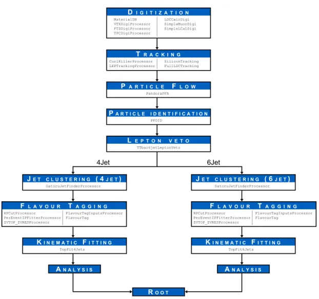
Chapter 5 addresses the full reconstruction of the simulated events from chapter 3. The reconstruction chain is presented and the various reconstruction steps and algorithms like tracking, particle flow, jet clustering and flavour tagging are explained. Special emphasis is put on the reconstruction and selection algorithms.

Chapter 6 presents the final steps in the top mass measurement. The methods that were developed for reconstructing the top quarks from the reconstructed particles and for the rejection of background events are discussed, finally the result for the invariant mass and width of the top quark, together with their errors, is given.

Chapter 7 concludes the top mass measurement which is presented in this thesis

and gives an outlook onto further studies.

2 Physics at the ILC

In this chapter the present status of particle physics is briefly reviewed focusing on the top quark in the Standard Model. The interest in a precise measurement of the top quark mass is motivated.

2.1 Fundamental Interactions

At the end of the nineteenth century many physics thought that all basic physical laws were already discovered, and what was left to be done is just to refine their details. It was assumed that the laws of Newton (classical mechanics) and the Maxwell equations (classical electromagnetism) are sufficient to describe all present and future physic phenomena.

Planck, Lorentz, Einstein, Bohr, de Broglie, Schr¨odinger, Heisenberg, Dirac and others showed that this assumption was wrong. They introduced revolutionary new concepts and theories, most importantly special relativity and quantum me- chanics, to explain ’obscure’ experimental results.

Fig. 2.1: Plaque, outside the Cavendish laboratory in Cambridge, commemorates Sir Joseph Thomson’s discovery of the electron.

In terms of particle physics, important experimental milestones that mark the beginning of this field are, among others, the discovery of the electron in 1897 by

5

J.J. Thomson (see fig. 2.1) [1] and the scattering of alpha-particles by a thin gold foil in 1911 done by Geiger, Marsden and Rutherford [2].

About 100 years and a lot of experimental results later, it is believed that the constituents of matter are fermions with spin ¹ ₂ , called ’particles’ within this thesis. Classically, the forces acting between particles are mediated by a field.

However, from the standpoint of modern quantum mechanics, the interaction between particles are mediated by the exchange of virtual particles having spin 1, the gauge bosons which are also called ’force carriers’. The strength of an interaction is measured by a coupling constant.

The four basic forces, ordered in increasing strength, are [3]:

• Gravitational force

• Electromagnetic force

• Weak force

• Strong force

The first force, the gravitational force, is very small in all known atomic and sub- atomic processes (about 10 ²⁵ times less than the strength of the weak force) and therefore its effect is negligible in particle physics. Only the weak, electromagnetic and strong force play an important role in this physics field.

To explain observed particles and interactions or predict new ones, physicists build theories using fundamental concepts like special relativity, quantum me- chanics, mathematical group theory and symmetry considerations. A very impor- tant property that is required in constructing a quantum-mechanical theory of particles which are interacting in a given manner with a field, is called local gauge invariance [4]. This property requires that the constructed theory is invariant un- der a gauge transformation that has one or more parameters varying with the space-time coordinates. For example, the three basic theories, QED, QCD and Weak, building the present fundamental model of particle physics the ’Standard Model’ [3] (see section 2.2), have this property.

2.1.1 Quantum Electrodynamics

Classical electromagnetism defines the electric field E and magnetic field B which

obey Maxwell’s equations [5]. Planck, Einstein and Compton showed with their

work on the spectrum of black-body radiation, the photoelectric effect and the

scattering of photons by electrons that the electromagnetic field is quantized, with

the quantum of the field being the photon. It was Dirac who discovered in 1928 a

first-order linear differential equation which describes the quantum mechanics of

2.1 Fundamental Interactions 7 point-like, spin ¹ ₂ particles, completely consistent with special relativity. Apply- ing this equation to electrons, he predicted an electrically positive version of the electron, now known as the positron, which was discovered 3 years later in cosmic radiation [6]. The combined theory, describing the interaction of the charged Dirac field with the quantized electromagnetic field, is called quantum electrodynamics (QED). It was finished in 1950 by Feynman, Schwinger and Tomonaga who re- ceived the Nobel Prize for Physics for their work on QED in 1965. The associated mathematical symmetry group is constructed by applying a simple local gauge invariance. This leads to a field that has all the properties of the electromagnetic field, with the strength of the interaction g em determined by a constant of the gauge transformation. The strength g em is identified as the charge of the parti- cle. This symmetry group is called U(1) and predicts one massless gauge boson associated with the field. This gauge boson, mediating the interaction between charged particles, is the well-known photon.

2.1.2 Quantum Chromodynamics

The scattering experiment by Rutherford [2] established the existence of the atomic nucleus and showed its linear dimension to be of the order of 2 to 7 · 10 ^{− 15} m.

Over the last century, high energy accelerators (e.g. HERA) and the precise mea- surement of physical quantities like the cross-section in scattering experiments, extended the scale of human knowledge down to 10 ^{− 18} m. Especially the measure- ment of the cross-sections for deep inelastic scattering of electrons by nucleons, led to the present understanding of the structure of nucleons. Nucleons are bound systems of smaller particles, called quarks and antiquarks. They are bound by a force, called strong force due to its strength. It is approximately 10 ³⁸ times higher than the gravitational force (determined by the values of the corresponding cou- pling constants). The strong force is mediated by virtual particles called gluons.

Fig. 2.2: The quark structure of a proton: two up quarks and one down quark.

The theory of the quark-gluon interaction is called quantum chromodynamics

(QCD). There are in total six types of quarks (+ their antiquarks): up, down,

charm, strange, top and bottom. The different types of quarks are also called the

quark flavours. Apart from electrical charge, quarks and gluons carry a special

charge, called color charge or in short color [7]. There are three kinds of colors:

’red’, ’green’ and ’blue’. Quarks are always forming color-neutral (the colors are mixing to ’white’) composite particles, called hadrons. Two famous examples are the two nucleons: neutron and proton. The proton consists of two up and one down quark (see fig. 2.2), the neutron of one up and two down quarks. To distinguish the hadrons from particles that do not experience the strong force, like the electron or the muon, these particles form an independent group of particles called the leptons.

The associated symmetry group of QCD is SU(3). It predicts 8 massless spin-1 gauge bosons, the mentioned gluons with the strength of the coupling (labeled g s ) determined by the color of the particles. Unlike QED, the gauge boson in QCD, the gluon, carries the interaction charge and can therefore interact with other QCD gauge bosons (gluons).

Quarks and gluons are not directly observable, they are always confined within colorless states. By separating two colored objects, for example q q ¯ (see fig. 2.3), a flux tube of self-interacting gluons is formed, the color field, and it would take an infinite amount of energy to separate both objects. This property is called color confinement.

q q

Fig. 2.3: Separating a q and a q ¯ leads to the formation of a flux tube of self- interacting gluons.

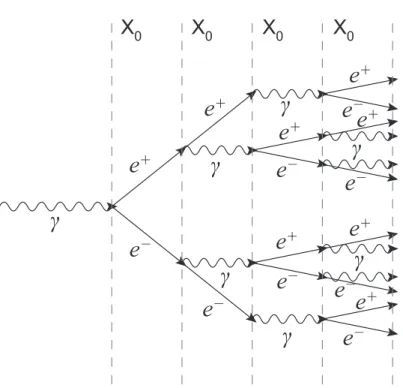
By separating the quarks, the energy stored in the color field starts to increase, until E stored > 2m q . Then, new q q ¯ pairs can be created [8]. In the end, these pairs are forced by color confinement to build colorless particles, hadrons (see fig. 2.4), shaping an higher level object: narrowly collimated jets of hadrons.

This process of starting out with quarks and ending up with jets is called hadronization. Fig. 2.5 illustrates the hadronization of the process e ⁺ e ⁻ → q q. ¯ The hadrons in a jet produced from q( q) follow the direction of the original q(¯ ¯ q).

Consequently, the process e ⁺ e ⁻ → q q ¯ is observed as a pair of back-to-back jets of hadrons.

2.1.3 The Weak Interaction

The weak interaction is very different, compared to the interactions discussed

above. The interaction is mediated by three massive gauge bosons called W ⁺ ,

2.1 Fundamental Interactions 9

q q

q q

q q q

q

Fig. 2.4: If the energy stored in the color field is larger than 2m q , new q q ¯ pairs can be created which finally build hadrons.

̟ ⁺

̟ ⁺ ̟

K ⁺

p

̟ ^–

̟ ⁺

̟ ^–

̟ ^–

̟

̟ ⁺

̟ ^–

̟

̟

̟ ⁺

̟ ^–

̟

̟ ⁺

̟

K ⁺

̟ ^–

̟ ^–

e ⁺ e ^–

q

q e ⁺

e ^–

γ

q q

Fig. 2.5: The hadronization of the process e ⁺ e ⁻ → q q. The final state is observed ¯

as a pair of back-to-back jets of hadrons. The time development of the

hadronization process is illustrated in the lower part.

W ⁻ , Z ⁰ and couples to all quark and lepton doublets. Additionally, the weak interaction can change the flavour of particles and is therefore responsible for the majority of particle decays. A historical example for the manifestation of the weak interaction is the β ⁻ decay:

n → p + e ⁻ + ¯ ν _e

It describes the conversion of a bound neutron into a bound proton, emitting an electron and a neutrino.

The weak interaction is called weak, because its strength is effectively quite small.

It is approximately 10 ⁵ times less than the strength of the electromagnetic force (determined by the values of the corresponding coupling constants). It is char- acterized by ’long’ lifetimes (compared to hadronic processes) and small cross- sections. From a mathematical point of view, the weak interaction is governed by the symmetry group SU(2).

2.1.4 Electroweak unification

The electromagnetic and weak interactions can be unified in the framework of SU (2) ⊗ U (1) gauge interaction. The unified interaction is called ’electroweak interaction’. The work on formulating a single, locally gauge invariant electroweak theory was done by Glashow, Weinberg and Salam [9, 10, 11, 12] who received the Nobel Prize in 1979.

The symmetry group of this theory requires 4 massless spin-1 bosons as carriers of the interaction: One triplet, consisting of W ⁺ , W ⁻ , W ⁰ (W _µ ⁱ , i = 1, 2, 3) and a neutral singlet called B ⁰ (B _µ ). From experimental observations [13], it is known that the three gauge bosons mediating the weak interaction are W ⁺ ,W ⁻ , Z ⁰ and the gauge boson mediating the electromagnetic interaction is the photon (γ). In the electroweak theory, Z ⁰ and γ are therefore created as a linear combination of the two electrically neutral components W ⁰ and B ⁰ . Written in terms of the neutral fields W _µ ³ , B µ , the photon field A µ and the Z boson field Z µ , the linear combination is [14]:

A µ = B µ cos θ w + W _µ ³ sin θ w

Z _µ = − B _µ sin θ _w + W _µ ³ cos θ _w

The angle θ w is called Weinberg angle and parametrizes this mixing. But there

is a serious problem. The mixing is only valid for massless gauge bosons. In

experiments the bosons W ⁺ , W ⁻ and Z ⁰ are found to have mass and any naive

way to introduce masses would violate the underlying gauge symmetry.

2.2 The Standard Model 11 In summary, this leads to two fundamental questions:

• Why is the electroweak interaction broken into the electromagnetic and the weak interaction for energies below 1TeV ?

• Is there a mechanism that gives mass to the bosons W ⁺ ,W ⁻ , Z ⁰ and leaves the photon massless ?

2.1.5 The Higgs boson

These problems are solved by introducing a new field, the Higgs field [15, 16], and one accompanying massive spin-0 boson, the famous Higgs boson. The Higgs field has a non-zero vacuum expectation value. This property is responsible for spontaneously breaking the electroweak gauge symmetry into the electromagnetic and the weak one, which is referred to as the Higgs mechanism [17], named after P.W. Higgs, who discovered it. The Higgs mechanism is also responsible to give mass to the gauge bosons W ⁺ , W ⁻ and Z ⁰ . Since the Higgs coupling strength is related to the mass of the particles, the photon remains massless. The masses of fermions can also be explained by the Higgs theory. While the gauge bosons get their masses via spontaneous symmetry breaking, the fermions acquire mass via coupling to the Higgs boson.

2.2 The Standard Model

Joining together the three described theories, QED+Weak+QCD, into one single model, leads to the Standard model of particle physics. It describes the currently known elementary particles and their interactions. Fig. 2.6 shows an overview of the particles and interactions of the Standard Model.

The elementary particles are grouped into three generations of spin ¹ ₂ fermions,

the quarks (up, down), (charm, strange) and (top, bottom) and leptons (e, ν e ), (µ,

ν µ ) and (τ, ν τ ). Additionally, every particle is accompanied by its antiparticle. The

first generation alone suffices to build all ’visible’ matter. The heavier particles

from the second and third generation are unstable and decay into the lighter

particles of the first generation. The Standard Model describes three interactions,

mediated by spin 1 bosons. The electromagnetic interaction, mediated by the

massless photon (see section 2.1.1), the weak force mediated by three massive

bosons W ⁺ ,W ⁻ and Z ⁰ (see section 2.1.3) and the strong interaction mediated

by eight colored gluons (see section 2.1.2). The spin 0 Higgs boson introduced in

section 2.1.5 is the last ingredient of the Standard Model and the only one which

as not yet been observed.From a mathematical point of view, the standard model

is a gauge theory with the combined symmetry group SU(3) ⊗ SU(2) ⊗ U (1).

Fig. 2.6: The Standard Model of elementary particles consists of elementary par- ticles divided into three generations of leptons and quarks, and gauge bosons as force carriers [18].

Due to color confinement, quarks and gluons are not directly observable. But the existence of quarks was shown in hadron spectroscopy, deep inelastic lepton scattering by nucleons [19], production of hadrons in e ⁺ e ⁻ annihilation and other experiments. All leptons have been observed directly, either by observation of the free particle itself (e ⁻ and µ ⁻ ) [20, 21] or of its decay products (τ ⁻ ) [22] or by observation of collisions caused by the particle (ν e , ν µ and ν τ ) [23, 24]. The last lepton to be discovered was the τ neutrino. It was announced on 21. July 2000 that the τ neutrino was observed at the DONuT experiment [24] at Fermilab.

Since the existence of the antifermions is certain and confirmed in most cases, it is the Higgs boson that remains to be found. Therefore, its discovery is the prime target of upcoming experiments like the Large Hadron Collider (LHC) [25].

2.3 The top quark

2.3.1 The top quark in the Standard Model

The mass of the Higgs boson is a free parameter in the Standard Model and there-

fore not given by the theory. However, experimental and theoretical constraints

can be applied to limit the possible mass range. This is necessary, because the

2.3 The top quark 13 Higgs boson production modes and decay channels depend on its mass. A lower limit of m H > 114.4GeV at a 95% confidence level is given by the measurements of all four LEP experiments [26]. An upper limit for the Higgs boson mass can be derived from the theoretical side. The theory requires unitarity to be conserved in high-energy scattering of gauge bosons, leading to a theoretical upper limit of m H < 700GeV [27]. The upper limit can be improved further, with the top quark mass and the W boson mass playing a major role.

The mass of the W is given by the electroweak theory [28, 29, 30, 31]:

m W =

v u

u t πα em

√ 2G F

! 1 sin θ W

(2.1)

where α _em = ^g ₄

_π ≈ 137 ¹ [32] is the electromagnetic coupling constant, θ _W the Weinberg angle and G F = 1.166 · 10 ^{− 5} GeV ^{− 2} [33, 34] the Fermi coupling constant.

The mass of the Z ⁰ boson is [35, 36]:

m Z = m W

cos θ W

(2.2) Hence, if any three of α em , G F , m W , m Z , sin θ W are known, the other two param- eters can be predicted. For example, measurements at LEP obtained the following values for m Z [13] and sin ² θ W [37, 38, 39]:

m Z = 91.1875 ± 0.0021GeV sin ² θ W = 0.23154 ± 0.00016 According to (2.2) the expected value for m W is:

m W = 79.946 ± 0.008GeV

But the measurement obtained [40]:

m W = 80.398 ± 0.025GeV

This difference is due to the equations (2.1) (2.2), only describing the lowest order terms of the W mass formula. Higher order corrections that include terms from virtual loops (see fig. 2.7), have to be taken into account, too [14]:

m W = m W

· 1

√ 1 − ∆r (2.3)

W

+

t

b

+

W H ⁰

Fig. 2.7: Feynman diagrams for loop corrections to the W boson mass The correction term ∆r is sensitive to contributions from the top quark and the Higgs boson mass m H :

∆r ≃ 1 − α _em

α(m Z ) − 3G _F m ² _t 8 √

2π ² 1 tan ² θ W

+ 11G _F m ² _Z cos ² θ _W 12 √

2π ² ln m _H m Z

(2.4) with α(m Z ) = 127.92 at Z0 pole (M S scheme) due to the running of α em . Inverting (2.3) and knowing the values of the top quark mass and the W boson mass from experiments, a constraint on the Higgs boson mass can be obtained.

This was done by the LEP Electroweak Working Group [40] taking into account, among other things, published measurements of the W boson mass [40] and the top quark mass [41]:

m W = 80.398 ± 0.025 GeV

m top = 172.4 ± 0.7(stat) ± 1.0(syst.) GeV

From these inputs they compute an upper limit on the Higgs boson mass of m H <

144GeV (m H < 182GeV if the lower limit is included) at the 95% confidence level.

A comparison of the indirect measurements (dashed contour) and the direct mea- surements (solid contour) of m W and m t is shown in fig. 2.8. An indirect measure- ment means that the values for m _W and m _t are obtained from Standard Model parameters like the Z mass, the Weinberg angle θ W etc. A direct measurement however, reveals the W and top masses from direct reconstruction. Fig. 2.8 also shows the Standard Model predictions for the Higgs boson masses between 114 GeV and 1000 GeV. The indirect and direct measurements of m W and m t are in good agreement and prefer a low value of the Higgs boson mass.

The constraints on the Higgs boson mass, imposed by the top quark mass, is a first hint that the top quark is unique among all other quarks.

One of the extraordinary features of the top quark refers to its lifetime. The

shape of the energy spectrum of an isolated state of finite lifetime is Lorentzian

and shown in fig. 2.9. The full width at half height is called Γ. ^Γ ₂ is then the

2.3 The top quark 15

80.3 80.4 80.5

150 175 200

m _H [ GeV ]

114 300 1000

m _t [ GeV ]

m W [ GeV ] ^{68 % CL}

∆α LEP1 and SLD

LEP2 and Tevatron (prel.)

July 2008

Fig. 2.8: The top quark and the W boson mass constrain the mass of the Higgs particle. The ellipses represent mass limits obtained from combined mea- surements at LEP, SLD and Tevatron. The green are indicates the pre- dicted Higgs mass within the Standard Model [42].

E ₀ +Γ/2

E ₀ ^Energy

E nt ri es

E ₀ −Γ/2 σ ₀ /2

σ ₀

Fig. 2.9: The Lorentzian line shape. This is the shape of the energy spectrum of

an isolated state of finite lifetime. The full width at half height Γ is the

energy uncertainty.

energy uncertainty. With ∆t being the uncertainty of lifetime, the uncertainty in the total energy (∆E) is given by:

∆E∆t ∼ = ¯ h

2 (2.5)

In a decaying state the uncertainty ∆t is equal to the mean life (τ) of that state.

With ∆E = ^Γ ₂ the mean life τ is:

τ = h ¯

Γ (2.6)

According to [43], the top quark width, as predicted in the Standard Model, is:

Γ top = G F m ³ _top 8π √

2 1 − m ² _W m ² _top

! 2

1 + 2 m ² _W m ² _top

! "

1 − 2α s

3π 2π ²

3 − 5 2

!#

(2.7)

The width increases with the third power of the mass of the top quark. For a top mass of ≈ 175GeV the width is ≈ 1.5GeV , which is approximately an order of magnitude larger than the strong interaction scale (Λ QCD ≈ 200M eV ). The lifetime of the top quark computes, according to (2.6) with ¯ h = 6.582 · 10 ^{− 22} M eV s and Γ top = 1.5GeV to:

τ top = 4.4 · 10 ^{− 25} s

The short lifetime does not permit the top quark to form top-flavored hadrons or other bound states [44] which need a typical ’formation time’ given by the time scale of the strong interaction O(10 ^{− 23} s). It therefore decays as a ’free quark’.

This is a unique feature of the top quark among all other quarks and makes it a perfect tool to study QCD in detail.

Another property that sets the top quark apart from other quarks, is its extraor- dinarily large mass. The next heaviest quark, the b, has a mass of only 4.2GeV . This high mass is the reason why the top quark was discovered just over a decade ago [45, 46]. Since its mass is close to the scale of electroweak symmetry breaking (m t ∼ Λ SB ), the top quark might also play an active role there.

In summary it may be said that the unique features of the top quark suggest

a detailed study of its properties, in particular the determination of its mass as

precisely as possible.

2.3 The top quark 17

2.3.2 Top quark decay

The weak interaction is responsible for the decay of the top quark. It decays, by changing its flavour, into a W boson and one of three possible quarks: s, d or b

t → W s t → W d t → W b

In general, the strength of (flavour changing) weak decays is summarized in a uni- tary matrix, called Cabibbo-Kobayashi-Maskawa matrix (CKM Matrix, V _CKM ) [47, 48]. Technically, it describes the creation of a weak eigenstate from mass eigenstates:



 



d ^′ s ^′ b ^′



 



| {z }

W eak eigenstates

=



 



V ud V us V ub

V cd V cs V cb

V td V ts V tb



 



| {z }

V



 



d s b



 



| {z }

M ass eigenstates

The probability of a transition from one quark q 1 to another quark q 2 is propor- tional to | V q

q

| ² . Unfortunately, the matrix elements are not predicted by the Standard Model and have to be determined from experiments. Applying a global fit to all available measurements and imposing Standard Model constraints, the CKM Matrix is found to be (uncertainties excluded) [49]:

| V CKM | =



 



0.9738 0.2272 0.0039 0.2271 0.9729 0.0421 0.0081 0.0416 0.9991



 



From the CKM Matrix the probabilities for the decay of the top quark to a s,d or b quark can be estimated:

| V td | ² = 6.62 · 10 ^{− 5} | V ts | ² = 1.73 · 10 ^{− 3} | V tb | ² = 0.99

The value for | V tb | ² is close to unity, thus the top quark almost exclusively decays into a W boson and a b quark. The following discussion will therefore concentrate on this decay channel using a t ¯ t pair as the inital state. The Feynman diagram for the process e ⁺ e ⁻ → t t ¯ → (W ⁺ b)(W ⁻ ¯ b) is shown in fig. 2.10.

The created W bosons can decay either leptonically into a lepton-neutrino pair

or hadronically into a quark-antiquark pair. Within the Standard Model, the

branching fractions of the W bosons depend on the six matrix elements | V q

q

| of

the CKM Matrix not involving the top quark. In the following classification of t ¯ t

e ⁺ e ^–

Z ^* / γ ^*

t t

b b

W ^–

W ⁺

Fig. 2.10: Feynman diagram of the decay of a t ¯ t pair into a W ⁺ ,W ⁻ ,b and ¯ b decays, it will be assumed that all W boson decays have equal branching fractions which is an approximation often found in literature. The possible W boson decay modes are illustrated in fig. 2.11.

The decay channels of a t t ¯ pair can be classified, based on the decay of both W bosons, into three different groups:

Fully hadronic channel

t t ¯ → (W ⁺ b)(W ⁻ ¯ b) → (q qb)(q ¯ q ¯ ¯ b)

In this channel, both W bosons decay into quark-antiquark (q¯ q) pairs. In fig. 2.11 this channel is represented by the red area and happens approximately 36/81 = 44.4% of the time. The final state consists of 6 quarks, which hadronize and are therefore observed as 6 jets.

Semi-leptonic channel

t ¯ t → (W ⁺ b)(W ⁻ ¯ b) → (q¯ qb)(lν ¯ b)

This channel is characterized by the decay of one W boson into a quark-antiquark (q q) pair and the other W boson decaying into a lepton (l ¯ = electron, muon, tau) with the associated neutrino (ν). Approximately 2 · (18/81) = 44.4% of t ¯ t pairs decay semileptonically, represented by the orange areas in fig. 2.11. In the final state of this channel 4 jets and a lepton are observed. The associated neutrino escapes undetected, but its presence is revealed by the momentum it carries away.

Momentum conservation requires the final state to have a total momentum of

zero. The difference in momentum between zero and the summed momenta of

jets and lepton is associated as the ’missing’ momentum with the neutrino. The

2.4 Beyond the Standard Model 19

(bb) (gg) (rr) (bb) (gg) (rr)

cs cs cs ud ud ud τ

ν

μ

ν

e

ν

(W

b)(W

b) tt

W

(bb) (gg) (rr) (bb) (gg) (rr)

cs cs cs ud ud ud τ

ν

μ

ν

e

ν

W

Fig. 2.11: W Boson decay modes of the t ¯ t system [50].

energy of the neutrino is calculated from energy conservation. Thus, the full four- vector information of the undetected neutrino is available in this decay channel.

Dileptonic channel

t ¯ t → (W ⁺ b)(W ⁻ ¯ b) → (l ⁺ νb)(l ⁻ ν ¯ ¯ b)

Both W bosons decay into leptons (l = electrons, muons, taus) and the associ- ated neutrinos (ν). Only approximately 9/81 = 11.1% of t t ¯ decays fall into this category, represented by the green area in fig. 2.11. In the final state 2 jets and 2 leptons are observed. Since two neutrinos escape undetected, there is not enough information to calculate the four-vectors of the decay products, as opposed to the semi-leptonic channel.

2.4 Beyond the Standard Model

All experimental observations discussed so far are consistent with the Standard Model. But it turns out that it is not a complete theory. The following properties suggest that it must be part of a more comprehensive theory:

1. The actual strengths of the coupling constants g em (QED), g s (QCD) and

the Weinberg angle θ W (Weak) are not given by the present theory.

2. It does not predict either the existence of three generations or the mixing of quark generations.

3. The masses of the fermions are parameters which have to be experimentally determined and cannot be predicted.

4. Gravity is not included in the standard model. It is not yet clear how to combine quantum field theory with general relativity.

5. Data from astrophysical experiments [51] show that only about 5% of the total energy in the universe is of baryonic origin (mostly protons), covered in the Standard Model. About 25% of the total energy consists of the not yet discovered dark matter and the missing 70% are assigned to the so called dark energy. Thus, the Standard Model is not able to explain 95% of the total energy in the universe and has to be extended.

The Terascale

"Grand Unification"

Planck Scale

Big Bang Electroweak Unification

Electromagnetic Force

Weak Nuclear Force Strong Nuclear Force Gravitation

Time (s) Energy (TEV) 10

10

10

1 10

10

10

10

10

10

10

10

10

10

10

10

1 10

10

10

10

10

Fig. 2.12: Unification of all four forces in a Grand Unification Theory [52].

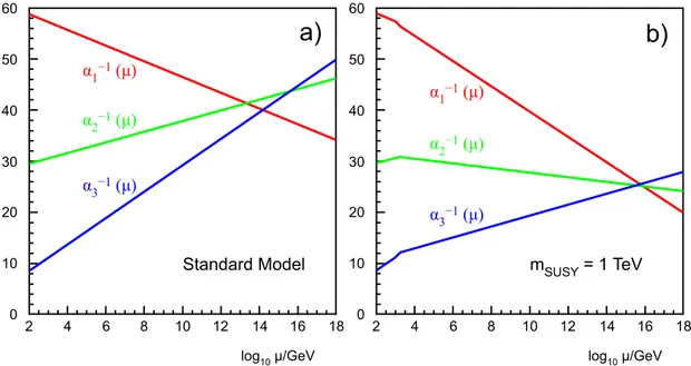
Another problem arises from the fact that the coupling constants (like g _em ,g _s ,) are not constant at all, they vary with momentum transfer. Therefore the coupling constants are also called ’running constants’. These running constants lead to a ’problem’. Fig. 2.12 indicates that for very high energies the interactions and therefore the gauge couplings should merge to one single interaction. But with the coupling constants running, as predicted by the Standard Model, the gauge couplings do not meet at a single point, shown in fig. 2.13a).

It turns out that an extension to the Standard Model called Supersymmetry

solves this problem by allowing the unifaction of gauge couplings at a single point

(see fig. 2.13b)). The Minimal Supersymmetric extension of the Standard Model

2.4 Beyond the Standard Model 21 (MSSM) [53, 54, 55] predicts that every fermion has a supersymmetric bosonic partner and vice versa. Apart from unifying the gauge couplings, Supersymmetry also provides supersymmetric particles that might be candidates for the dark matter. Such a particle is for example the Lightest supersymmetric particle (LSP).

2 4 6 8 10 12 14 16 18

0 10 20 30 40 50 60

log

μ/GeV

Standard Model

a)

α ₃ ⁻¹ (μ) α ₂ ⁻¹ (μ) α ₁ ⁻¹ (μ)

2 4 6 8 10 12 14 16 18

0 10 20 30 40 50 60

log

μ/GeV

m _SUSY = 1 TeV α ₃ ⁻¹ (μ)

α ₂ ⁻¹ (μ) α ₁ ⁻¹ (μ)

b)

Fig. 2.13: The three coupling constants within the Standard Model a) and the MSSM b) .

There are many other extensions to the Standard Model, not mentioned here that

try to provide answers to the open questions of particle physics. But nevertheless,

the Standard Model is able to make quantitative predictions about the behavior

of particles at energies up to the mass of the W and Z ( ≈ 100GeV ). Beyond this

energy, new physics is to be expected probably at the TeV scale and with the

LHC at CERN, a machine is now available that will reach those energy ranges.

3.1 Motivation for a linear collider

High energy accelerators proved to be one of the most essential tools for physicists to learn about phenomena at scales far from our direct experience. Basically, high energy accelerators convert matter into energy and via collisions of the energetic beam particles back to matter again, according to Einsteins famous equation E = mc ² . The Standard Model, discussed in chapter 2, is a triumph of theoretical predictions and high energy accelerators physics. But the open questions now demand accelerators reaching into the TeV energy range (Terascale).

3.1.1 Synergy of Hadron and Lepton colliders

The Large Hadron Collider (LHC), started in September 2008 at CERN, is such a machine. Protons are accelerated in a circular tunnel with a circumference of 27 kilometers. They form two beams, traveling in opposite direction which collide with a center of mass energy of 14 TeV. As the name suggests, the LHC is a so-called Hadron collider, compared to another type of collider, called Lepton collider which accelerates and scatters leptons. A typical example would be an electron-positron collider.

The complementarity of both accelerator types has already proven in the past to be essential for the understanding of high energy phenomena. Hadron colliders are at the energy frontier and are used as discovery machines, whereas Lepton colliders operate at lower energies and allow very precise measurements. Two examples should emphasize the importance of the synergy created by both collider types:

• The experimental verification of the Standard Model would not have been possible without the Hadron collider Tevatron (operating at 1.8 TeV) and the lepton colliders LEP (90-200 GeV) and SLC. The LEP, for example, allowed comprehensive tests of the coupling structure of the fundamental fermions and gauge bosons at the level of quantum corrections.

• The mass of the top quark was predicted by precision measurements made

22

3.1 Motivation for a linear collider 23 by the Lepton colliders LEP and SLC. The Hadron collider Tevatron finally discovered the particle in 1995. Using results from both colliders, it was possible to constrain the mass of the Higgs boson to be below 200 GeV at a confidence level of 95% [40] within the Standard Model (see 2.3.1).

With the LHC running, the question about a complementary lepton collider nat- urally arises. The basic requirements needed for a comprehensive physics program at a future Lepton collider are the following: It should have a minimal center of mass energy of ≃ 2 · m top ≈ 400GeV with the option for an upgrade to ≈ 1T eV , the possibility to adjust the center of mass energy and to achieve a luminosity of 300 to 500f b ^{− 1} per year.

The main disadvantage of a hadron collider is the rather difficult determination of the partons which actually collide and their real collision energy. The uncertainty of the initial states makes the interpretation of the collected data challenging. On the other hand, a lepton collider has a well defined initial state and all the energy of a colliding particle is carried by a single constituent. Therefore the full center of mass energy is used for the collision of particles.

3.1.2 The ILC - a complementary accelerator to the LHC

The answer of the particle physics community to the demand for a Lepton collider is the International Linear Collider (ILC). The ILC is a future electron-positron collider with a center of mass energy of √

s = 500GeV . The center of mass energy range, available for physics runs, ranges from √

s = 200GeV to √

s = 500GeV . The beam energy can be adjusted for mass threshold scans and additionally the electron and positron beams can be polarized. For the future, an option for an upgrade of the center of mass energy to √

s = 1T eV is planned. The total luminosity of the collider is 500f b ^{− 1} within the first four years of operation. These basic parameters, together with the high precision measurements possible at the ILC, make it the perfect complementary Lepton collider for the LHC.

The precise tasks of the ILC depend on the upcoming discoveries at the LHC, but in general the future workspaces for the International Linear Collider are two-fold.

On the one hand, any new particles discovered by the LHC that are kinematicaly

accessible at ILC energies, can be studied in great detail. Properties like quantum

numbers, decays, production modes, cross-sections and coupling constants are

directly accessible. On the other hand, the ILC is also able to have a deeper look

into multi-TeV regions, even if these regions are far above the direct kinematicaly

reach of the ILC. This capability relies on the fact that the ILC is able to carry out

high precision measurements. By measuring differential cross-sections, quantum

level effects arising from virtual particles in loops can be studied (see section

2.3.1). This technique of exploring new particles and phenomena outside the

range of a collider has already been successfully exploited at LEP and SLC. For example, in 1994, LEP measurements of m Z gave a prediction that the top quark mass was about m t = 175 ± 20GeV , which was measured later in 1994 by the Tevatron collider to be m t = 174.1 ± 5.4GeV .

The high precision measurements at the ILC are possible mainly due to the following reasons:

• The colliding particles (electron, positron) are point-like elementary parti- cles, leading to a well defined initial state of the collision.

• The center of mass energy of the ILC is tunable, allowing for advanced analysis methods like threshold scans.

• The polarization of both beams (electron and positron beam) can be ad- justed. This makes detailed analysis of the helicity structure of processes possible.

• The expected background from Standard Model processes is moderate, due to the simple, electro-weakly interacting initial state.

• Advanced detector design and reconstruction algorithms allow for precise measurements.

The discovery of the Higgs boson and the study of the Higgs mechanism is one of the main missions of the LHC. Concerning the Higgs particle there are three possible outcomes. First of all, the Higgs particle is found at the LHC and is consistent with the Standard Model. This means, the Higgs boson is ’light’, with a mass < 200GeV (see section 2.3.1). The ILC can then verify that the Higgs mechanism works exactly the way it is predicted by the theory. In addition, the high precision measurements allow for a detailed search for possible nonstandard properties of this mechanism. The second possible outcome of the LHC is that the Higgs particle is found, but heavier than predicted. It would then be inconsistent with data from precision electro-weak measurements. Therefore, the tasks of the ILC would be to verify the discovery of the LHC and to apply precision measure- ments to find the reason for this inconsistency. The third possibility is that no Higgs particle is discovered. In this case the ILC has to make sure that the LHC hasn’t missed anything. Again high precision measurements could be applied to get a hint of undiscovered phenomena that are responsible for the electro-weak symmetry breaking and for the origin of mass.

The second discovery field for the LHC is ’Physics beyond the Standard Model’,

e.g. Supersymmetry. If Supersymmetry is realized in nature and at a mass scale

of order 1 TeV, the LHC will find it. The ILC, for example, with its tunable

center of mass energy, can then precisely measure the masses of the color-neutral

superpartners by threshold scans, if they are accessible at ILC energies.

3.2 The International Linear Collider 25 Another application of this technique at the ILC is the measurement of parame- ters of the top quark, for example the invariant mass and width. As mentioned above, the ILC allows the tuning of the beam energy. A threshold scan works by varying the beam energy and measuring the cross-section for a specific process.

Since the cross-section of the top quark process e ⁺ e ⁻ → t ¯ t depends, among other things, on m top and Γ top , these parameters can be extracted from the measured cross-section.

3.2 The International Linear Collider

The answer of the particle physics community to the demand for a complementary lepton collider to the LHC is the International Linear Collider (ILC). In this chapter the basic working principles of the ILC as well as the requirements for a detector in order to reach the physics goals of the ILC are discussed.

3.2.1 Linear vs Circular

Main Linac

Damping Rings

Main Linac 31 km

e

e

e ⁻

Positrons

Electrons

Undulator

Detectors Electron

Source

Beam Delivery System

Fig. 3.1: Basic Layout of the International Linear Collider [56].

The basic layout of the ILC is shown in fig. 3.1. It consists of two linear accelerator parts, the left one for electrons and the right one for positrons. The interaction area, including the interaction point where the particles collide, is located in the center.

The reason for building a linear accelerator instead of a circular machine is mainly

due to the effect of synchrotron radiation. In a circular accelerator, the electrons

and positrons are kept in orbit by bending magnets. They therefore feel the cen-

tripetal force mediated by the bending magnets and are accelerated towards the

center of the accelerator. According to classical electrodynamics, an accelerated

charged particle radiates energy. If this happens for a particle following a curved

path or orbit, the radiation is called synchrotron radiation. The radiated energy

is lost for the particle and has to be replaced by the accelerator.

The relativistic formula for the radiated power P for a single electron is (in SI units) [5]:

P = 2Ke ² γ ⁴ a ²

3c ³ (3.1)

P = 2Ke ² γ ⁴ v ⁴

3c ³ r ² (3.2)

with the Coulomb’s constant K = 8.99 · 10 ^{9 N m} _C

, e the charge of the electron, c the speed of light, γ the Lorentz factor, a = ^v _r

the centripetal acceleration in a circular orbit, v the velocity of the electron and r the radius of the accelerator.

The loss of energy per orbit is then given by

∆E = P 2πr

v = 4πKe ² γ ⁴ v ³

3c ³ r (3.3)

For highly relativistic particles (v ∼ c), the term γ ⁴ dominates the loss rate.

Since the particle energy is

E = γmc ²

the loss of energy by synchrotron radiation scales as the fourth power of the particle energy. The consequences are dramatic: The LEP experiment, the pre- decessor collider of the LHC, accelerated electrons and positrons and achieved an energy of about 100 GeV. The planned ILC is going to accelerate the same particles to an energy only 2.5 times higher. This would mean the energy loss by synchrotron radiation is 2.5 ⁴ ≈ 39 times higher. To cope with the radiation loss, one would have to increase the size of the rings, since the radiation loss is inversely proportional to the radius of the ring. To have approximately the same amount of radiation loss in a circular ILC as in the LEP experiment, the circum- ference would have to be increased from 27 km to more than 670 km ! Even if a linear accelerator means that the whole machine has to be filled with expensive acceleration structures compared to only a small part in a circular accelerator, the absence of synchrotron radiation really pays off.

3.2.2 The accelerator

The two linear accelerators (see fig. 3.1) at the ILC have in total a length of about

30 kilometers. To produce the electrons for the accelerator a 2ns laser pulse is

3.2 The International Linear Collider 27 fired on a target and knocks out electrons. Using normal-conducting structures, bunches of electrons are created and pre-accelerated to 76 MeV. A supercon- ducting linear accelerator pushes the electrons to 5 GeV, before superconducting solenoids rotate their spin into the vertical. Then the electron bunches are injected into the electron damping ring.

Positrons are created by sending the high energy (multi-GeV) electrons through an undulator. In an undulator dipole magnets are arranged in a periodic structur (see fig. 3.2) which force the electrons to undergo oscillations and to radiate synchrotron radiation. While the electrons return to the main accelerator, the photons created in the undulator hit a titanium-alloy target and create a beam of electron-positron pairs. The positrons are collected and accelerated to 5 GeV.

Superconducting solenoids rotate the spin vector of the positrons into the vertical, before they are injected into the positron damping ring.

S N

S N

S N N S

N S

N S

Fig. 3.2: The basic structure of an undulator. Periodically arranged magnets force electrons to undergo oscillations and to radiate synchrotron radiation.

The damping rings have a circumference of 6.7 km and are used to squeeze the transverse dimensions of the electrons/positrons bunches further and to store them before they are sent to the main linear accelerators. The squeezing process is done with a device called wiggler [57][58], which is similar to an undulator, except the fact that the energy spectrum of the emitted photons is much broader.

On their way from the damping rings to the starting point of the linear accel- erators, the polarization of the beams is rotated from the vertical to the angle required at the interaction point and the particles are accelerated from 5 GeV to 15 GeV. The particles then enter the main, 12 km long, linear accelerators, which accelerate them from 15 GeV to the the final beam energy of 250 GeV.

Each linear accelerator is composed of many cryomodules, each of them consist

of eight or nine superconducting cavities, encapsulated in a vacuum vessel. The

cryomodules are operated at a temperature of 2K, cooled by superfluid helium,

to make the cavities superconducting.