Variables Selection in Observational and Experimental Studies

Variables Selection

in Observational and Experimental Studies

by

Joachim Kunert and Claus Weihs

Fachbereich Statistik, Universität Dortmund

March 2000

Abstract

This paper discusses whether differences in the data structure of observational and experimental studies should lead to different strategies for variable selection.

On the one hand, it is argued that outliers in the predictor variables have to be treated differently in the two kinds of studies. In experimental studies this results in philosophical problems with the applicability of cross validation. On the other hand, it is shown, however, that a well designed experiment might lead to a factor structure very appropriate for cross validation, namely a certain balance in the observations together with orthogonality of the factors. This might be the reason why in practice cross validation has proven to be a valuable tool for variable selection also in experimental studies. In contrast, however, it is shown that variables selection based on cross validation is not appropriate for saturated orthogonal designs.

After this fundamental argumentation, we illustrate by a number of examples that the same methods for variable selection can be successfully applied in observational as well as experimental studies.

Keywords

variables selection, stepwise regression, cross validation, principal components, screening, optimization

1.Introduction

Variables selection methods are examples for the use of cross validation in observational as well as in experimental studies (see, e.g. SAS-Stat User’s Guide, PROC REG and PROC RSREG). This paper describes both ways of application, and compares them. In section 2 we introduce variables selection by means of ‘greedy’ stepwise forward selection (cp. Weihs (1993) and Weihs and Jessenberger (1999)). Section 3 discusses the use of cross validation in experimental studies from a theoretical viewpoint and gives conditions favorable and unfavorable for variable selection by means of cross validation. In sections 4 and 5 for observational studies as well as for experimental studies, we will present examples for the application of variable selection with cross validation.

2. Greedy variables selection

In order to identify those factors which mainly influence a target variable in a linear model y = Xβ+ ε, one can build the linear model for the target by, e.g., successively including the influential factors. This is done by identifying first that factor with the biggest effect on the target, then the factor with the biggest additional effect, etc. until no ‘essential’ improvement of model fit can be observed.

Such a method is called forward selection or stepwise regression with forward selection if the ‘least squares criterion’ is used to judge the effect size. If a factor once chosen is always kept in the model, the method is called ‘greedy’ forward selection.

Even if there are less observations n than possibly influential factors K, then stepwise regression allows to study whether the target can be modeled adequately with B < n−1 factors.

Essential for the functionality of such a method is the choice of an appropriate measure for (the actually reached) model adequacy, here expressed by the predictive power. One possibility for measuring predictive power is cross validation. A special version of cross validation is leave one out, where each observation of the sample is left out once individually, n regressions with n−1 observations each are carried out, and each of the left out observations

each observation one gets an oblique prediction. The differences of these to the true observations are used to define the predictive power.

Predictive power based on leave one out

Assuming that the current model of the target Y has K influential factors, the predictive power corresponding to a target Y is defined as

( )

R : 1 RSS

y y

cv

2 cv

i 2 i 1

= − n

−

∑

i 1

= n

∑

and the ˆ_i := y_i − yˆ_i,cv, i = 1, ..., n, are the prediction errors, yi is the i^th observation of the target, ^yˆi,cv^:=^xi^T ˆ

( )

is the i^th row of the design matrix, and βˆ

( )

In what follows R2cv will be used as the performance measure in greedy forward selection.

Stepwise regression with greedy forward selection

In stepwise regression with greedy forward selection first that factor is chosen out of the possibly influential factors, which maximizes R2cv in a model with (possibly an) increment and one factor only. Then another factor is chosen, the addition of which to the model increases R2cv most, etc. until R2cv does not improve anymore.

Before the application of this method we discuss its mathematical background.

3. Cross validation

3.1 Cross validation in observational studies

The philosophical background of cross validation (in the authors’ opinion) works as follows:

Assume we have n (K+L)-dimensional vectors of observations (xi, yi), i = 1, ..., n. We assume that these are a random sample of independent identically distributed (K+L)-dimensional variables with unknown joint distribution P^X,Y.

Assume that for an (n+1)^stobservation we have as yet only observed the part xn+1 and we want to use this to make a good prediction for yn+1. We assume that (xn+1,yn+1) also has the distribution P^X,Y. The prediction yˆ_n+1 will be some function f of the observed xn+1,

ˆ_n+1

y = f(xn+1), and the so-called prediction rule f will be determined by regressing y on x in the set (x1,y1), ..., (xn,yn).

To see how well this prediction works, we could use several independent observations (xn+r, y_n+r), r = 1, ..., m, where we would calculate the prediction yˆ_n+r and compare this to y_n+r (train-and-test method). The mean deviance

∑

= + − +

m

r

r n r

m yn y

1

1 ˆ 2 gives an estimate of

E( Y−Yˆ ²), the performance of the prediction. In practice, however, if we had these additional observations, we would like to include them in the learning sample, to get a better prediction rule f.

Cross validation with the leave one out technique provides another unbiased estimate of E( Y−Yˆ ²), which does not need the extra-observations. We omit one observation (x_s,y_s) from the sample (x1,y1), ..., (xn,yn), then we calculate the prediction formula from the remaining n-1 observations and we use this formula to calculate a prediction yˆ_s,cv for the one observation that has been omitted. Then y_s−yˆ_s,cv ² is an estimate of E(

ˆ 2

Y

Y− ). Repeating this for every s, we get the cross validated estimate

∑

= −

n

s

cv s

n ys y

1

2 ,

1 ˆ , which is equal to RSScv / n considered in section 2 in the case of one target Y only.

If we want to compare several models for prediction, then we might want to select the one for which

∑

= n −

s

cv s s

n y y

1

2 ,

1 ˆ is smallest. Note that this destroys the validity of

∑

= n −

s

cv s s

n y y

1

2 ,

1 ˆ

2

basically the same predictive power, such that

∑

= −

n

s

cv s

n ys y

1

2 ,

1 ˆ has basically the same distribution for each of the predictors. Consequently, since we select the one model with the minimal

∑

= −

n

s

cv s

n ys y

1

2 ,

1 ˆ , we underestimate E(

ˆ 2

Y

Y− ). Therefore,

∑

= −

n

s

cv s

n ys y

1

2 ,

1 ˆ is a

good means to select an appropriate model, but it then gives a too optimistic view of the performance of the model which is actually chosen.

3.2 Cross validation and designed experiments

The situation is very different, however, if a designed experiment is carried out. With a designed experiment, the set {x1, ..., xn} is deliberately chosen. Therefore, the (xi, yi) are not identically distributed. Additionally, the new observation (xn+1, yn+1) is not just another observation with the same distribution, but the point xn+1 for which we want to predict y is a fixed point of interest. In most cases it is a point where we did not observe during the experiment.

Example 1 (Simulation):

We take an artificial example to show, how cross-validation can be misleading for a designed experiment. Assume that we have observed a one-dimensional x at points x₁= 0.1, x₂= 0.2, x₃

= 0.3, x4= 0.4, x5= 0.5, x6 = 0.6, x7= 10. Further assume that the conditional distribution of a one-dimensional y given x is the normal distribution with expectation 10+x and variance 1.

If the data were derived from an observational study, then there is a good argument that the observation 7 might be an outlier. If the data were derived from an experiment, then we have designed x₇to be different from the other x_i. Therefore there is no reason why this observation should be less reliable than the others.

Assuming the model described above, we simulated 10,000 data sets with the given xi, i=1,...,7, and corresponding yi. There are two simple models which we might use for prediction. The first model does not take account of the x,

(M1) y =µ+ε ,

whereas the second model uses x, (M2) y =µ+βx +ε .

We know from the way how we have simulated the data that (M2) is the correct model. If the data were observations from a true experiment or a true observational study, then we would

not know which is the right model. We would have to decide from the data which model appears more adequate.

We compare two methods for deciding between the models. The first method is cross validation. For each of (M1) and (M2) we calculate

∑

= −

n

s

cv s

n ys y

1

2 ,

1 ( ˆ ) . We select the model for which this quantity is smaller. The second method is significance testing. From the data, we test whether βis significantly different from 0. If it is, then we use model (M2) for prediction, if not, we use (M1).

For each of the 10,000 simulated data sets, we performed both methods to decide between the two models. We chose x* = 0.3 as the point at which we wanted to predict. Then we calculated the predictions from both models, and compared how well the prediction fitted to 10+x*, the conditional expectation of y at x*.

We found that among the 10,000 data sets, in all cases ß was significant, while cross- validation correctly decided for the regression-model (M2) only in 3,497 of the 10,000 experiments. So there were 3,497 cases where significance testing and cross-validation decided for the same model. In the remaining 6,503 cases, there were 213 when the simpler model (M1) chosen by cross validation gave better prediction, while there were 6,290 cases when model (M2) chosen by significance testing gave better predictions in x*.

Things were even more extreme if for the same 10,000 simulated data sets we chose to predict at x* = 5. Then the prediction from the regression model (M2) was better in all 10,000 cases.

Therefore, significance testing chose the better model in 6,503 cases, while cross-validation never chose a model which led to a better prediction than the one chosen by significance testing.

The results in Example 1 need some comments. It is clear that the poor performance of the cross validation is due to the fact that there is just one single x_i which is far away from the others. With an observational study, we would usually not have just one observation for which the x-value is far away from the others. If we had, then we might decide that observation 7 is an outlier and not use this observation for prediction at all. Therefore, the prediction from model (M1) would fit much better to observations 1 to 6 (and give much better prediction for x*=0.3). With an observational study which observes x_i’s in the range between 0 and 1, we would usually not want to make predictions for x* = 5.

The example seems to show that cross validation is not appropriate for designed experiments.

This, however, is only part of the story. Had the experiment been properly designed then cross validation would not produce such results.

To get an impression of how cross validation performs with designed experiments, some theoretical considerations will be helpful. Assume that we have a matrix X =

[

]

ε + γ + β

= X x* y

where βis a (K+1)-dimensional vector and γ a constant, while εis a random vector, such that E(ε) = 0 and Cov(ε) =σ² In. We consider RSS_cv when the model

ε + β

= X y

is assumed, i.e. when the factor associated with γis neglected in the model.

We start with some definitions. Let ω^⊥(X)=I_n−X(X^TX)⁻¹X^T , d_i =1−x_i^T(X^TX)⁻¹x_i the i^th diagonal element of ω^⊥( X), and D=diag(d₁,...,d_n). Let yˆ= X(X^TX)⁻¹X^Ty, the least squares estimate for y from the assumed model, and yˆ_cv =[yˆ_1,cv,...,yˆ_n,cv]^T the vector of predictions of y from leave one out cross validation.

With these definitions we have (see e.g. Cook and Weisberg, 1982, p. 33) that

ˆ) ˆ D ¹(y y y

y− _cv = ⁻ − .

As y−yˆ=ω^⊥(X)y and as y = Xβ+x*γ+ε, it follows that ε

ω + γ ω

=

− yˆ D^{−1 ⊥}(X)x* D^{−1 ⊥}(X)

y _cv .

Therefore,

)

* )(

( )

( )

* E(

) ˆ ( ) ˆ E(

)

E(RSS_cv = y− y_cv ^T y− y_cv = ε+x γ ^Tω^⊥ X D⁻²ω^⊥ X ε+x γ .

Due to the fact that E(ε) = 0, we get

*) ) ( )

(

*

² ) ( )

( E(

)

E(RSS_cv = ε^Tω^⊥ X D⁻²ω^⊥ X ε+γ x ^T ω^⊥ X D⁻²ω^⊥ X x . (1)

The first term in (1) can be transformed to

(

)

tr ) ) ( )

(

E(ε^Tω^⊥ X D⁻²ω^⊥ X ε = ω^⊥ X D⁻²ω^⊥ X εε^T

( ) ( ) _∑

=

⊥

−

⊥

−

⊥ = =

= ⁿ

i i

n D X d

I X D

X

1 2

2 1

²

² ) ( tr

² ) ( )

(

trω ω σ ω σ σ ,

because di is the i^th diagonal element of ω^⊥( X) and because D^-2 = diag( 1/d₁²,...,1/d_n²).

In the situation that γ = 0, i.e. when the fitted model is appropriate, then it is desirable that E(RSS_cv) is as small as possible. Using that

∑

1

² / 1

1

1

1 = − −

−

≥

∑

∑

n d n

n

i n

i i

with equality holding if all diare equal. Hence, in the special instance that γ = 0 and that all di

are equal, we have

1

² ² )

E( = − −

K n

RSS_cv σ n .

In this case, we can see an advantage of RSScv compared to RSS, the usual sum of squares for errors: since n² / (n - K -1) is increasing in K, we have E(RSScv) increasing if some additional irrelevant parameters are added to the fitted model.

In the case γ ≠ 0, we consider the second term in (1). Defining

[

]

∑

⊥

−

⊥ = ⁿ

i

i i

T X D X x a d

x

1 2 2

2 ( ) * ² /

) (

*

² ω ω γ

γ .

Note that

∑

So, if all d_iare equal, it is true that

* ) *

1 (

² ² 1

² ²

* ) ( ) *

1 (

² ² 1

² ² )

E( _{2 2} x x

K n

n K

n x n

X K x

n n K

n

RSS_cv n ^{T T}

− γ −

− + σ −

≤

− ω γ −

− + σ −

= ^⊥

with equality if x* is orthogonal to the factors in the fitted model.

If we compare this to the corresponding formula for the case that x* is included in the fitted model

2

² ²

~ )

E( = − −

K n S n

S

R _cv σ ,

then we see that ~ ) E( ) E(RSS_cv ≤ RSS_cv if

* ) *

1 (

² ² 1

² ² 2

² ² ₂ x x

K n

n K

n n K

n

n T

− + −

−

≤ −

−

− σ γ

σ .

Some algebra shows that this is equivalent to

* 1 *

² 1 2

² 1 x x

K n K

n

T

−

≤ −

−

− γ

σ .

So the performance of the refined model with x* included in comparison to the simpler model depends on the size of γ²x*^T x* compared to σ².

However, it should be noted that this holds only if

a) for both models all diare equal, and

b) x* is orthogonal to the columns of X, i.e. to the factors contained in the simpler model.

Note that condition a) formulates a sort of balance in the observations since it demands that all observations xiT

have the same norm corresponding to some Mahalanobis distance.

The poor performance of cross validation in Example 1 can be explained easily: in the finer model the di were highly dissimilar. In fact, d7 = 0.002, while di = 0.2 for the other observations. In contrast, all di would have been equal for the linear regression model, if half of the x_i had been +a or -a each, for some appropriate number a. The second term of (1) then is maximised if a is as large as possible (for constant effect γ). Interestingly, this is the D- optimal linear regression design (see, e.g. Pukelsheim, 1993, p. 57).

There are famous designs for which conditions a) and b) are fulfilled. The fractional factorial designs build a class of designs with the desired structure. With a fractional factorial design for every submodel with K ≤ n-2 factors or interactions we have X^TX=n I_K+1. It follows that

n K x X X

x^T_i ( ^T )⁻¹ _i =( +1)/ , independent of i, because each x_i consists of K+1 elements which are either +1 or -1. Additionally, we have for each additional factor or interaction that x* is orthogonal to every column of X. If we restrict attention to main effects only, then the same properties are fulfilled for Plackett-Burman-Designs.

For variable selection properties a) and b) have a very important impact. They imply that the second term of formula (1) is proportional to γ²⋅x*^Tx*, where γ is the effect of the factor not included in the fitted model. Therefore, the size of RSS_cv is reduced the most if the factor with the largest |γ| x*^T x* is included in the model. If then, as in fractional factorial and Plackett-Burman designs, all x*^Tx* are equal, this is the factor with largest |γ|. Therefore, for such designs greedy variables selection can be based on the absolute value of the estimates of the unknown coefficients corresponding to the possibly influential factors. Hence, it is not necessary to determine R²_cv for all possible factors individually to identify the next factor to be included in the model. Instead, this factor can be fixed just by inspection of the coefficients determined by estimating the model where all factors are included. R²cv is only used as a stop criterion, i.e. to determine the model size.

Unfortunately, inspection of the stopping rule shows that conditions a) and b) also imply that for saturated orthogonal designs like Plackett-Burman designs greedy variables selection is always choosing the maximum model. This can be seen as follows.

Let us assume n > K+2 for the moment. Then, from condition a) it follows for a model with K factors that

ˆ) 1( ˆ)

ˆ ¹( y y

K n y n y D y

y _cv −

−

= −

−

=

− ⁻ .

Therefore,

K cv

K RSS

K n RSS n

, 1

−

= − ,

where RSSK,cv and RSSK stand for the residual sum of squares after K factors have been included in the model. The stopping rule would stop variables selection iff crossvalidated R² is smaller after the (K+1)^th step than after the K^th step, i.e. iff inclusion of one more variable would decrease performance. This can be shown to generate a contradiction as follows.

2 , 2

,

1cv Kcv

K R

R ₊ <

is equivalent to

cv K cv

K RSS

RSS _+1, > _,

in the case of all diequal because of the above relationship of RSScv and RSS is equivalent to

K

K RSS

n-K- RSS n-K-

1 2

1 >

+ .

If SSC_K+1 := γ²K+1 SS_K+1 is defined as the contribution of factor (K+1) to the overall sum of squares of the target, then for orthogonal factors these contributions are summing up to the overall sum of squares, and thus

K K

K

K RSS SSC RSS

RSS n-K-1

2 - K - n

1

1 = − ₊ >

+

which is obviously equivalent to

) 1

1

( − − ₊

> K

K n K SSC

RSS .

This leads, however, to a contradiction for a saturated orthogonal design. In such a design there are exactly (n-K-1) factors remaining as candidates for inclusion in the model with contributions at most that high as for the factor to be chosen in step (K+1) since this is factor with maximum RSScvand thus RSS of the factors remained for selection. Moreover, ultimately RSS will be zero because of the orthogonality of the factors, and therefore RSSK has to be equal to the sum of the contributions of all remaining (n-K-1) factors. This is obviously not possible if the last inequality is valid.

The only case to be discussed is when K = n-2 , i.e. K+1 = n-1 and thus only one factor is remaining. In this case, RSS_K+1 and thus RSS_K+1,cv has to be zero, and thus R²_cv takes its maximum value, and also this factor is chosen, if it generates a nonzero contribution. Thus, in saturated orthogonal designs the stopping rule is only eliminating factors with zero contribution.

In what follows examples of variables selection in observational and experimental studies are discussed, in particular with respect to conditions a) and b).

4. Observational Studies

In the following section we give two examples of applications of the variables selection method from section 2 which illustrate two very different conditions for the application of such a method in observational studies. In both examples, the method is applied to principal components since they are typical intermediate outcomes of observational studies.

4.1 Interpretation of Principal Components

In principal component analysis, variables selection can be applied to simplify and interpret

minimum number of original variables. This yields illuminating and surprising results (cp.

Weihs and Jessenberger, 1999).

Indeed, principal components Zk, k= 1, ..., K, are weighted sums Xgk of the (mean centered) original variables. The question is now, can we easily judge the importance of an original variable directly by means of the size of the corresponding weights in gk, called loadings, or do we actually have to apply something like the complicated variables selection method above?

The first idea is to order the original variables directly by the size of their loadings to judge their importance for the corresponding principal component. Unfortunately, this can only be justified if the involved values of the observed variables are similar in size and if these variables are uncorrelated. Indeed, the i^th observation x_ij of the j^th variable influences the i^th observation of the k^th principal component only via its so-called contribution

jk j

ij x g

x − )⋅

( _{, wherexj} is the mean of the observations of the j^th variable, and gjk is the loading of the j^th variable on the k^th principal component. Moreover, even a large contribution cannot be taken as an indicator that the corresponding principal component cannot be

‘represented’ without the corresponding observed variable because of the correlation of the observed variables. Indeed, it may be possible to approximate the principal component adequately without a variable with a large contribution since variables highly correlated with that variable can replace it nearly completely. Note the relationship to the conditions for the simplified variables selection technique indicated in the end of section 3.2. In that section the same size of the observations and the orthogonality of the variables were also identified to be sufficient conditions to base variables selection only on effect sizes, i.e. on loadings in the present section.

Thus, a method deciding directly by means of the loadings about the importance of an original variable for the representation of a principal component is not in sight. However, the variables selection method in section 2 could be applied, e.g., to the scores of one principal component as the target in order to identify a simple model based on the observed variables which guarantees good prediction of scores. It will be illustrated by the next example, however, that with such a method the influence of highly correlated variables on the target can also not

really be separated, but that the number of relevant original variables identified by variables selection can be much smaller than expected from loadings inspection.

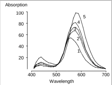
Example 2 (Characteristic wavelengths, cp. Lawton and Sylvester, 1971): For five produced batches of a dyestuff, a characteristic absorption spectrum was measured at the wavelengths 410 nm to 700 nm in steps of 10 nm. Thus, the data set consists of five observations of 30 variables. In this special example, the observed variables can be graphically illustrated very easily since the wavelengths have a natural ordering. Indeed, the five dyestuff batches can be displayed in a diagram with wavelength at the x-axis and absorption at the y-axis (s. Figure 1). Each dyestuff batch then corresponds to one absorption curve called spectrum.

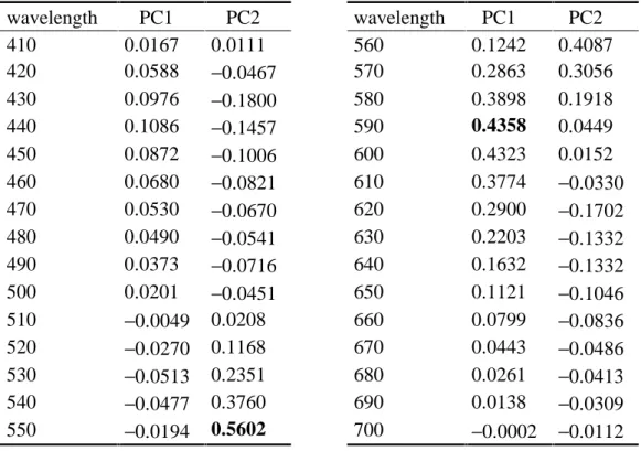
In order to characterize the differences between the five batches in a simple way with minimum loss of information, the first two principal components (PC1 and PC2) of the 30 wavelengths were calculated based on the empirical covariance matrix of the observed 30 variables, which represent 96% of the variation in the data. These characteristics are weighted sums of all the wavelengths (s. Table 1). Here, the absolute value of the weights (i.e. of the loadings) is maximum for 590 nm with PC1 and for 550 nm with PC2 so that these wavelengths can be seen as the first candidates to be responsible for the variation in the data, i.e. between the batches. In other words, one might suspect that the five batches are most different in these wavelengths.

400 500 600 700

Wavelength 20

40 60 80 100 Absorption

1 5 4

2 3

Figure 1: Absorption spectra

Table 1: Loadings of the first two principal components in the dyestuff example wavelength PC1 PC2 wavelength PC1 PC2

410 0.0167 0.0111 560 0.1242 0.4087

420 0.0588 −0.0467 570 0.2863 0.3056

430 0.0976 −0.1800 580 0.3898 0.1918

440 0.1086 −0.1457 590 0.4358 0.0449

450 0.0872 −0.1006 600 0.4323 0.0152

460 0.0680 −0.0821 610 0.3774 −0.0330

470 0.0530 −0.0670 620 0.2900 −0.1702

480 0.0490 −0.0541 630 0.2203 −0.1332

490 0.0373 −0.0716 640 0.1632 −0.1332

500 0.0201 −0.0451 650 0.1121 −0.1046

510 −0.0049 0.0208 660 0.0799 −0.0836

520 −0.0270 0.1168 670 0.0443 −0.0486

530 −0.0513 0.2351 680 0.0261 −0.0413

540 −0.0477 0.3760 690 0.0138 −0.0309

550 −0.0194 0.5602 700 −0.0002 −0.0112

And indeed, in Figure 1 one may confirm that the wavelengths 550 nm and 590 nm are important for the distinction of the batches. In particular, the batches appear to be most distinctly different in wavelengths around 600 nm, and in wavelength 550 nm the observations of the batches happen to have a different order than around 600 nm.

Now, stepwise regression with greedy forward selection is applied. Astonishing enough, this method leads to the conclusion that both the first two principal components can be nearly perfectly represented by only one wavelength each (s. Table 2), which could not be expected by the size of the loadings.

Table 2: Interpretation of principal components

PC1 PC2

wavelength 590 nm 550 nm

R2cv 1.0 0.85

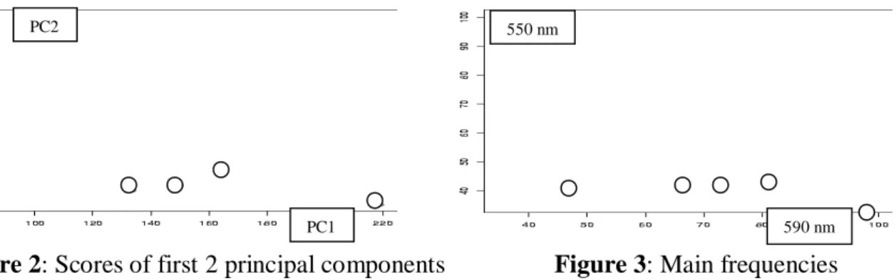
Note that besides wavelength 590 nm also wavelenghts 600 nm and 610 nm produced R2cv near to 1.0. This result may be interpreted as that the influence of highly correlated variables on the target cannot really be separated with the proposed variables selection method. But in any case, the two wavelengths 590 nm and 550 nm appear to be sufficient to characterize the differences between the five batches. This is supported by the similarity of the projections of the five batches in figures 2 and 3.

Figure 2: Scores of first 2 principal components Figure 3: Main frequencies

Finally note that predictive power is tentatively overestimated by the reported R²cv with the described model selection method since R²cv was used heavily for model selection as well as for the estimation of predictive power (cp. section 3.1).

4.2 Principal Components Regression

In principal components regression, the conditions for applying variables selection methods are somewhat different. The idea is to select those principal components with the strongest linear influence on some target variable. Principal components as influential factors have the big advantage that their effect is not changing when other principal components are added to or eliminated from the model since principal components are uncorrelated, and thus orthogonal to each other. Since the originally observed variables are generally correlated, such a statement is not true for models with a target in dependence of the originally observed variables. Thus, the conditions for variables selection methods are much better in principal components regression than in interpretation of principal components above. Indeed, the selection method appears to be much simpler.

Principal components regression

Let X be the mean centered maximum rank data matrix of K observed variables, let y be the mean centered data vector of a target variable, and Z the scores matrix of the principal components based on the data X.

The model of principal component regression has then the form: Y = Zβ+ε, where βis the vector of unknown coefficients, and εthe vector of model errors.

Then, since Z has maximum column rank, the least squares estimate of βhas the

form:

( )

1) (n

y y Z

Z Z Z ¹

−

′

=Λ

′

′

= ^{− −1}

β^ˆ , where Λ is a diagonal matrix with

PC1 PC2

590 nm 550 nm

0 ) r(

aˆ v 1)

r(

aˆ

11=v ≥ ≥λ = >

λ Z K _KK Zk . The k^thcoefficient β^ˆ_k has thus the form:

( )

ˆ

Zk r a v 1 n

y z_k

k −

= ′

β , and

) 1 ) r(

aˆ ˆ v r(

aˆ

v = −

Z n

2 k

k

β σ is independent of k, where zk

is the k^th column of Z, i.e. the scores of the k^th principal component. Thus, the coefficient of the k^th principal component actually does not depend on the other principal components. And moreover, standardizing the principal components zk

by their standard deviation, i.e. introducing ~ / vaˆr( )

k k

k z Z

z = , leads to estimated coefficients with constant variance.

Note that the contribution of a standardized principal component to a target is thus determined by an estimated coefficient with constant variance. Therefore, in order to select the component with the biggest contribution, we can concentrate on the absolute value of these

‘standardized’ coefficients. Using R²cv as the predictive power criterion for variables selection, this leads to the following method for the construction of a prediction model for the target Y based on observed influential factors X₁, ..., X_Kby means of principal components.

Variables selection in principal components regression

Carry out a full principal component analysis on X, i.e. generate all K principal components. Then, the coefficient of each principal component in a model for a certain target variable Y can be estimated individually, i.e. ignoring the other principal components. Therefore, variables selection just selects the components one by one by the size of the absolute value of their coefficients times the corresponding empirical standard deviations of the components as long as cross validated predictive power R²_cv is increasing.

Note that this method does not generally select the same factors as cross validation. Indeed, if all d_i were equal, the 2^nd term of formula (1) in section 3.2 would be proportional to

2

2~ ~ ( 1)

k k

T k

k z z = n− γ

γ for each k where γk is the effect of the k^th principal component not included in the fitted model since all components are orthogonal to each other. Therefore, the size of RSScv would be increased most if the component with the largest |γκ| was included in the model. However, the di cannot be guaranteed to be equal for principal components. This can be easily seen by analysing the case of a model with only one principal component included. Thus, the proposed shortcut variables selection technique for principal components regression might not give the same results as the greedy technique in section 2.

Thus, in the following example the full greedy variables selection technique is compared to the above proposed shortcut when applied to principal components as possible influential factors.

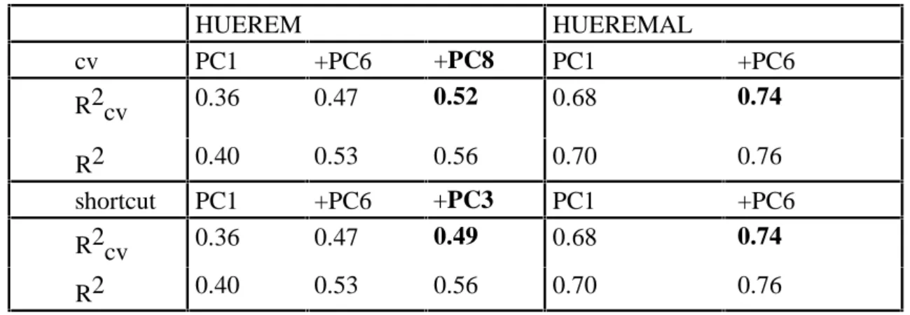
Example 3 (Production of a dyestuff, cp. Weihs and Jessenberger, 1999). In this example, based on 93 observations of 18 chemical analytical properties two measures of the hue of a dyestuff on fiber are to be predicted. The hue was measured under daylight (HUEREM) and under artificial light (HUEREMAL). Principal components analysis was applied to the correlation matrix. Stepwise variables selection based on predictive power then selects the 1^st (PC1) and the 6^thprincipal component (PC6) as the most influential on both the targets. Thus, for, e.g., (the mean centered) HUEREMAL the following models are selected:

HUEREMAL = β1 PC1 + ε and HUEREMAL = β1 PC1 + β2 PC6 + ε.

The same is also true for the proposed shortcut method. For HUEREMAL only these two principal components are selected. For more than two components R²cv decreases. For HUEREM, however, a third principal component increases predictive power, namely PC8 with greedy variables selection and PC3 with the shortcut. Naturally, PC3 gives a lower R²cv

than PC8, but has a bigger standardized regression coefficient. Table 3 shows predictive power and goodness of fit for the corresponding models for the two targets.

Table 3: Goodness of fit and predictive power

HUEREM HUEREMAL

cv PC1 +PC6 +PC8 PC1 +PC6

R2cv 0.36 0.47 0.52 0.68 0.74

R2 0.40 0.53 0.56 0.70 0.76

shortcut PC1 +PC6 +PC3 PC1 +PC6

R2cv 0.36 0.47 0.49 0.68 0.74

R2 0.40 0.53 0.56 0.70 0.76

5. Experimental Studies

In this section we will discuss two kinds of experimental studies, namely screening and optimization experiments, and contrast the application of variables selection in such studies to

5.1 Screening

In screening, linear models are used with coded influential factors.

Screening model

A screening model is of the form:

∑ ( )

= + +

+

= ^K

j

i i j c

i x iiN

y ij

1

2 1

1 β ε ,ε ~ .. 0,σ

β ,

where yi is the result of the target y in the i^th trial, xcij the coded level of the j^th factor in the i^thtrial, β1the increment, βj+1 the half effect of the j^thfactor on y,εi the error in the i^th trial and σ2 the error variance. In matrix form one can write:

ε β +

= X

y , where

















= A

X 1 1 M

is the design matrix including the plan matrix A with the column representation A = (xc1 ... xcK), where xcj = (xc1j ... xcnj)^T.

I.e. X is a matrix with all ones in the 1^st column and the columns of the matrix A.

β:= (β1β2...βK+1)^Tis the vector of the unknown model coefficients and ε:= (ε1 ... εn)^Tis the error vector.

The n rows of the plan matrix A correspond to the n trials, the K columns to the controlled factors. Each factor takes only two levels which are coded −1 and +1.

Such a plan matrix defines a screening plan iff the coded factors all have mean 0 and are pairwise orthogonal, _{i.e. xc}

j

Txck= 0, j≠k.

Note that in a screening plan A each column consists of exactly as many −1 as +1 in order to guarantee mean 0 for each factor, and that from these two properties it follows that X^TX = n⋅I.

Note that such screening plans are D-optimal (see, e.g. Cheng, 1980).

From the definition of screening designs it can be easily seen that all such designs fulfill the conditions a) and b) in section 3.2 so that they are very well suited for leave one out cross

validation. Moreover, the shortcut version of greedy variables selection based on the size of factor effects can be used as motivated in that section.

The structure of the design guarantees that the least squares estimates of the unknown coefficients have a simple form, that the effects can be determined independently, and that all estimated effects have the same estimated variance.

Computation of the least squares estimates

Since X′X = n.I, it is true that: ^{β$ =}

(

)

( )

ˆ) ˆ (

2

2 I

v o

C β = σ X′X ⁻¹ = σn

The aim of screening is factor reduction. Thus, again, the question is how to distinguish between relevant and irrelevant factors. This, naturally, is a task for a variables selection method. In screening experiments, conditions for stepwise regression with greedy forward selection turn out to be extremely favorable. Indeed, from the definition of screening designs it can be easily seen that all such designs, i.e. all fractional factorial designs and Plackett- Burman designs, fulfill both the conditions a) and b) in section 3.2 so that in screening the shortcut version of greedy variables selection based on the size of factor effects can be used as motivated in that section.

Therefore, on the one hand the screening situation is comparable to principal components regression as the different factors are uncorrelated and their effects can thus be determined independently, i.e. without considering the other factors. This means that a target cannot be adequately modeled without a factor with a big effect since the other factors cannot replace its effect. In contrast to principal components regression, however, in screening the designed factor levels additionally have a well known and simple form which leads to an observational balance in the sense of condition a) in section 3.2 and to the fact that the estimated regression coefficients are equal to half the effects of the involved factors on the target measured by the difference of the target means on the high level (= +1) and the low level (= -1) of the factor.

Altogether, in screening the size of the estimated regression coefficient itself is an indicator for the influence of the factor on the target, and in screening the shortcut variables selection method proposed in section 3.2 has the following form.

Greedy variables selection in screening experiments

In screening experiments, stepwise regression with greedy forward selection first selects the factor with the largest effect, then the factor with second largest effect, etc. until the predictive power is no more increasing.

In the following example it is demonstrated that this procedure might be a poor variable selector in the case of saturated orthogonal designs like Plackett-Burman designs as indicated at the end of section 3.2.

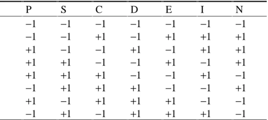
Example 4 (Wastewater purification plant, cp. Weihs and Jessenberger, 1999): The aim of this experiment is the reduction of the suspended solids in wastewater by means of a purification plant. The target thus is the reduction rate (%) which should be maximized. As possible influential factors were identified: ph value (P), salt amount (S), concentration (C), aeration intensity (I), entrance point (E), aeration duration (D) and plant no. (N). The design matrix X was chosen to have the form as in Table 4. Thus, X′X = 8.I!

For the screening plan in Table 4 the following reduction percentages were observed in the above ordering of the trials: 11, 29, 43, 8, 20, 4, 5, 16. The screening model for the target

‘reduction’ in the coded factors without elimination of irrelevant factors is of the form:

tion c

redu ˆ _{=17 + 2.Pc−5.Sc−2.5.Cc−0.Dc−}2.5.Ec + 10.Ic + 4.Nc.

Table 4: Plackett-Burman design

P S C D E I N

1 −1 −1 −1 −1 −1 −1 −1

1 −1 −1 +1 −1 +1 +1 +1

1 +1 −1 −1 +1 −1 +1 +1

1 +1 +1 −1 −1 +1 −1 +1

1 +1 +1 +1 −1 −1 +1 −1

1 −1 +1 +1 +1 −1 −1 +1

1 +1 −1 +1 +1 +1 −1 −1

1 −1 +1 −1 +1 +1 +1 −1

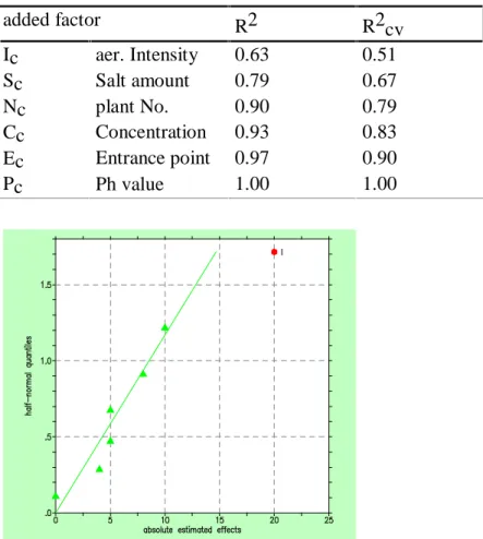
Table 5 shows the performance measures R2 and R2cv for the factors chosen by stepwise regression with greedy forward selection. In contrast, significance testing at the 5% level and the half normal plot (cp. figure 4) only identify the factor Ic with the biggest effect as significant.

Table 5: Goodness of fit and predictive power with stepwise regression

added factor R2 R2cv

Ic aer. Intensity 0.63 0.51

Sc Salt amount 0.79 0.67

Nc plant No. 0.90 0.79

Cc Concentration 0.93 0.83

Ec Entrance point 0.97 0.90

Pc Ph value 1.00 1.00

Figure 4: Half normal plot of effects on reduction (as generated by STAVEX, 1995)

5.2 Optimization

Near to an optimum, e.g. inside an ‘inverted cup’ region, the target cannot be represented adequately by a linear model in the influential factors alone, one needs a quadratic model in the factors, at least. As an optimization model we, thus, use a quadratic model in those factors which were selected to be relevant for the target in earlier stages of experimentation. Note that in what follows we restrict attention to quantitative influential factors.

Optimization model

In an optimization model, the target is modeled as a linear model in the coded factors, in their two-factor interactions, and in their squares:

( )

1

, 2 1

1

, 1

, 0 . .

~

,ε σ

ε β β

β

µ x x x x iiN

y _{i i}

K

j

j j cij K

j k j

k j cik cij K

j

j cij

i = +

∑

∑∑

∑

=

−

= >

=

,

where yi is the result of the target in the i^th trial, xcij the coded level of the j^th factor in the i^th trial, µ the intercept (overall mean), βj the coefficient of the j^th factor, βj,k the coefficient of the interaction of the j^th with the k^th factor, βk,k the coefficient of the squared k^th factor, εi the error in the i^th trial and σ2 the error variance.

A plan matrix defines an optimization plan iff all the involved coded factors take at least three different levels.

Note that for optimization models it is neither assumed that the coded factors only take values

−1 and +1 and have mean 0, nor that for the design matrix X it is true that X′X = n.I.

Therefore, the least squares estimates of the model coefficients are not interpretable as (half) effects of the factors, interactions or squared factors. The only condition a plan matrix has to fulfill is that all the involved factors take at least three different levels, because otherwise the effect of the squared factors is not estimable.

For the selection of optimization plans it is particularly important that the target is observed in sufficiently many points in the region of interest in order to be able to estimate the coefficients of the quadratic model reliably. Since the optimum will probably lie in a point of the region of interest in which no trial was carried out, the model has to be valid in the whole region. In order to avoid overfitting, we propose variables selection also for optimization models of the above kind. Since the aim of optimization modeling is a good prediction of the target in the optimum, at least, we propose to use predictive power, i.e. R2cv, as the selection criterion.

The results of section 3.2 indicate that for variables selection it is important to choose the experimental design in such a way that for each model to be compared the d_i are as equal as possible. Unfortunately, in optimization neither this condition a) nor the orthogonality of the factors in condition b) will be fulfilled in general. Thus the conditions for variables selection with cross validation are comparable to those of our starting example in section 4.1 where we were looking for an interpretation of principal components.

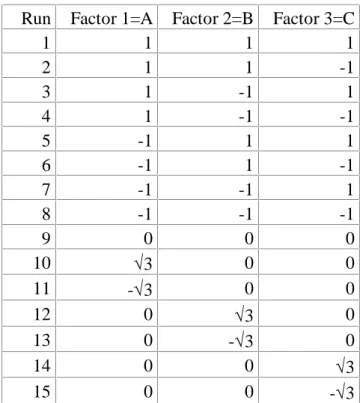
We begin with an example of a design with a particularly poor performance. Assume we have three factors, and we want to run an efficient design in 15 runs. Then we might want to use a

rotatable design, where the factors are set as in table 6. An interesting feature is that for this design d9 = 0 for all models that contain all three quadratic effects. Therefore, the model choice with the help of cross validation does not work properly for this design: No matter how big the effects of the squared factors may be, cross validation will never select a model with all three of them.

Table 6: A rotatable design in three factors and 15 runs Run Factor 1=A Factor 2=B Factor 3=C

1 1 1 1

2 1 1 -1

3 1 -1 1

4 1 -1 -1

5 -1 1 1

6 -1 1 -1

7 -1 -1 1

8 -1 -1 -1

9 0 0 0

10 √3 0 0

11 -√3 0 0

12 0 √3 0

13 0 -√3 0

14 0 0 √3

15 0 0 -√3

This would be different, if the run in the center point (run 9) is doubled, though. In the following example, another design with 15 runs is chosen. Here, the diare not so different and therefore the model search with RSS_cv works reasonably well.

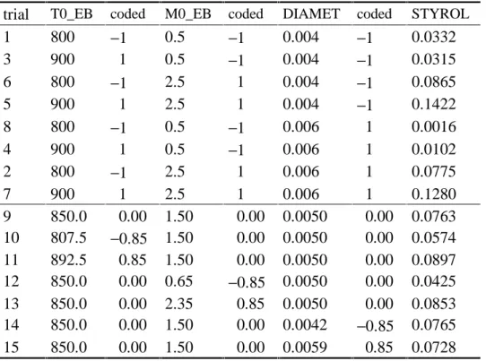
Example 5 (Optimization of the Styrol process, cp. Weihs and Jessenberger, 1999). In order to optimize the factor levels for the production of Styrol, an inscribed central composite design was used. This design was chosen in order to be able to use results from an earlier screening experiment so that the augmented design does not exceed the original experimental region. Table 7 shows the used design and the corresponding results of Styrol yield. The first eight trials were, in another ordering, already carried out in screening. The reported trial no.

corresponds to the screening ordering. The columns headed ‘coded’ show the coding of the column to their left.

The full quadratic model is of the form:

STYROL = β1 +β2⋅T0_EBc +β3⋅M0_EBc +β4⋅DIAMETc +β1,1⋅T0_EBc2 +β2,2⋅M0_EBc2 +β3,3⋅DIAMETc2 +β1,2⋅T0_EBc⋅M0_EBc +β1,3⋅T0_EBc⋅DIAMETc +β2,3⋅M0_EBc⋅DIAMETc +ε

Table 7: Inscribed central composite design

trial T0_EB coded M0_EB coded DIAMET coded STYROL

1 800 −1 0.5 −1 0.004 −1 0.0332

3 900 1 0.5 −1 0.004 −1 0.0315

6 800 −1 2.5 1 0.004 −1 0.0865

5 900 1 2.5 1 0.004 −1 0.1422

8 800 −1 0.5 −1 0.006 1 0.0016

4 900 1 0.5 −1 0.006 1 0.0102

2 800 −1 2.5 1 0.006 1 0.0775

7 900 1 2.5 1 0.006 1 0.1280

9 850.0 0.00 1.50 0.00 0.0050 0.00 0.0763 10 807.5 −0.85 1.50 0.00 0.0050 0.00 0.0574 11 892.5 0.85 1.50 0.00 0.0050 0.00 0.0897 12 850.0 0.00 0.65 −0.85 0.0050 0.00 0.0425 13 850.0 0.00 2.35 0.85 0.0050 0.00 0.0853 14 850.0 0.00 1.50 0.00 0.0042 −0.85 0.0765 15 850.0 0.00 1.50 0.00 0.0059 0.85 0.0728

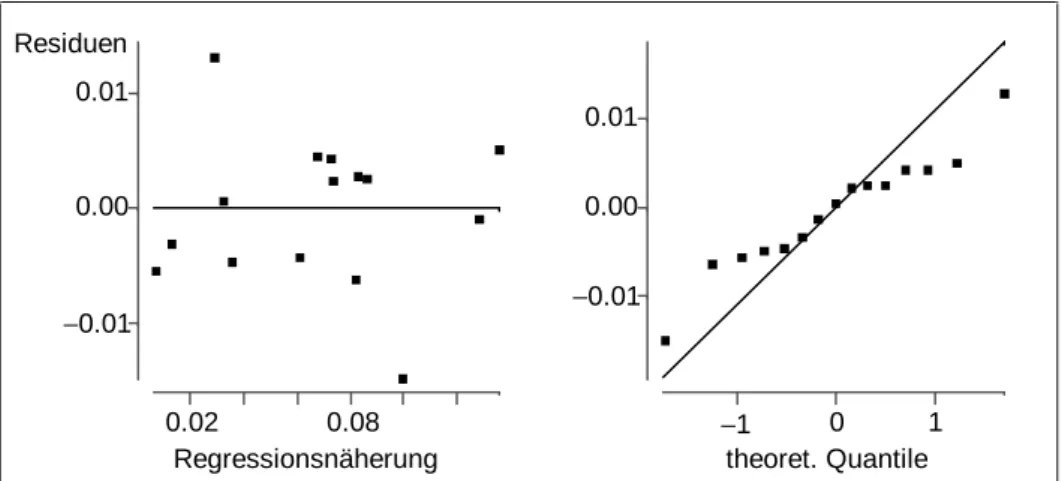
Model diagnostics of the estimated model shows a very acceptable goodness of fit, R2 = 0.98, and the residual plot in Figure 5 shows no structure. The normal plot in Figure 5, however, indicates a distribution of the residuals which is narrower than the normal distribution which results from estimating error expectation and variance by their empirical counterparts.

Table 8 shows the predictive power R2cv, and the corresponding measure for the goodness of fit R2 relevant for the selection of the first variable by means of variables selection.

Obviously, the best selection is the ‘Mass stream of EthylBenzol’ M0_EB.

Then, models with increment, M0_EB, and one more factor, two more factors, etc. were tried.

In the second step, i.e. after having added M0_EB, T0_EB increase the predictive power most so that this factor is added to the model. Etc. until in the 6^th step no increase of predictive power is possible. Thus, the resulting model includes five influential factors including one interaction and one squared factor:

STYROL = β1 + β2⋅T0_EBc +β3⋅M0_EBc +β4⋅DIAMETc +β1,2 ⋅T0_EBC⋅M0_EBc +β2,2 ⋅M0_EBc2 +ε .

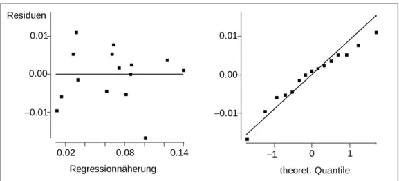
Model diagnostics of the estimated model leads to acceptable residual and normal plots (see Figure 6). Thus, variables selection may even lead to improved models.

−1 0 1

theoret. Quantile

−0.01 0.00 0.01

0.02 0.08

Regressionsnäherung

−0.01 0.00 0.01 Residuen

Figure 5: Residual plot and normal plot of the residuals in the full optimization model for STYROL

Table 8: Predictive power and goodness of fit of models for STYROL with increment and one (coded) factor only

Factor R2cv R2

T0_EB −0.3018 0.0971

M0_EB 0.6687 0.7640

DIAMET −0.3910 0.0310

T0_EB2 −0.2686 0.0058

M0_EB2 −0.2458 0.0170

DIAMET2 −0.2786 0.0049

T0_EB ⋅M0_EB −0.4121 0.0572

T0_EB ⋅DIAMET −0.4995 0.0001 M0_EB ⋅DIAMET −0.4918 0.0051

Table 9 tries to give an overview on the performance of cross validation for model choice if either the design from Example 5 is used, or if the rotatable design is used. The entries in Table 9 are the

∑

Hence, they indicate the expected size of RSS_cv if all the relevant factors are already in the model. For comparison we also give the lower bound n²/(n-K-1) which is achieved by an ideal design with all di equal. Note that if two models differ too much in

∑

∑

0.02 0.08 0.14 Regressionnäherung

−0.01 0.00 0.01 Residuen

−1 0 1

theoret. Quantile

−0.01 0.00 0.01

Figure 6: Residual plot and normal plot of the residuals after variables selection Table 9: Expected RSScv if there are all active effects included in the respective model Factors in the model Bound Design from Ex. 5 Rotatable design

A 17.30 17.36 17.42

A, B 18.75 18.97 18.90

A, B, C 20.45 21.07 20.54

A, B, C, AB 22.5 24.38 22.88

A, B, C, A² 22.5 23.07 23.57

A, B, C, AB, AC 25 29.95 26.47

A, B, C, A², B² 25 25.26 26.89

A, B, C, AB, AC, BC 28.125 41.31 32.67

A, B, C, A², B², C² 28.125 28.65 ∞

A, B, C, AB, AC, BC, A² 32.14 49.80 35.71

A, B, C, AB, AC, BC, A², B² 37.5 53.72 39.07

A, B, C, AB, AC, BC, A², B², C² 45 57.91 ∞

The table shows that for all models the design from Example 5 promises to provide a reasonable RSScv, while the rotatable design with 15 runs collapses for the models which contain all quadratic effects. Note that the design from Example 5 prefers models with fewer interactions if the number of factors is fixed.

6. Conclusion

In this paper we discussed the pros and cons of cross validation for variables selection using experimental design. On the one hand, we illustrated that experimental studies provide a