Callisto: Induction Signals

C allisto :

I nduction S ignals _, A tmosphere and P lasma I nteraction

I n a u g u r a l - D i s s e r t a t i o n zur

E rlangung des D oktorgrades

der M athematisch -N aturwissenschaftlichen F akult at ¨ der U niversit at zu ¨ K¨ oln

vorgelegt von

M ario S eufert

aus S chweinfurt

K¨ oln , 2012

Berichterstatter: Prof. Dr. Joachim Saur

(Gutachter) Prof. Dr. Fritz M. Neubauer

Tag der mündlichen Prüfung: 08.10.2012

To my beloved son David.

May the spirit of the Enlightenment guide you

through a long, pleasant and cheerful life.

Abstract

Callisto’s magnetic field environment and ionosphere are examined using a model for the magnetic fields induced in the satellite’s interior and 3D magnetohydrodynamic (MHD) simulations for Callisto’s interaction with the Jovian magnetospheric plasma. The in- duction model is also applied to the other Galilean moons Io, Europa and Ganymede to investigate the inductive responses of the satellites assuming the existence of interior conductive ocean and core layers.

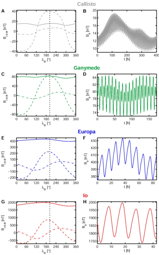
The first part of this thesis includes a thorough study of the frequencies and amplitudes of the temporary variable part of the magnetospheric field i.e., the inducing or primary fields and the strength of the induced or secondary fields originating in the interiors of the satellites. The primary fields are determined by using models for Jupiter’s intrinsic field, fields generated by the magnetospheric current sheet and fields caused by Chapman- Ferraro currents at the magnetopause boundary. A Fourier analysis of the magnetic field time series along the Galilean moons’ orbits predicted by this composite magnetospheric model yields the frequencies and amplitudes of the primary fields. A second model for the inductive response of a multi-layered conductivity structure based on two separate interior models for each satellite is applied to study the strength of the secondary fields at the surface. The synodic rotation period of Jupiter ( ∼ 10 h), the orbital periods of the satellites (from 42 h at Io to 400 h at Callisto) and the solar rotation period (642 h) are identified as the primary periodicities for the inducing fields at the Galilean moons. It is further shown that conductive ocean layers at Callisto and the other satellites should generate detectable magnetic signals for several frequencies in the vicinity of the satellites. The inferred strength of the signals at the surface ranges from 16 nT at Callisto to 210 nT for a magma ocean at Io. Possible conductive core layers, however, do not significantly modify the signals outside the satellites.

The interaction of the magnetospheric plasma with the atmosphere and interior of the

satellite has been extensively studied for the cases of Io, Europa and Ganymede. The

second part of this work represents the first in depth numerical study of Callisto’s plasma

interaction. A 3D MHD model, taking into account collision, ionization and recombina-

tion processes due to the neutral atmosphere of the satellite, is used to examine Callisto’s

ionosphere and magnetic field environment. In addition to the expected modifications of

the magnetospheric plasma flow embodied e.g., by the generation of Alfvén wings and

the upstream pileup of the magnetic field, the model results indicate a complex behavior

of the plasma flow in Callisto’s tail. The model predicts the existence of extended regions

where an oppositely directed plasma flow is associated with vertical eddy structures and

disturbances of the regions downstream of the Alfvén wings. The plasma densities within

the simulation are compared to measured electron density profiles to investigate the un-

derlying reason for the inferred dependence of the generation of an ionosphere on the

solar illumination of Callisto’s ram side. A parameter study performed for different con-

figurations of the neutral atmosphere shows that an atmosphere primarily confined to the

upstream hemisphere of Callisto suitably explains the measured variability of the iono-

spheric plasma densities. Additional reasons for this variability are varying conditions

for the magnetospheric plasma flow, differences in the solar photon flux and differences

in the plasma particle transport towards Callisto’s flanks depending on the solar illumina-

tion geometry. So far, observations of Callisto’s airglow yield no direct evidence for the

existence of an O

atmosphere. The interaction model predicts a disk integrated auroral

intensity of ∼ 6 R for earthbound measurements. This value is in agreement with the upper

limit of 15 R determined by Strobel et al. (2002). The simulation results for several flyby

scenarios are compared to magnetic field data taking into account the predicted induced

fields. Even though the plasma interaction signatures give rise to ambiguities regarding

the secondary field strength, the existence of a conductive interior ocean layer is inevitable

in order to explain the measured data. An ocean at a maximum depth of ∼ 150 km, with

a thickness of ∼ 10 km and a conductivity of sea water ( ∼ 5 S m

), which is in agreement

with an interior model by Kuskov and Kronrod (2005a), yields induced signals within the

plausible range suggested by the observations. The hypothesis of an asymmetric neutral

atmosphere is consistent with both radio occultation and magnetometer measurements

performed by the Galileo spacecraft.

Zusammenfassung

In der vorliegenden Dissertation wird die mögliche Existenz eines unterirdischen Wasser- ozeans, die Variabilität der Ionosphäre und der Aufbau der Neutralgasatmosphäre sowie die Plasmawechselwirkung des Jupitermondes Kallisto untersucht. Indizien für die Ex- istenz eines Ozeans bei Kallisto ergeben sich aus der Interpretation von Magnetfeld- daten der Raumsonde Galileo (siehe z.B. Khurana et al. 1998, Zimmer et al. 2000). Die gemessenen Magnetfeldstörungen werden Feldern zugeordnet, die aufgrund der zeitlichen Variabilität des magnetosphärischen Hintergrundfeldes in leitfähigen Schichten im In- neren des Mondes induziert werden. Die Existenz eines Wasserozeans mit einem aus- reichenden Anteil an gelösten Mineralien wäre eine plausible Erklärung für die Entste- hung induzierter Felder bei dem hauptsächlich aus Wassereis bestehenden Mond Kal- listo. Das Gesamtmagnetfeld in Kallistos Umgebung entsteht durch die Superposition verschiedener Teilfelder. Diese Felder umfassen das magnetosphärische Hintergrundfeld, mögliche induzierte Felder aus dem Inneren des Mondes und Magnetfelder, die bei der Wechselwirkung Kallistos und seiner Atmosphäre mit dem magnetosphärischen Plasma entstehen. Sowohl induzierte Magnetfelder als auch Magnetfeldstörungen die aufgrund der Wechselwirkung mit dem Hintergrundplasma entstehen, erzeugen zum Teil ähnliche dipolartige Signaturen. Eines der Hauptziele dieser Arbeit ist die Zuordnung der gemesse- nen Störungen zu möglichen Beiträgen zum Gesamtmagnetfeld und die Verifikation der Existenz induzierter Felder unter Berücksichtigung der Plasmawechselwirkung Kallis- tos. Mit Hilfe eines Modells, das sowohl eine Beschreibung des magnetosphärischen Feldes, als auch der im Inneren des Mondes induzierten Magnetfelder enthält, können die induzierenden oder primären Anteile des Hintergrundfeldes und der Beitrag der in- duzierten Felder zum gemessenen Signal vorhergesagt werden. Die Untersuchung der induzierten Feldanteile wurde mit Hilfe des für Kallisto entwickelten Modells auch auf die anderen Galileischen Monde ausgeweitet. Das für die Abschätzung der Magnetfeld- störungen die aufgrund der Plasmawechselwirkung entstehen benötigte magnetohydro- dynamische (MHD) Modell ermöglicht zudem eine Untersuchung der von Kliore et al.

(2002) gemessenen zeitlichen Variabilität der Ionosphäre Kallistos. Das entsprechende Modell gestattet die Analyse der möglichen Ursachen für die gemessenen niedrigen iono- sphärischen Plasmadichten im Fall einer sonnenbeschienenen, dem Plasmafluss entge- gengesetzt gerichteten Hemisphäre Kallistos. Neben diesen Hauptzielen der Arbeit wird zudem noch die allgemeine Natur der Plasmawechselwirkung bei Kallisto und die Inten- sität der Aurora Kallistos untersucht.

Das zur Erzeugung induzierter Felder notwendige, zeitlich variable induzierende oder

auch primäre Magnetfeld ist im Fall der Galileischen Monde durch das magnetosphärische

Feld Jupiters gegeben. In der vorliegenden Arbeit wird dieses Feld durch verschiedene Teilmodelle beschrieben. Es handelt sich um Modelle für Jupiters intrinsisches Mag- netfeld, für das Feld der magnetosphärischen Stromschicht und für die an der Magne- topausengrenzschicht durch Chapman Ferraro Ströme generierten Felder. Aus künstlich- en Zeitreihen für das magnetosphärische Feld entlang der Mondbahn werden die vorhan- denen Frequenzen und dazugehörigen Amplituden des primären Feldes bestimmt. Die Hauptfrequenzen des Primärfeldes sind durch die synodische Rotationsperiode Jupiters bezüglich der Monde ( ∼ 10 h), die Orbitalperiode der Monde (zwischen 42 h für Io und 400 h für Kallisto) und die Rotationsperiode der Sonne (642 h) gegeben. Als weitere Anregungsfrequenzen wurden ganzzahlige Vielfache der zuvor genannten Periodizität- en bestimmt. Mittels eines analytischen Modells für das induzierte oder auch sekundäre Feld eines sphärischen Körpers mit Schichten unterschiedlicher elektrischer Leitfähigkeit kann das an der Oberfläche der Monde messbare induzierte Feld bestimmt werden. Als Grundlage für die Leitfähigkeitsstruktur der Monde werden je zwei gängige Modelle des Mondinneren verwendet, die jeweils die mögliche Existenz eines Wasserozeans oder Magmaozeans (bei Io) berücksichtigen. Die induktive Antwort der Ozeane erzeugt für alle Monde deutlich messbare Magnetfelder bei verschiedenen Anregungsfrequenzen.

Der maximale Betrag der entsprechenden Felder liegt bei 16 nT für Kallisto und steigt auf bis zu 210 nT für Io. Die Bestimmung der Beiträge eines leitfähigen Kerns zum sekundären Feld an der Oberfläche zeigt, dass für keinen der Galileischen Monde eine deutliche Änderungen des Gesamtfeldes zu erwarten ist.

Im weiteren Verlauf der Arbeit werden die Wechselwirkung Kallistos mit dem magne- tosphärischen Plasma sowie die Ionosphäre und Neutralgasatmosphäre des Mondes un- tersucht. Während die Plasmawechselwirkung der anderen Galileischen Monde bereits Thema zahlreicher veröffentlichter Studien war, wird in dieser Arbeit das erste detail- lierte numerische Modell der Wechselwirkung Kallistos vorgestellt. Im Rahmen der MHD wurde ein Modell formuliert, das den Einfluss der Atmosphäre Kallistos auf das Hinter- grundplasma aufgrund von Stößen, Photo- und Stoßionisation sowie dissoziativer Rekom- bination beschreibt. Die allgemeine Struktur der Modellergebnisse für alle Plasmapa- rameter weist neben den erwarteten Signaturen der Plasmawechselwirkung, wie z.B. der Entstehung von Alfvénflügeln oder der magnetischen Pileup-Region in Anströmrichtung, zusätzliche komplexe Signaturen in der Schweifregion Kallistos auf. Innerhalb ausge- dehnter Bereiche stromabwärts des Mondes fließt das Plasma unerwartet in Richtung Kallistos. Die dazugehörigen Strömungen verursachen sowohl die Ausbildung vertikaler Wirbelstrukturen als auch signifikante Störungen der Alfvénflügel. Ein Vergleich der ionosphärischen Plasmadichten innerhalb des Simulationsgebietes mit den gemessenen Profilen der Elektronendichten von Kliore et al. (2002) erlaubt die Untersuchung der Ursachen für die Variabilität der Ionosphäre in Abhängigkeit der Richtung der solaren Einstrahlung. Eine Parameterstudie für verschiedene Geometrien und Zusammenset- zungen der Neutralgasatmosphäre ergibt, dass die gemessenen ionosphärischen Dicht- eschwankungen für verschiedene Positionen der Sonne relativ zur Richtung des anströ- menden Plasmas für eine asymmetrische, hauptsächlich auf die Anströmrichtung be- schränkte Atmosphäre, in Übereinstimmung mit den Messungen, deutlich erhöht sind.

Weitere Ursachen für die beobachteten Dichteschwankungen sind Änderungen der Pa-

rameter des Hintergrundplasmas, Variationen der Intensität der solaren Einstrahlung und

Zusammenfassung

der unterschiedlich stark ausgeprägte Transport ionosphärischer Teilchen an die Jupiter

zu- und abgewandten Flanken Kallistos für verschiedene Richtungen der solaren Ein-

strahlung. Eine Modellabschätzung der Intensität der bisher nicht eindeutig nachgewiese-

nen O

-Aurora Kallistos ergibt eine Gesamtstrahlung von 6 R für erdgebundene Beobach-

tungen. Dieses Ergebnis liegt innerhalb des bisher ermittelten oberen Grenzwertes für die

Strahlungsintensität von 15 R (Strobel et al. 2002). Der Vergleich der Modellergebnisse

für das Magnetfeld in Kallistos Umgebung mit den Galileo-Messungen für verschiedene

Vorbeiflüge zeigt, dass trotz ähnlicher Signaturen der induzierten und durch Plasmawech-

selwirkung erzeugten Magnetfelder eine Erklärung der Daten ohne die Berücksichtigung

induzierter Felder nicht möglich ist. Ein Wasserozean in 150 km Tiefe unter der Ober-

fläche, mit einer Ausdehnung von ungefähr 10 km und einer Leitfähigkeit nahe der irdis-

cher Ozeane von 5 S m

, erzeugt Induktionssignale, die innerhalb der vorgegebenen

Grenzen gut mit den Magnetfelddaten übereinstimmen. Ein solcher Ozean wäre zudem

konsistent mit gängigen Modellen für Kallistos Inneres (z.B. dem Modell von Kuskov

and Kronrod 2005a). Die Änderung der Signaturen der Plasmawechselwirkung aufgrund

einer asymmetrische Neutralgasverteilung ist ebenfalls konsistent mit den gemessenen

Werten für das Magnetfeld.

Contents

1 Introduction 1

1.1 The Jovian system . . . . 2

1.1.1 Properties of the Galilean moons . . . . 3

1.1.2 Jupiter’s magnetosphere . . . . 8

1.2 Induction signals and the plasma interaction of the Galilean moons . . . . 10

1.2.1 Induced fields: the ocean hypothesis . . . 10

1.2.2 Plasma interaction scenarios . . . 12

2 Induction signals of the Galilean moons 17 2.1 Observations and previous models . . . 17

2.2 Induction model . . . 18

2.2.1 Theory . . . 18

2.2.2 Model for the secondary fields . . . 21

2.2.3 Interior models . . . 22

2.2.4 Magnetosphere model . . . 25

2.2.4.1 Jupiter’s internal field . . . 25

2.2.4.2 Current sheet field . . . 26

2.2.4.3 Magnetopause field . . . 27

2.2.4.4 Variability of the magnetopause . . . 28

2.3 Results . . . 29

2.3.1 Primary fields . . . 29

2.3.1.1 The magnetospheric field at the Galilean moons . . . . 29

2.3.1.2 Spectral analysis . . . 30

2.3.2 Secondary fields . . . 36

2.3.2.1 Io . . . 36

2.3.2.2 Europa . . . 39

2.3.2.3 Ganymede . . . 41

2.3.2.4 Callisto . . . 44

2.3.2.5 Mutual induction . . . 46

2.3.2.6 Satellite measurements . . . 46

2.3.3 Conclusions . . . 48

3 Callisto’s plasma interaction 49 3.1 Observations and previous models . . . 49

3.1.1 Atmosphere and ionosphere . . . 51

3.1.2 Plasma environment . . . 52

3.1.3 Additional measurements . . . 54

3.2 Model description . . . 55

3.2.1 Theory . . . 55

3.2.2 Model equations . . . 58

3.2.2.1 Photo ionization . . . 60

3.2.2.2 Ionospheric particles . . . 62

3.2.2.3 Electron impact ionization . . . 63

3.2.2.4 Dissociative recombination . . . 66

3.2.2.5 Collisions . . . 67

3.2.3 Numerical implementation . . . 68

3.2.3.1 Boundary conditions and treatment of the interior . . . 69

3.2.4 Simulation setup . . . 70

3.2.5 Model scenarios . . . 71

3.3 Results . . . 75

3.3.1 The nature of Callisto’s plasma interaction . . . 75

3.3.1.1 Velocity and magnetic field . . . 75

3.3.1.2 Pressure, temperature and density . . . 79

Contents

3.3.1.3 Tail structures . . . 83

3.3.2 Neutral atmosphere and ionosphere . . . 89

3.3.2.1 Solar phase angle and atmospheric configurations . . . 89

3.3.2.2 Data comparison for the ionospheric densities . . . 94

3.3.2.3 UV aurora . . . 100

3.3.2.4 Currents and conductivities . . . 105

3.3.3 Comparison with magnetic field data . . . 108

3.3.3.1 C3 and C9 . . . 109

3.3.3.2 C10 and C22 . . . 115

3.3.4 Conclusions . . . 121

4 Summary 123 A Appendix 127 A.1 Maxwell’s equations . . . 127

A.2 Data comparison for C21, C23 and C30 . . . 128

Bibliography 133

1 Introduction

The four Galilean moons, named after their discoverer Galileo Galilei

, are among the most intensively studied planetary bodies. Io’s intensive volcanism, Europa’s shallow subsurface ocean and Ganymede’s intrinsic magnetic field are features that make these bodies unique compared to most of the other satellites in our solar system. The scientific attention received by the fourth of Jupiter’s lovers

Callisto to the present day is dwarfed by the long shadow of its sister satellites. Consequently, there are still numerous open questions regarding Callisto, some of which we try to enlighten in the course of this thesis.

One of the main tools scientists use today to study the satellites of our neighbor planets is the analysis of magnetic field data gathered by magnetometers on board various spacecraft visiting those bodies. Surface features such as the giant water plumes at Saturn’s satel- lite Enceladus, the interaction of the satellites and their atmospheres with their plasma environment and, by the analysis of intrinsic induced and dynamo magnetic fields, even their interior structure can all be studied using these data. Based on an analysis of the magnetic field perturbations measured by the Galileo spacecraft near the satellite it was concluded that Callisto, like Europa and possibly Ganymede, possesses an interior liquid water reservoir (Khurana et al. 1998, Neubauer 1998a, Kivelson et al. 1999, Zimmer et al.

2000). This presumably conductive ocean layer is exposed to the temporally variable Jo- vian magnetospheric field at Callisto’s position. Eddy currents generated inside the water layer give rise to induced magnetic fields detectable outside the satellite. However, the interaction of Callisto with the surrounding magnetospheric plasma also contributes to the magnetic field perturbations in the vicinity of the satellite. In some cases the plasma interaction can mimic induced field signals giving rise to some ambiguities in the inter- pretation of the data. The obstacle generating the magnetic field perturbations due to the interaction with the magnetospheric plasma consist not only of Callisto’s body it- self, but also of the intrinsic field due to the induction effect and both Callisto’s neutral atmosphere and ionosphere disturbing the plasma flow due to collisions, mass loading effects and the associated ionospheric conductivities. Therefore, a study for Callisto’s plasma interaction and induction signals also needs to include a suitable description of the processes occurring within the satellite’s atmosphere. In turn a comparison of the model results to magnetic field and other plasma data possibly yields information about Callisto’s atmosphere-ionosphere system.

I

* 02.15.1564 in Pisa; † 01.08.1642

II

according to Greek mythology

In the present work we deepen previous studies of the induced magnetic fields at Callisto and extend them by applying models for the plasma interaction of Callisto. An analysis of the possible induced fields is given in Chapter 2 of this thesis. Based on models for the magnetospheric background field and a model for the induced field generated within a layered sphere we infer the available amplitudes and frequencies of the inducing fields and predict the associated strength of the induced field at the satellite’s surface. The corre- sponding models developed to analyze Callisto’s induction signals were further applied to Io, Europa and Ganymede to obtain a complete picture of the possible induction signals at the Galilean moons. In Chapter 3 we present the first in depth study of Callisto’s plasma interaction. This study is based on a 3D magnetohydrodynamic (MHD) model of Cal- listo’s plasma environment using an extended version of the ZEUS-MP single-fluid MHD code (Hayes et al. 2006). Next to a general analysis of the plasma interaction processes at Callisto the model capabilities are used to infer information about Callisto’s atmosphere- ionosphere system. We analyze several possible reasons for the temporal variability of Callisto’s ionosphere observed by Kliore et al. (2002) and discuss possible configurations of the neutral atmosphere. Further we give predictions for the intensities of Callisto’s O

aurora whose existence was not conclusively verified to this date. Finally, we compare our model results to magnetic field data to analyze the plausibility of the assumption of an interior ocean layer generating induced fields, possible implications for Callisto’s neutral atmosphere and the general nature of the interaction signatures.

In this chapter we start with a short introduction to the Jovian system. Apart from the properties of Callisto relevant for the models and results presented in this thesis we dis- cuss properties of the other Galilean satellites for comparison and to establish the base for the induced field study in Chapter 2. Additionally, we shortly introduce the Jovian magnetospheric system which defines the ambient conditions for all Galilean satellites.

As induction and the plasma interaction effects are both relevant for the interpretation of the results obtained in Chapter 2 and Chapter 3, we also give a general introduction for these two processes in the present chapter.

1.1 The Jovian system

Jupiter and its satellites are often dubbed a miniature solar system embedded in our plan- etary system. Jupiter itself (Figure 1.1) is the largest of the outer planets’ gas giants with a mass of ∼ 1.9 × 10

kg and an equatorial radius (R

) of 71,492 km. Jupiter orbits the Sun with a perihelion of ∼ 4.95 AU

and an aphelion of ∼ 5.46 AU. The planet rotates about itself rather rapidly compared to most of the planets of our solar system, with a period of ∼ 10 h. So far 67 satellites of Jupiter have been discovered. The four Galilean moons Io, Europa, Ganymede and Callisto are, however, by far the most massive bodies in the Jovian system. The following section gives a short overview of the properties of these satellites.

III

1 AU ≈ 150 × 10

km. The distance between the Earth and the Sun.

1.1 The Jovian system

Figure 1.1: Jupiter view taken by the Cassini spacecraft (Courtesy of NASA / JPL / University of Arizona).

1.1.1 Properties of the Galilean moons Io, Europa and Ganymede

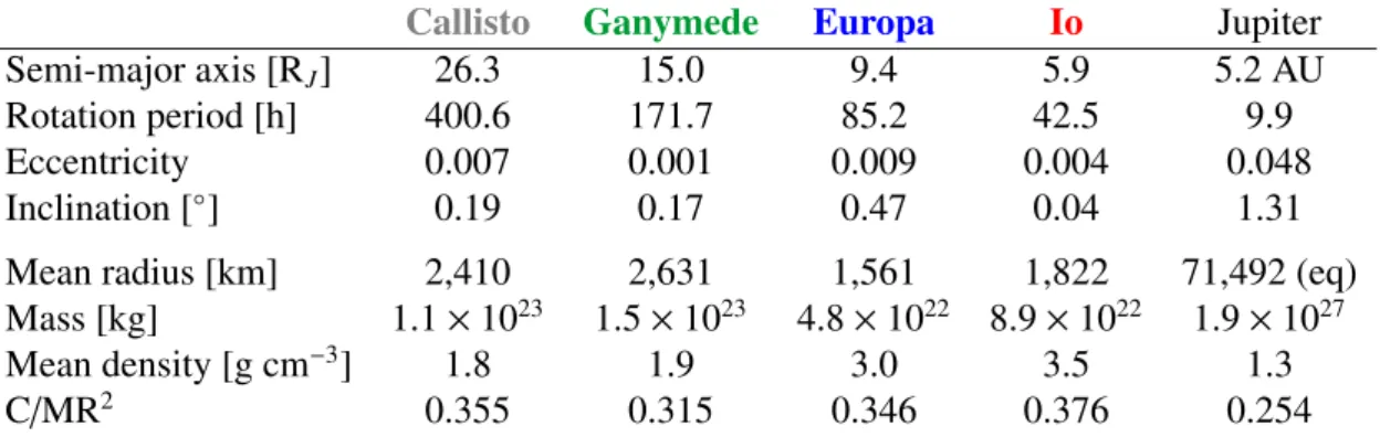
The four Galilean moons Io, Europa, Ganymede and Callisto (Figure 1.2) are compara- tively large, massive satellites for solar system standards (Table 1.1). Ganymede, in fact, is even the largest of all known satellites. While the two outermost satellites Callisto and Ganymede consist to a large extent ( ∼ 50 wt%

) of water ice (Kuskov and Kronrod 2005b), ice at Europa is primarily confined to a surface layer of ∼ 80 to 170 km thickness (Anderson et al. 1998). The innermost satellite Io is essentially depleted of water (McK- innon 2007). This general composition of the satellites is also reflected by their mean densities given in Table 1.1.

Figure 1.2: Global images of the Galilean moons (from left right: Io, Europa, Ganymede and Callisto) taken by the Galileo spacecraft (Courtesy of NASA / JPL / DLR).

IV

weight percent

Callisto Ganymede Europa Io Jupiter

Semi-major axis [R

] 26.3 15.0 9.4 5.9 5.2 AU

Rotation period [h] 400.6 171.7 85.2 42.5 9.9

Eccentricity 0.007 0.001 0.009 0.004 0.048

Inclination [

] 0.19 0.17 0.47 0.04 1.31

Mean radius [km] 2,410 2,631 1,561 1,822 71,492 (eq)

Mass [kg] 1.1 × 10

1.5 × 10

4.8 × 10

8.9 × 10

1.9 × 10

Mean density [g cm

] 1.8 1.9 3.0 3.5 1.3

C/MR

0.355 0.315 0.346 0.376 0.254

Table 1.1: Properties of the Galilean moons and Jupiter after Weiss (2004). For Jupiter the semi-major axis is given in AU and the radius refers to the equatorial value. The values for the normalized moments of inertia (C/MR

) were given by Anderson et al. (1996, 1998, 2001a,b) for the Galilean moons and Ward and Canup (2006) for Jupiter.

All of the Galilean moons perform synchronous rotations around Jupiter i.e., their or- bital and rotational periods are equal. The orbital paths of the satellites are not only defined by Jupiter’s strong gravitational field but are additionally influenced by strong 1:2:4 Laplace resonances between Io, Europa and Ganymede and a weaker 3:7 resonance between Ganymede and Callisto (Peale et al. 1979). These resonances, evident in the or- bital periods of the satellites, lead to enhanced eccentricities of the satellites’ orbits (Table 1.1). Due to these eccentricities all satellites perform a periodical movement inside Jupi- ter’s gravitational field which, in combination with the synchronous rotation, gives rise to strong tidal forces affecting their interiors and surfaces.

These forces are especially prominent at Io where they lead to an extensive tidal heating of the interior and to the most distinct surface volcanism in our solar system. According to several interior models of Io (e.g., Keszthelyi et al. 1999, Zhang 2003, Keszthelyi et al.

2004), tidal forces may hypothetically sustain a semi-liquid or mushy magma ocean layer.

However, such a global magma layer is not essentially necessary to create Io’s volcanism.

At Europa tidal heating is most likely the main energy source which maintains a subsur- face liquid water reservoir (Cassen et al. 1979). Additionally, tidal forcing may play a role in the generation of Europa’s surface features such as ridges and troughs (Greeley et al.

2004). Even though Ganymede’s surface shows to some extent similar surface structures, these features have an age of ∼ 2 Gyr, much older than at Europa (Pappalardo et al. 2004).

It is unknown if these structures were created by an ancient subsurface ocean layer. It is also not known whether such a layer is still present in the deep interior of Ganymede today.

The values for the normalized moments of inertia given in Table 1.1 indicate the internal

structure of the satellites. For a homogeneous sphere this value approaches C/MR

=

0.4. The low value of 0.315 for Ganymede points to a density concentration towards its

core. Models for Ganymede’s interior (e.g., Anderson et al. 1996, Zhang 2003, Kimura

et al. 2009, Bland et al. 2009) suggest a clear separation between an outer water ice

layer with a thickness of ∼ 1,000 km, a surrounding silicate mantle and a central iron

core whose extension is rather uncertain ( ∼ 500 to 1,000 km). Another evidence for a

distinct core layer at Ganymede is its intrinsic magnetic field discovered by the Galileo

1.1 The Jovian system spacecraft (Kivelson et al. 1996), which is likely generated in a central Fe or FeS layer (Schubert et al. 2004). Io, in contrast, shows almost no sign of a density concentration towards its center. One reason for this is the absence of water ice in Io’s composition.

Interior models (e.g., Anderson et al. 2001a, Zhang 2003, Keszthelyi et al. 2004) suggest a rough structuring in a thin lithospheric layer of ∼ 20 to 30 km, a partially molten mantle which probably shows a gradual increase in its density and a gradual decrease of the melt fraction and an inner core of ∼ 500 to 900 km thickness. Europa, finally, is primarily differentiated with an outer water ice shell up to a depth of 80 to 170 km, a chondritic mantle and a central Fe-FeS core with a radius of ∼ 450 to 650 km (e.g., Anderson et al.

1998, Kuskov and Kronrod 2005a). Besides gravity measurements used, for example, to infer the normalized moments of inertia, electromagnetic sounding using induced fields can provide valuable information about the Galilean moons’ interiors (e.g., Neubauer 1999, Saur et al. 2010). Determining the available signal amplitudes and frequencies for several interior models for all satellites is one of the key goals of the present thesis (Chapter 2).

All Galilean satellites possess tenuous atmospheres (McGrath et al. 2004). The primary atmospheric constituent at Io is SO

, with a mean column density of ∼ 10

to 5 × 10

cm

(Lellouch et al. 2007). The ultimate source of this atmosphere is Io’s volcanic activity, even though its generation may involve secondary processes such as sublimation of vol- canic material from the surface (Saur and Strobel 2004). In contrast, Europa’s O

atmo- sphere is generated by sputtering processes sustained by the bombardment of the satellites surface by energetic charged particles (Ip 1996, Saur et al. 1998). The molecular column densities of this atmosphere is considerably smaller than at Io and, according to Hall et al.

(1998), ranges between 2 × 10

to 14 × 10

cm

. The same authors report comparable values of 10

to 10

cm

for the column densities of an O

atmosphere at Ganymede.

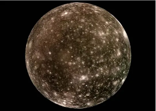
Callisto

Though Callisto (Figure 1.3) resembles Ganymede in its composition, size and location in the Jovian system, their interior structures show significant differences. Callisto’s con- siderably higher normalized moment of inertia (0.355 with respect to 0.315 at Ganymede, see Table 1.1) indicates that its interior is only partially differentiated (Anderson et al.

2001b). The reason for this dichotomy of the two largest Jovian satellites is still not com- pletely understood. One hypothesis by Barr and Canup (2010) states that Ganymede and Callisto took different paths in their thermal evolution, due to deviations in the energy input by impacts during the late heavy bombardment. Another possible hint may be the difference in the tidal heating (Showman and Malhotra 1997). While Ganymede is af- fected by Europa and Io due to their 1:2:4 resonance, Callisto only encounters a weak 3:7 resonance with Ganymede.

Whatever the reason for the dichotomy might be, it led to an interior structure of Callisto

which is best described by a continuous increase of the rock to ice composition ratio

towards the center of the satellite (Anderson et al. 2001b). Whether this increase occurs

continuously or stepwise is, however, not clear. Typical interior models for Callisto (e.g.,

Anderson et al. 2001b, Moore and Schubert 2003, Zhang 2003, Kuskov and Kronrod

2005a) involve three to six layers with an outer layer of nearly pure water ice which

may harbor a sublayer of liquid water, intermediate mantle layers with increasing silicate

Figure 1.3: Global images of Callisto taken by the Galileo spacecraft (Courtesy of NASA / JPL / Ted Stryk).

weight fractions and a core layer of pure silicate or iron-silicate mixtures. Valid core radii for Callisto range up to 1,300 km. The state of Callisto’s core is unclear. However, the absence of an internal dynamo field and the weak differentiation contradict the assumption of a pure iron core layer. The extension of the outer water ice shell is ∼ 300 km. It may contain a water ocean layer at a depth of ∼ 150 km with a maximum thickness of ∼ 180 km (Kuskov and Kronrod 2005a). In spite of the weak tidal heating at Callisto, this liquid layer could be preserved by internal radiogenic heat sources (Mueller and McKinnon 1988, Kuskov and Kronrod 2005a). The existence of an intrinsic liquid water ocean layer is also supported by magnetic field measurements (Neubauer 1998a, Khurana et al. 1998, Kivelson et al. 1999, Zimmer et al. 2000). The analysis of these magnetic signals using models of Callisto’s inductive response and, for the first time, its interaction with the magnetospheric plasma is the main motivation for this thesis. In the Chapters 2 and 3 we discuss to which extent Callisto’s interior layers contribute to the formation of the measured magnetic perturbations.

In contrast to the other Galilean moons, Callisto at first glance shows no evidence for ge-

ologic activity at its surface (Greeley et al. 2000, Moore et al. 2004). The most prominent

features on Callisto’s surface are crater structures (see Figure 1.3). Furthermore, Callisto

possesses the lowest albedo (0.2) of all Galilean satellites (Buratti 1991). This implies that

Callisto’s surface is comparatively old. There is, however, evidence for a crater degrada-

tion process on Callisto (Moore et al. 1999). Due to its low albedo, Callisto’s maximum

surface temperature is the highest of all Galilean moons and reaches values of ∼ 150 K

at noon (Hanel et al. 1979, Carlson 1999, Moore et al. 2004). Therefore, sublimation of

H

O occurs where the icy crust is exposed to free space. The remaining nonvolatile com-

ponents of the ice crust’s composition form a thin dark silicate layer. At steep slopes such

1.1 The Jovian system as crater rims the dust layer may be subject to mass movement, which in turn exposes new icy material. This procedure leads to a degradation of the crater rims and to a overall darkening of Callisto’s surface, in spite of the icy nature of the crustal layer below.

In analogy to Europa, sputtering of surface material plays a major role in the genera- tion of Callisto’s atmosphere (Kliore et al. 2002, Liang et al. 2005), even though the amount of magnetospheric energetic particles at Callisto’s orbit position is significantly lower (Moore et al. 2004). An additional source for the neutral atmosphere are H

O par- ticles sublimated on the surface. However, so far no successful direct measurements of the expected H

O and (due to dissociation processes) O

atmospheric components are available (Strobel et al. 2002). Instead, the Galileo Near-Infrared Mapping Spectrometer (NIMS) revealed the existence of a CO

atmosphere at Callisto with a surface density of

∼ 4 × 10

cm

(Carlson 1999) and a scale height of ∼ 23 km modeled for a surface pressure of 7.5 × 10

mbar. The source for this CO

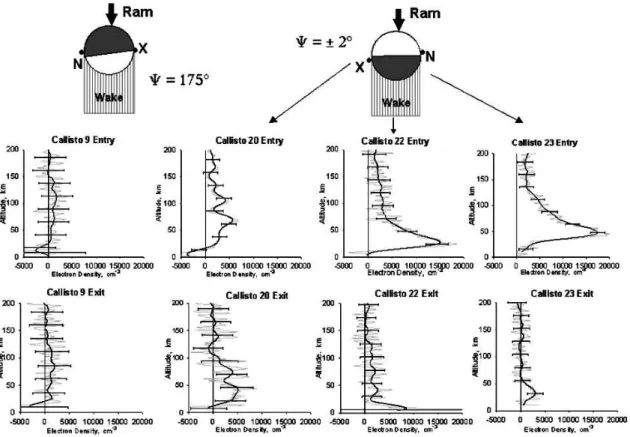
atmospheric component is not clear to this date. Another source of information for Callisto’s atmosphere are radio occultation mea- surements of the ionospheric electron densities (Kliore et al. 2002). The measured peak densities of ∼ 15,300 and 17,400 cm

during Galileo’s C22 and C23 flybys

are remark- ably high, compared to the ionospheres of the other Galilean satellites (e.g., 10,000 cm

at Europa according to Kliore et al. 1997). Such high values can not be explained by photo and impact ionization of the CO

atmospheric component alone. Kliore et al. (2002) pro- pose the existence of an undiscovered O

component with a surface density of ∼ 10

cm

to resolve this issue. The C9 radio occultation measurements of Galileo revealed no clear ionosphere signal beyond error bars. Kliore et al. (2002) suggest that the solar illumi- nation of Callisto’s ram side, encountered during the C22 and C23 flybys but not at C9, might be a necessary condition for the formation of an ionosphere. Liang et al. (2005) give a model for the neutral atmosphere which reproduces the above measurements taking into account an additional atmospheric O

component with a surface density of 7 × 10

cm

and a scale height of 30 km. Based on the chemistry in their model they also predict a significant H

O abundance with a surface density of ∼ 2 × 10

cm

and several minor species.

In the course of the present thesis, we simulate the C9, C22 and C23 plasma interaction scenarios to investigate the possible reasons for the differences in the ionospheric densities (Chapter 3). Further, models for a pure CO

atmosphere, models additionally considering an O

component and models assuming an asymmetric atmosphere generated by sput- tering are compared to the electron density and magnetic field data, to infer information about the state of the atmosphere. Both the induction model and the MHD interaction model presented in this thesis depend on the magnetospheric conditions at the location of Callisto and the other Galilean moons. The next section gives a brief introduction to Jupiter’s magnetospheric system to establish a base for the upcoming discussions.

V

For the numbering of the flybys “C” indicates a targeted encounter of Callisto and the appended

number denotes the orbit of Galileo around Jupiter.

1.1.2 Jupiter’s magnetosphere

While Jupiter as the largest planet in our solar system is still small compared to the Sun, its giant magnetosphere as an entity is the largest object of our solar system. The strength of Jupiter’s equatorial surface magnetic field is ∼ 420,000 nT, roughly 14 times stronger than at Earth (e.g., Acuna and Ness 1976, Connerney et al. 1998, Khurana et al. 2004).

The absolute strength of the field given by the magnetic moment is even 20,000 times larger than the terrestrial one (Kivelson and Russell 1995). The field rotates rapidly with the planet’s rotational period of 9 h 55 min. The magnetic axis is tilted ∼ 9.6

with respect to the rotational axis towards the right handed System III eastern longitude of ∼ 160

(200

western longitude, also see Figure 1.4). For definition of the System III coordinate system see e.g., the work of Dessler (2002) or Seidelmann and Divine (1977).

The magnetosphere is primarily populated by plasma produced by charge exchange ion- ization of neutral particles expelled by Io’s volcanoes (e.g., Bagenal and Sullivan 1981, Khurana et al. 2004). Roughly 1 t s

of plasma is inserted into the magnetospheric system by Io. Compared to other plasma supplies, such as the solar wind (100 kg s

) sputtering from the icy moons’ surfaces (20 kg s

) and the Jovian ionosphere (20 kg s

), Io is by far the most important plasma source (Khurana et al. 2004). Consequently, the plasma mainly consists of SO

as well as related ion species and electrons in a quasi neutral state (Krupp et al. 2004). The freshly produced plasma is electromagnetically

Figure 1.4: Sketch for the noon-midnight meridian of the Jovian magnetosphere after Khurana

et al. (2004). The angle between the vector denoted M which represents Jupiter’s magnetic axis

and the rotational axis given by Ω indicates the tilt of the magnetosphere. Black lines indicate the

field lines of the magnetospheric field. For the significance of the annotated regions not discussed

within this section the reader is referred to the original publication.

1.1 The Jovian system accelerated by Jupiter’s magnetic field. In the inner magnetosphere (up to ∼ 10 R

) the plasma velocities nearly reach the rotational speed of Jupiter. Initially, the plasma is mainly confined to a torus structure near Io, inclined by the tilt of the Jovian field with re- spect to the plane of the satellites’ orbits (see Figure 1.4). Interchange processes induced by centrifugal forces drive the plasma outwards in the horizontal direction. Additionally, electromagnetic mirror forces confine the plasma vertically to regions near the magnetic equator. These processes generate a plasma or current sheet layer with a vertical half thickness of ∼ 2 to 3 R

(Khurana 1997), stretching throughout the entire magnetosphere (For the generation of the plasma sheet see Khurana et al. 2004, Krupp et al. 2004, and references therein). The magnetospheric plasma flow generates its own, so called current sheet magnetic field which leads to a horizontal stretching of the originally quasi-dipolar field lines in the middle magnetosphere i.e., between 10 and 40 R

, as indicated in Figure 1.4 (also see e.g., Connerney et al. 1981, Behannon et al. 1981, Khurana and Kivelson 1993, Khurana 1997). In the region beyond ∼ 20 R

the plasma is significantly deceler- ated below corotational speed due to the inertial corotation lag (Hill 1979, 2001). The slow down of the plasma additionally generates a bending or sweep back of the field lines in the azimuthal direction (Khurana and Kivelson 1993).

Because of the tilt between the magnetic equator and the orbital plane and due to the rapid rotation of the Jovian magnetospheric field and the current sheet with respect to the satellite’s orbital period, Callisto is repeatedly exposed to different magnetospheric regimes. The satellite encounters conditions above and below the current sheet, where the surrounding magnetic field points primarily towards or away from Jupiter and the plasma density is relatively low. During current sheet crossings the plasma density at Callisto increases and the magnetic field points in the vertical direction. However, all of the actual flybys of Galileo at Callisto we consider in the course of this thesis took place away from the current sheets center.

The magnetosphere’s extension is confined by the magnetopause boundary depicted in Figure 1.4 (e.g., Engle 1992, Khurana et al. 2004). In this region the magnetic pressure of the Jovian magnetospheric field and the ram pressure of the solar wind cancel each other. Depending on the current solar wind conditions the location of the magnetopause subsolar point can vary approximately from 45 to 100 R

(Joy et al. 2002). The Galilean satellites are at all times located inside the Jovian magnetosphere. The downstream tail of the magnetosphere eventually extends beyond the orbit of Saturn at ∼ 9.5 AU (Khurana et al. 2004). Inside the magnetopause boundary layer a Chapman-Ferraro current system generates an additional contribution to the magnetic field (Chapman and Ferraro 1930).

This contribution generates a compression of the magnetic field lines on the solar wind ram side and an extension downstream.

The rotating Jovian magnetosphere is both the source for possible induction signals and

for magnetic perturbations due to the plasma interaction at the Galilean moons. In Section

1.2 we give an introduction to both of these effects relevant for the further discussions

within this thesis.

1.2 Induction signals and the plasma interaction of the Galilean moons

The magnetic field in the vicinity of Callisto and the other Galilean satellites shows sig- nificant perturbations with respect to the surrounding magnetospheric field. There are two main possible sources for those perturbations: First, magnetic fields generated in the interior of the satellite could contribute to the measured fields. These fields can origi- nate from dynamo generation processes inside the satellites’ core layers or from induced fields generated inside conductive interior layers. Secondly, the interaction between the impinging magnetospheric plasma and the satellite’s surface and atmosphere-ionosphere system generates exterior magnetic field structures which in some cases can mimic the essentially dipolar interior fields. We start this section with a discussion of the potential induced interior fields which led to the hypothesis of the existence of interior ocean layers inside all Galilean satellites.

1.2.1 Induced fields: the ocean hypothesis

The basic concept of the induction effect is that according to Maxwell’s equations (see Appendix A.1) a temporally variable magnetic field creates currents inside a electrically conductive body (e.g., Parkinson 1983, Schmucker 1985, Olsen 1999). For Callisto as well as for the other Galilean moons the variable magnetic field is provided by Jupiter’s magnetosphere (Neubauer 1999, Kivelson et al. 1999, Saur et al. 2010). The tilt of the magnetospheric field with respect to the satellites’ orbits and the fast rotation of the field structure leads to periodic variations of the background or primary field at the satellites’

locations. On the scale of the satellites’ sizes this variable field is primarily homogeneous.

The strength of the eddy shaped currents generated in a conductive interior of a satellite depends on the amplitude of the primary field and on the distribution of the conductivities.

The penetration or skin depth δ i.e., the depth at which the primary field generating the currents is reduced by a factor of e, defined by

δ =

s 2

σµ

ω , (1.1)

also depends on the conductivity σ and, additionally, on the frequency of the primary field oscillations ω. Equation (1.1) shows that low frequency inducing signals are able to penetrate deeper into the conductive interior. The induced currents themselves, in turn, generate induced or secondary magnetic fields. In the case of a spherical conductivity dis- tribution these fields have, to first order, a dipolar character (Parkinson 1983). This dipole is directed in opposite direction to the primary field and follows its temporal variations with a certain phase lag φ. The strength of the internal secondary field B

is commonly expressed in form of an relative amplitude A with respect to the external primary field B

i.e., A = B

/B

. For a perfectly conductive interior of a satellite A approaches unity, φ approaches zero and the secondary fields cancel the primary field at the surface.

At Callisto magnetic field perturbations which may be attributed to induced fields were

1.2 Induction signals and the plasma interaction of the Galilean moons measured during most of the flybys of Galileo at the satellite

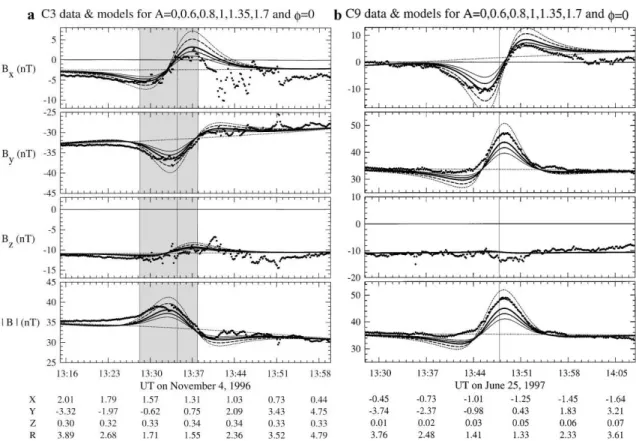
. Figure 1.5 shows the magnetic field data of the C3 and C9 flybys given in CphiO coordinates. For this Callisto- centric Cartesian coordinate system x points in the direction of rigid corotation, y points toward Jupiter and the z-axis is aligned with the Jovian rotational axis. Figure 1.5 ad- ditionally shows a data comparison by Zimmer et al. (2000) for several induced field models assuming different amplitudes A. The general structure of the measured magnetic field perturbations is fit remarkably well for models with A ≈ 1. Note that the given values of A = 1.35 and A = 1.75 correspond to models which account for a conductive ionosphere of Callisto. In analogy to the fields induced in the interior, a substantial iono- spheric layer can produce similar secondary fields which increase the measured relative amplitude. Further, based on the two flybys shown in Figure 1.5 an internal dynamo as a source for the perturbations can be ruled out. According to Zimmer et al. (2000), for the given C3 and C9 flyby geometries an intrinsic dynamo field would not generate fields pointing into different directions as visible in the B

component of Figure 1.5. An induced dipolar field, in contrast, does change its direction due to the different orientations of the primary field that Callisto encountered for both flybys. On the time scale of the Galileo mission (8 years in orbit) a pole reversal of an intrinsic dynamo field would be highly unlikely. Additionally, interior models of Callisto could hardly explain the existence of an internal dynamo for the proposed state of the core (e.g., Kuskov and Kronrod 2005a).

For the generation of the suggested induced fields a conductive layer needs to be present inside Callisto. The main constituents of the interior i.e., ices with an increasing contri- bution of silicates with depth, possess relatively low conductivity values, insufficient for the generation of induced fields with the observed strength. However, already a relatively thin water layer, liquefied by internal radiogenic heat sources as proposed for example by Kuskov and Kronrod (2005a), could generate substantial induced fields. Though the existence of other conductive sources such as iron rich layers cannot be completely ruled out, a water ocean layer is, from the geological standpoint, the most probable explanation for the observed perturbations. However, the results by Zimmer et al. (2000) allow no definitive conclusions about the depth, thickness and conductivity of the ocean.

Perturbation signatures similar to the ones mentioned above have been detected for all other Galilean moons. For Europa several induction and combined plasma interaction and induction models (e.g., Schilling et al. 2007, 2008) successfully proved the existence of an ocean layer in a depth of ∼ 10 km and with a thickness of ∼ 25 to 100 km for a proposed ocean conductivity above 0.5 S m

, close to the conductivity of terrestrial ocean water.

For Io a recent work by Khurana et al. (2011) claims the discovery of an interior magma ocean layer. For Ganymede so far no conclusive interpretation of the measured magnetic field perturbations was reached. The possible existence of an ocean at Ganymede might finally be resolved by the JUICE

mission which includes an orbiter around this satellite.

There is one caveat concerning the interpretation of the magnetic data at Callisto. So far the plasma interaction of this satellite was not adequately considered. Determining this contribution to the measured fields is one of the goals of this thesis. The next section gives an introduction to the concept of the plasma interaction at Callisto and its siblings.

VI

eight in total dubbed C3, C9, C10, C20, C21, C22, C23 and C30

VII

JUpiter ICy moons Explorer, see http://sci.esa.int/juice

Figure 1.5: Magnetic field data for the C3 and C9 Galileo flybys as well as model results for several relative amplitudes A of the induced field after Zimmer et al. (2000). Thick dots display the measured data. The modeled fields are shown for the cases: A = 0.6 (thinnest solid curve), A = 0.8 (solid curve of intermediate thickness), A = 1 (thickest solid curve), A = 1.35 (thick dashed curve), and A = 1.7 (thin dashed curve). The assumed phase lag for all models is φ = 0. The Jovian magnetospheric field is indicated by the thin dotted curve. The values below give the time labels, CphiO coordinates normalized to Callisto’s radius and the normalized distance to the satellites center. The shaded region indicates a crossing of the geometrical wake of Callisto

1.2.2 Plasma interaction scenarios

The nature of the interaction between the Jovian magnetospheric plasma flow and the satellites exposed to this flow has been extensively studied, especially in the case of Io (e.g., Piddington and Drake 1968, Goldreich and Lynden-Bell 1969, Goertz and Deift 1973, Neubauer 1980, Neubauer 1998b, Kivelson et al. 2004). A suitable theoretical framework to describe this interaction is the magnetohydrodynamic (MHD) approach (e.g., Kivelson and Russell 1995, Baumjohann and Treumann 1996). MHD theory treats the plasma as a fluid. Therefore, the movement of individual particles including, for ex- ample, the gyration of the plasma ions and electrons is neglected. This approach can be justified if the characteristic spatial and temporal scales of the flow are large compared to the scales of the kinetic processes. The macroscopic scales for the interaction are the satellite’s radius R and the plasma convection time τ

. These scales should be large com- pared to the gyro radii r

and periods τ

of the plasma ions to justify the fluid approach.

The respective values for the Galilean moons listed in Table 1.2 indicate that a MHD

description of Callisto’s interaction is justified only when the satellite is located outside

1.2 Induction signals and the plasma interaction of the Galilean moons the current sheet (see values for r

and τ

given in brackets), mainly due to the increased magnetospheric background field B

. All cases of Callisto’s interaction considered in the present thesis fall into this category. However, one needs to bear in mind that kinetic aspects of the plasma have more influence at Callisto than at the other satellites. Further, only stationary interaction scenarios are considered in the discussion below and for the models presented in this thesis. This is justified as the plasma convection time τ

is lower than the time scale of Callisto’s motion relative to the magnetospheric field, which lies in the order of tens of minutes to hours. It should, however, be noted that rapid fluctuations in the magnetospheric conditions frequently occur at Callisto. These small scale fluctuations are generally not predictable and therefore need to be neglected here.

All Galilean moons are exposed to a continuous flow of magnetospheric plasma which impinges on their trailing side due to the fast magnetospheric rotation with respect to the satellite’s orbital velocities. There are two main concepts for the description of the inter- action process within the MHD-framework (Saur et al. 2004): First, the interaction can be described by considering the perturbations of the plasma flow and the magnetic field (B, v picture), which generate a current system in the vicinity of the satellite. Secondly, currents and the associated electric fields generated by the interaction may alternatively be considered as the source of the magnetic disturbances (E, j picture). Essentially, both approaches are suitable to describe the nature of the interaction.

The drivers of the interaction are the deceleration of the plasma flow equivalently by electron and ion neutral collisions and by mass loading due to ionization processes within the satellite’s atmosphere (Neubauer 1998b). In the ideal MHD approach, valid outside of the satellite’s conductive ionospheric region, the magnetic field is frozen in to the plasma (e.g., Kivelson and Russell 1995, Baumjohann and Treumann 1996, also note Equation 1.4 below). Therefore, in the B, v picture the deceleration of the flow leads to an upstream

Callisto Ganymede Europa Io

B

, Jovian magnetic field [nT] 4 (42) 64 (113) 370 (460) 1720 (2080) v

, relative velocity [km s

] 192 (122-272) 139 (84-152) 76 (56-86) 57 (53-57) n

, ion number density [cm

] 0.10 (0.01-0.5) 4 (1-8) 130 (12-170) 1920 (960-2900) m

, average ion mass [amu] 16 (2) 14 (2) 18.5 (17) 22 (19) p, total pressure [nPa] 0.38 (0.39) 3.8 (3.9) 17 (26) 34 (54)

R, mean radius [km] 2410 2631 1561 1822

r

, ion gyro radius [km] 530 (34) 36 (13) 8 (12) 1.8 (1.6)

τ

, plasma convection time [s] 415 936 552 5460

τ

, ion gyro period [s] 262 (3) 14 (1) 3 (2) 0.8 (0.6)

M

, Alfvén Mach number 2.8 (0.02-8.5) 0.73 (0.05-1.1) 0.47 (0.08-0.59) 0.31 (0.16-0.39) M

, sonic Mach number 0.4 (0.03-1.2) 0.5 (0.06-0.8) 0.9 (0.16-1.1) 2.0 (1.0-2.1)

β, plasma beta 64 (0.6) 2.4 (0.8) 0.32 0.04

Table 1.2: Properties of the plasma flow at Callisto and the other Galilean moons after Kivelson et al. (2004). The given values refer to conditions at the magnetic equatorial plane i.e., inside the current sheet. Values in brackets correspond to conditions in the lobe regions outside the current sheet, or to minimum and maximum values for v

, n

, M

and M

. The values for τ

were adapted from Neubauer (1998b). The gyro periods were calculated using: τ

=

0q

, where q is equal to

the elementary charge.

pile up of the magnetic field lines and to an enhanced magnetic field magnitude. Away from the atmosphere the same magnetic field lines continue to move with their original velocity. This leads to a draping of the field lines around the satellite as depicted in the side view in Figure 1.6. Perpendicular to the magnetic field lines and the direction of the incident plasma the flow is diverted around the obstacle. The plasma velocity increases above the background value v

at these flanks. Behind the satellite the plasma flow is accelerated to its original speed due to the relaxation of the magnetic field lines caused by the magnetic tension. In this region the magnitude of the magnetic field decreases.

The flow pattern along the magnetic field lines is dominated by standing shear Alfvén waves which primarily propagate along this direction (e.g., Kivelson and Russell 1995, Baumjohann and Treumann 1996). These transverse waves are characterized by consecu- tive disturbances in the magnetic field and the velocity. Alfvén waves are able to transport energy and momentum along the magnetic field lines. Their wave speed is determined by the magnetic field B

and the mass density ρ of the plasma:

v

= B

√ µ

ρ . (1.2)

The actual direction of the Alfvén wave propagation is defined by the sum of the Alfvén velocity parallel and anti-parallel to the undisturbed magnetic field B

and the incident plasma velocity v

(Neubauer 1980):

C

: v

= v

± v

. (1.3)

The cylindrical regions starting from the cross section of the satellite (including its atmo- sphere) along the two Alfvén characteristics C

are called Alfvén wings. Their direction is indicated by thin solid lines in Figure 1.6. Inside the wings the plasma flow is signifi- cantly slowed down and the magnetic field is bend towards the direction of C

, while its magnitude remains unchanged.

In the view of the E, j picture, the electric field

E

= − v

× B

(1.4)

Figure 1.6: Sketch of Io’s plasma interaction for a side view and a view along the flow direction

after Saur (2004). The magnetic field structure is indicated by solid lines with arrows. The current

system is shown by dashed lines. The Alfvén wings are depicted by thin solid lines.

1.2 Induction signals and the plasma interaction of the Galilean moons of the plasma flow in the rest frame of the satellite, drives a current perpendicular to B

inside the conductive ionosphere of the satellite (see dashed lines in the front view of Figure 1.6). This current leads to a charge separation towards the two hemispheres of its direction and to an electric field whose Lorentz forces slow down the plasma flow and per- turb the magnetic field. Away from the satellite the conductivities perpendicular to B

are low but the conductivity along the field lines is high everywhere. Therefore, the current is continued along the magnetic field lines or, more precisely, the Alfvén characteristics.

The field lines guide the currents towards Jupiter’s ionosphere where the current system is closed. The carrier for the currents are, in fact, the Alfvén waves described above for the B, v picture. Apart from shear Alfvén waves, compressional slow and fast mode mag- netohydrodynamic waves are generated by the plasma interaction. Slow mode waves can also generate wing structures along their characteristics (Neubauer 1998b). However, the perturbations associated with those waves are generally much weaker.

The interaction process described above is only valid for subalfvénic flow velocities i.e., in terms of the Alfvén Mach number, for M

= v

/v

< 1. Superalfvénic flows gener- ate shock boundaries upstream of the obstacle, preventing the generation of Alfvén wing structures. While the flow at Io, Europa and Ganymede is primarily subalfvénic, Callisto repeatedly encounters superalfvénic conditions while moving through the center of the current sheet (see Table 1.2). Outside the current sheet the plasma conditions at Callisto also show distinct deviations compared to the other interaction scenarios. The magnitude of the magnetic field B

, the density ρ and the plasma pressure p are significantly lower in these regions. On the other hand, the flow velocities v

are considerably higher. Addition- ally, the plasma parameters at Callisto are highly variable. Therefore, various interaction scenarios with different interaction strengths and geometries are possible for this satellite.

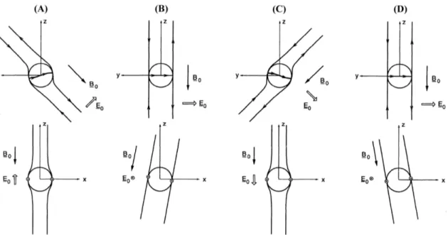
Fields induced in Callisto’s interior change the overall pattern of the interaction. Figure 1.7 shows the deviation of the Alfvén wing structures caused by a dipolar induction field discussed by Neubauer (1999). The wing cross sections are reduced and the wings are shifted with respect to the satellite (Figure 1.7A and 1.7C). The shape of the cross section in these cases is approximately cylindrical. Also, the maximum current which can flow through the wings is reduced. During current sheet crossings (Figure 1.7B and 1.7D) the induced field vanishes as the time variable primary fields approach their zero-crossings and the wings remain unaffected. This is, however, only the case if the flow retains its subalfvénic nature. As the magnetic signatures of Callisto’s plasma interaction depend on the orientation of the Jovian background field they are themselves temporally variable.

Therefore, they contribute to the induction effect which in turn modifies the interaction

field patterns. An entirely self-consistent formulation for a model analyzing the magnetic

perturbations needs to include this feedback processes (Neubauer 1999). The only inter-

action model accounting for this feedback was given for Europa by Schilling et al. (2007,

2008). Though the Callisto MHD model introduced in Chapter 3 closely follows the for-

mulation of these authors, the above feedback mechanism is not taken into account for

the results presented in this thesis. Still, the presented model gives the first numerical 3D

MHD description for Callisto plasma and magnetic field environment. Possible induced

signals are considered by using a separate model for the primary and secondary fields at

the Galilean satellites, introduced in the following chapter.

Figure 1.7: Callisto’s Alfvén wing pattern considering internal induced fields after Neubauer

(1999). The x-coordinate indicates the direction of the plasma flow. y is directed towards Jupiter

and z points in the direction of the Jovian rotational axis. (A) displays conditions at northern

magnetic latitudes and (C) the corresponding case below the magnetic equator (below the current

sheet). (B) and (D) display the geometry during current sheet crossings, if the condition M

< 1

is still fulfilled. B

and E

indicate the direction of the undisturbed magnetic and electric fields.

2 Induction signals of the Galilean moons

In this chapter we analyze the possible inductive response of the interior of Callisto. Addi- tionally, the established procedure is applied to Ganymede, Europa and Io. In a first step, we present a model for the secondary, induced fields generated for a spherical conduc- tivity distribution consisting of an arbitrary number of interior shells. Secondly, several interior models for all Galilean satellites are outlined. They define the conductivity struc- ture required as an input for the secondary field model. In a third step, models for the magnetospheric field of Jupiter i.e., the primary or inducing field are specified. Based on these models we infer various amplitudes and frequencies of the Jovian field at the orbits of the satellites. The obtained primary field amplitudes and frequencies are used to predict the associated amplitudes and phase shifts of the induced fields at all Galilean moons, based on the secondary field model. The procedures and results outlined in this chapter were in parts published by Seufert et al. (2011).

2.1 Observations and previous models

Distinct magnetic perturbations were measured in the vicinity of all Galilean satellites.

These measurements were recorded by the magnetometer on board the Galileo spacecraft (Kivelson et al. 1992) and can be obtained from the Planetary Data System

provided by NASA. At Callisto and Europa magnetic field anomalies were to some extent attributed to induced fields (Neubauer 1998a, Khurana et al. 1998, Kivelson et al. 1999). In analogy to similar models at Earth (e.g., Lahiri and Price 1939, Parkinson 1983, Olsen 1999, Con- stable and Constable 2004), several authors modeled the characteristics of those fields for Callisto (Zimmer et al. 2000) and Europa (Kuramoto et al. 1998, Zimmer et al. 2000, Schilling et al. 2008). Recently, Khurana et al. (2011) modeled the magnetic field envi- ronment at Io taking into account induction effects by a potential internal magma ocean.

Ganymede possibly also shows signatures of induced magnetic fields. However, Gany- mede’s internal dynamo field gives rise to some ambiguities regarding the interpretation of the observed magnetic field as outlined by Kivelson et al. (2002). In addition, several summaries of induced magnetic field studies are available in the literature (e.g., Jia et al.

2009, Saur et al. 2010).

I

http://pds.nasa.gov

Most of the above induction models consider simple one or two layer structures of the satellites’ interiors. Therefore, they potentially neglect geologic restraints which can be taken into account by assuming more complex multi-layer interior models. Additionally, most authors focus on the main primary field amplitudes and frequencies, such as the variations due to Jupiter’s internal dipole or the current sheet field in the case of Callisto.

Low frequency contributions from the primary signals, which potentially allow a deep sounding of the interior, are neglected in most of the previous surveys. We present the first thorough study of all available primary signal contributions at the Galilean moons, taking into account realistic multi-layer interior models. While the focus of the present thesis lies on Callisto, the models below are also applied to the other Galilean satellites. Section 2.2 introduces the model used to determine the induced field signals at all satellites.

2.2 Induction model

2.2.1 Theory

According to Maxwell’s equations (see Appendix A.1), temporally variable magnetic fields induce electric fields and therefore currents inside an electric conductor. Those currents in turn generate magnetic fields which act against the fields outside the conduc- tor. By combining Ohm’s, Faraday’s, Ampère’s law and Gauss’s law for magnetism, the following diffusion equation can be derived:

∂B

∂t = −∇ × 1

σµ ( ∇ × B)

!

. (2.1)

It describes the spatial and temporal evolution of the magnetic field B inside a medium with an electric conductivity of σ. The displacement currents in Ampère’s law are ne- glected here as the conduction currents are considerably larger for the relevant materials and appropriate time scales for the induction process at the Galilean moons (Saur et al.

2010). Further, for the diamagnetic and paramagnetic materials expected in the interiors of the satellites which possess a magnetic susceptibility of χ

≈ 0, µ can be assumed to be the vacuum permeability µ

. Also note that possible tidal motions inside the liquid or semi-liquid layers of the Galilean moons are neglected here. If we consider regions with a spatially constant conductivity, Equation (2.1) simplifies to:

∂B

∂t = 1

σµ

∆B. (2.2)

We now follow the approach of Parkinson (1983) to find solutions for Equation (2.2) for a spherical distribution of σ within an arbitrary number (s = 1 to S ) of shells. The conductivity inside the shells σ

is assumed to be constant, so that Equation (2.2) is valid for each layer. The background field B

which drives the induction, can be decomposed into its stationary contributions B

and time-variable contributions B

for N different frequencies ω

. It can be expressed by a Fourier decomposition of the form:

B

= B

+ B

= B

+ X

n=1

B

e

. (2.3)