phylogeography and seed banking
Dissertation zur Erlangung des Doktorgrades der Naturwissenschaften (Dr. rer. nat.) der Fakultät für Biologie und Vorklinische Medizin
der Universität Regensburg
vorgelegt von
MARTIN LEIPOLD
aus Schwandorf
im Jahr 2018
Regensburg, den 26.10.2018
Martin Leipold
Chapter 1
Chapter 2
Chapter 3
Chapter 4
Chapter 5
Chapter 6
Zusammenfassung References
Danksagung
6 8
20
26
40
48 50 52 61 General introduction
Sampling for conservation genetics: how many loci and individuals are needed to determine the genetic diversity of plant populations using AFLP?
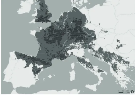
Species distribution model reveals suitable climates for oceanic species during the Last Glacial Maximum
Insights into the European postglacial colonization of the horseshoe vetch (Hippocrepis comosa)
Short communications of a seed bank for threatened plant species on the example of the Genbank Bayern Arche
Conclusions and perspectives
DECLARATION OF MANUSCRIPTS
Chapter 2 was published with the thesis’ author as main author:
Leipold, M., Tausch, S., Hirtreiter, M., Poschlod, P., & Reisch, C. (2018). Sampling for conservation genetics:
how many loci and individuals are needed to determine the genetic diversity of plant populations using AFLP? Conservation Genetics Resources: 1-10.
Chapter 3 and 4 were published with the thesis’ author as main author:
Leipold, M., Tausch, S., Poschlod, P., & Reisch, C. (2017). Species distribution modeling and molecular mark- ers suggest longitudinal range shifts and cryptic northern refugia of the typical calcareous grassland species Hippocrepis comosa (horseshoe vetch). Ecology and Evolution, 7(6), 1919-1935.
Chapter 5 was published with the thesis’ author as co-author:
Leipold, M., Tausch, S., Reisch, C., & Poschlod, P. (2019). Genbank für Wildpflanzen-Saatgut - Bayern Arche
zum Erhalt der floristischen Artenvielfalt. UmweltSpezial, Bayerisches Landesamt für Umwelt, Augs-
burg, 66 S.
VEGETATION, SPECIES RANGES AND SPECIES DIVERSITY
Global vegetation, habitat as well as species abun- dances and distributions have consistently changed during the course of Earth’s history (Schroeder, 1998).
Today’s natural plant distribution in Central Europe is the result of range shifts after the last glaciation and synchronous human impact (Lang, 1994; Taberlet et al., 1998; Poschlod, 2017). However, since the begin- ning of the modern age the rate and extent of envi- ronmental deterioration continuously increased due to human activities (Poschlod & WallisDeVries, 2002;
Poschlod, 2017).
The distribution of plant species would -with- out human interaction- mostly depend on climate, weather, soil and interspecific competition (Wood- ward, 1987). Despite other factors such as con- strained dispersal (Normand et al 2011), climate is the most influential natural broad-scale parameter for species’ ranges (Willis & Whittaker, 2002; Pearson
& Dawson, 2003). Without a suitable climate, a plant can’t germinate, repopulate, grow or reproduce in a habitat. Hence, for the prediction of future or the reconstruction of past plant species’ ranges, climate data can be used in species distribution models (SDM) (Elith & Leathwick, 2009). While such models point out the potential distribution of habitats of spe- cies, the analysis of genetic diversity and relatedness in phylogeographic studies can help to identify colo- nisation routes or glacial refugia (Taberlet et al., 1998;
Hewitt, 1999, 2004).
The human impact on ecosystems, vegetation composition and species distribution is significant:
climate change by rising atmospheric concentrations of carbon dioxide and other greenhouse gases, an- thropogenic nitrogen deposition, changing land use and altered disturbance regimes, deforestation and habitat destruction (Vitousek et al., 1997; Scheffer et al., 2001; Tilman et al., 2001).
Recent industrialisation accompanied with growth of human population have caused unprecedented se- vere loss of the three levels of plant biological diver- sity: habitats and ecosystems, species and communi- ties as well as plant genetic diversity. The European Red List of Habitats (Janssen et al., 2016) considers
36 % of the 233 habitats assessed (31 % for EU28+) as threatened: < 2 % as critically endangered, 11 % as endangered and 24 % as vulnerable. On the species level the red list of endangered plant species in Ger- many (Ludwig & Schnittler, 1996) states that 40 % of all native plants are at least very rare. On population level a number of factors like fragmentation and size of populations, genetic drift and bottlenecks strong- ly influence the genetic diversity and must therefore be considered when depicting the diversity of plants and the value and threats of single populations (Re- isch & Poschlod, 2003; Reisch et al., 2003; Reisch et al., 2005; Reisch & Kellermeier, 2007).
ACTIONS FOR PRESERVATION OF DIVERSITY
As a counterpart to previously ratified conservation strategies concerning animals and its habitats, the Global Strategy of Plant Conservation (GSPC) from 2002 for the first time focused on the prevention of further losses of plant biological diversity (CBD, 2010).
The GSPC contained 16 targets, which should stop or at least slow down the loss of phytodiversity by the year 2010. In 2010, when the failure was inevitable, the targets were updated at COP10 (Nagoya) and are expected to be implemented until 2020. The first two objectives (“Plant diversity is well understood, documented and recognized” and “Plant diversity is urgently and effectively conserved”) encompass
“Information, research and associated outputs, and methods necessary to implement the Strategy devel- oped and shared” (target 3) and “At least 75 per cent of threatened plant species in ex situ collections, pref- erably in the country of origin, and at least 20 per cent available for recovery and restoration programmes”
(target 8).
THESIS OUTLINE
The thesis at hand was prepared within the frame- work of the foundation of the Genbank Bayern Arche, a Bavarian seed bank for rare and threatened plant
CHAPTER 1
General introduction
QUESTIONS AND AIMS
The key elements that are addressed in this thesis are:
1. Sampling for conservation genetics: how many loci and individuals are needed to determine the genetic diversity of plant populations using
AFLP markers? (Chapter 2)
2. Species distribution model reveals suitable cli- mates for oceanic species during the Last Gla-
cial Maximum. (Chapter 3)
3. Insights into the European postglacial coloni- zation of the horseshoe vetch (Hippocrepis co-
mosa). (Chapter 4)
4. Short communications of a seed bank for threatened plant species on the example of the Genbank Bayern Arche. (Chapter 5) species. Its single chapters are supposed to help to-
wards achieving the targets of the GSPC.
In order to provide assistance for the collection of plant material for genetic studies based on AFLP markers (objective I) or for seed collections for ex situ conservation (objective II), Chapter 2 intends to iden- tify patterns in the assessment of genetic diversity of 16 different plant species of the habitat calcare- ous grasslands. The number of plant individuals that must be collected to reflect the genetic diversity of a single population can be important to increase effi- ciency and productivity through reduced sample siz- es. The study also investigates whether and to what extent plant functional traits have an influence on the sample size.
Using climate modelling in Chapter 3 as well as phylogeographic analysis in Chapter 4, this thesis provides further knowledge about the origin of cal- careous grasslands and thereby a better understand- ing of plant diversity (objective I). Numerous studies have examined calcareous grasslands from different perspectives (Cornish, 1954; Gibson & Brown, 1991;
Dutoit & Alard, 1995; Poschlod & Bonn, 1998; Po- schlod et al., 1998; Poschlod & WallisDeVries, 2002;
Kahmen & Poschlod, 2004; Karlik & Poschlod, 2009;
Römermann et al., 2009). But still, the origin of its plant inventory and the potential migration routes after the last glaciation are widely unknown. It is generally assumed that plants from Central Europe outlasted the ice age in Mediterranean refugia. Re- cent research also point to additional refugia north of the Alps (Provan & Bennett, 2008; Svenning et al., 2008; Tzedakis et al., 2013). We therefore conducted an AFLP analysis of the horseshoe vetch (Hippocrepis comosa) across the whole species distribution range to provide insights into the postglacial migration routes to Central Europe.
Finally, in Chapter 5, we gather information about
the operation of a small-scale seed bank for rare and
threatened plant species, which was set up to collect
and store seeds listed on the Bavarian Priority List
for Botanic Species Conservation (Woschée, 2009)
and alpine rarities. The documentation provides time
spans for every process step within the seed bank
and can therefore serve as a basis for calculation of
expenses for seed banks.
CHAPTER 2
Sampling for conservation genetics: how many loci and individuals are needed to determine the genetic diversity of plant populations using AFLP?
ABSTRACT
Molecular markers such as AFLPs are frequently applied in molecular ecology and conservation genetics to determine the genetic diversity of plant populations. How- ever, despite the extensive utilization there is little consensus about the number of loci and individuals which should be used to estimate genetic diversity. As a conse- quence, these two parameters strongly vary among investigations.
In our study we analysed the impact of loci and individual number on the deter- mined level of genetic diversity of 15 calcareous grassland species using AFLP. We investigated curve progressions of genetic diversity with an increasing number of individuals and computed the appropriate number of loci and plant individuals to reach 90 % and 95 % of a population’s genetic diversity. According to our results ap- proximately 120 loci are sufficient for a stable estimation of genetic diversity. Regard- ing the number of analysed individuals on average about 14 samples are needed to cover 90 % and about 23 samples are needed to cover 95 % of the genetic variation estimated from the total population sample. Wind-pollinated species require, how- ever, larger sample sizes than insect-pollinated species.
Since funding is often limited, especially in conservation, our results may help to avoid time-consuming and costly surveys and may contribute to a more efficient use of the financial resources available for the determination of genetic variation.
K E Y W O R D S
AFLP, genetic variability, sample size, pollination type
2.1 INTRODUCTION
Estimates of genetic diversity is a core question in mo- lecular ecology and conservation genetics (Nybom &
Bartish, 2000) and the aspect of genetic diversity is included in a wide range of conservation decisions.
Genetic diversity is for example taken into account when high priority populations have to be identified
(Kaulfuß & Reisch, 2017) or when populations have
to be selected for the collection of seeds to produce
regional seed mixtures (Durka et al., 2017). Recently,
molecular analyses have also been applied to identi-
fy the number of populations necessary to preserve
70 % of the total in situ genetic variation (Whitlock
et al., 2016) or to determine the number of individ-
uals which have to be sampled to conserve 90 % of
the genetic variation via seeds for ex situ seed banks
(McGlaughlin et al., 2015).
The methodical range is large and very different molecular markers, either dominant or codominant, can be used to determine genetic diversity. Among many other techniques, microsatellites and AFLP be- long to the most often applied methods. Microsatel- lites (Litt and Luty 1989) are still very popular (Zane et al. 2002), as they are extremely variable on locus level. In former times the design of appropriate prim- ers needed time-consuming pre-screenings (Gaudeul et al. 2004), but the application of next generation se- quencing methods makes the development of micro- satellites much easier than in the past (Taheri et al.
2018; Zalapa et al. 2012). Although cutting edge tech- nologies such as single nucleotide polymorphisms are meanwhile frequently applied in molecular ecolo- gy (Morin et al 2004), AFLP markers are still important in conservation genetics, since they do not require sequence data and are very cost-effective. Using suf- ficiently high numbers of loci, AFLPs markers (Vos et al. 1995) can broadly cover the genome and are there- fore more suitable for estimating genetic variation than microsatellites (Eidesen et al. 2007; Gaudeul et al. 2004; Mariette et al. 2002) although it should not be concealed that their dominant character and the reproducibility represent a certain disadvantage.
Methods and samples must be adequate to ad- dressing the biological question at hand. There are, however, numerous publications comparing the pros and cons of different methods, informing about this decision (Jarne & Lagoda, 1996; Sunnucks, 2000;
Schlötterer, 2004; Semagn et al., 2006). Far more un- clear is, however, how many loci and individuals need to be used for the determination of genetic variation.
Previous reviews revealed a wide range among stud- ies concerning these two parameters (Nybom, 2004;
Reisch & Bernhardt-Römermann, 2014). Despite the awareness, that the number of analysed loci and in- dividuals are of great significance (Bonin et al., 2007) there is no scientific consensus concerning this ques- tion. Whereas Bonin et al. (2007) showed that the number of analysed loci had no strong effect on the resulting estimates, Hollingsworth and Ennos (2004) stated that the number of loci should be high enough (250 loci) for an accurate result in joining trees of poorly differentiated populations. Other authors reported increasing levels of polymorphisms with increasing sample size (Sinclair & Hobbs, 2009). Re- gardless, there is by trend a striking increase of used individuals and loci for genetic studies in all markers, dominant and codominant. However, funding is often limited, especially in conservation, and financial re- sources for molecular analyses should therefore be
used efficiently. This means that the number of loci and individuals should be limited to the minimum necessary to draw conclusions for conservation.
In this study we analysed therefore, how many loci are needed to get a stable determination of ge- netic diversity and how many individuals have to be analysed to cover respectively 90 % and 95 % of the total genetic diversity. We assume that the measured genetic diversity of a population increases by the number of investigated individuals until a plateau is reached. This curve progression of genetic diversity should either follow a steep increase within few indi- viduals resulting rapidly in a high genetic variation or a very steadily increase might be possible; with a ge- netic diversity remaining at low levels, reaching high genetic diversity not until a high number individuals was added. Such curve progressions most probably influence the number of individuals (minimum sam- ple size = MSS) that needs to be collected in order to detect a sufficient genetic variation e.g. 95 % of the genetic variation estimated from the total population sample following Sedcole (1977). A similar approach was recently applied to determine the number of populations necessary to conserve the genetic var- iation of a species within a specific geographic re- gion (Whitlock et al., 2016). Here, we investigated 15 different plant species in order to describe the curve progressions, which define the relation of genetic variation and the increasing number of individuals.
More specifically, we answered the following two questions:
1. How many loci are needed to receive a stable and resilient determination of the genetic diversity of a plant population?
2. How many individuals have to be analysed to cov- er 90 % and 95 % of a population’s genetic diver- sity?
2.2 MATERIALS AND METHODS
SAMPLING OF PLANT MATERIAL
Our approach to measure a minimum sample size for genetic studies implied a satisfactory number of rep- etitions in the sense of plant species and leave sam- ples. Furthermore, with regard to a plant functional trait analysis we conducted our plant sampling at one site situated north of Regensburg, Bavaria, to guaran- tee homogenous abiotic factors within one habitat.
With a total area of approximatively 24 ha the site was
large enough for an intensive sampling. At this loca-
Chapter 2
tion 15 representative plant species including grass- es and herbs of calcareous grasslands (listed in Table 2.1) were collected. We projected a grid with an edge length of 5 x 5 m on the area and randomly chose 50 squares where we collected green leaf material of each occurring species. That way the total number of individuals for each species also represents its distri- bution and abundance at the site. Consequently the samples sample sizes varied from 29 to 47 individuals per species across the whole study site. The sample sizes differed due to the abundance of the species on the grassland. The fresh plant material was placed in plastic bags, stored in cooling containers during col- lection and subsequently at -20 °C until further pro- cessing. In total 689 samples were analysed.
MOLECULAR ANALYSIS
Following the CTAB protocol from Rogers and Ben- dich (1994) adapted by Reisch (2007) the cellular DNA extraction was carried out with leaf samples of 20 mg.
The DNA contents were determined with a photomet- ric analysis and afterwards diluted to the same level of 7.8 ng DNA per µl H
2O. For the analysis of genetic variation within populations, we chose the analysis of amplified fragment length polymorphism (AFLP, Za- beau & Vos, 1993). As standardized in several previous studies the AFLP-protocol from Beckmann Coulter (Brea, USA) was used. DNA adapters were built from
initially single strand DNA adapters EcoRI and MseI (MWG Biotech, Ebersberg, Germany) by heating equal volumes to 95 °C for 5 min and following a 10 min cool- ing period at 20 °C.
For DNA restriction and adaptor ligation the ad- justed DNA solution (6.4 µl) was blended with 3.6 µl of a restriction ligation mixture containing 2.5 U EcoRI (MBI Fermentas, St. Leon-Rot, Germany), 2.5 U MseI (MWG Biotech), 0.1 µM EcoRI and 1 µM MseI adapter pair, 0.5 U T4 Ligase with its corresponding buffer (MBI Fermentas), 0.05 M NaCl and 0.5 µg BSA (New England BioLabs, Ipswich, USA). After two hours of incubation at 37 °C and a final enzyme termination step at 70 °C for 15 min the resulting products were diluted 10-fold with 1x TE buffer (20 mM Tris-HCl, pH 8.0, 0.1 mM EDTA, pH 8.0). For the pre-selective am- plification 1 µl of the diluted restriction-ligation prod- uct was added with a mixture of pre-selective 0.25 U EcoRI and MseI primers (MWG Biotech), H
2O, 1x Buffer S, 0.2 mM dNTPs and 0.25 U Taq-Polymerase (PeqLab, Erlangen, Germany). The total volume of 5 µl per sam- ple was processed in a thermocycler under following PCR conditions: initial 2 min at 94 °C, 30 cycles each with denaturation at 94 °C for 0.3 min, annealing at 56 °C for 0.5 min, elongation at 72 °C for 2 min and an- other 2 min at 72 °C after finishing the cycles. 30 min at 60 °C and a cool down to 4 °C complete the proce- dure. Afterwards the resulting products were dilut-
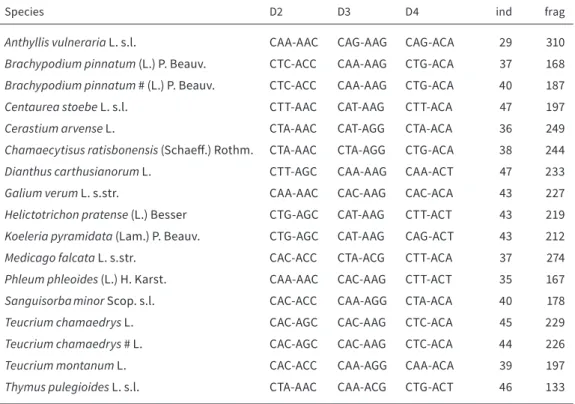
TABLE 2.1 Investigated plant species. Names of the study species, used primer pairs, ind = number of analysed individuals, frag = number of detected fragments. B. pinnatum and T. chamaedrys marked with “#” are repetitions from a second calcareous grassland site
Species D2 D3 D4 ind frag
Anthyllis vulneraria L. s.l. CAA-AAC CAG-AAG CAG-ACA 29 310
Brachypodium pinnatum (L.) P. Beauv. CTC-ACC CAA-AAG CTG-ACA 37 168 Brachypodium pinnatum # (L.) P. Beauv. CTC-ACC CAA-AAG CTG-ACA 40 187
Centaurea stoebe L. s.l. CTT-AAC CAT-AAG CTT-ACA 47 197
Cerastium arvense L. CTA-AAC CAT-AGG CTA-ACA 36 249
Chamaecytisus ratisbonensis (Schaeff.) Rothm. CTA-AAC CTA-AGG CTG-ACA 38 244
Dianthus carthusianorum L. CTT-AGC CAA-AAG CAA-ACT 47 233
Galium verum L. s.str. CAA-AAC CAC-AAG CAC-ACA 43 227
Helictotrichon pratense (L.) Besser CTG-AGC CAT-AAG CTT-ACT 43 219 Koeleria pyramidata (Lam.) P. Beauv. CTG-AGC CAT-AAG CAG-ACT 43 212
Medicago falcata L. s.str. CAC-ACC CTA-ACG CTT-ACA 37 274
Phleum phleoides (L.) H. Karst. CAA-AAC CAC-AAG CTT-ACT 35 167
Sanguisorba minor Scop. s.l. CAC-ACC CAA-AGG CTA-ACA 40 178
Teucrium chamaedrys L. CAC-AGC CAC-AAG CTC-ACA 45 229
Teucrium chamaedrys # L. CAC-AGC CAC-AAG CTC-ACA 44 226
Teucrium montanum L. CAC-ACC CAA-AGG CAA-ACA 39 197
Thymus pulegioides L. s.l. CTA-AAC CAA-ACG CTG-ACT 46 133
ed 20-fold with 1x TE buffer (20 mM Tris-HCl, pH 8.0,
0.1 mM EDTA, pH 8.0). For each tested plant species three primer pairs were selected after executing a primer screening. The chosen primers are shown in Table 2.1. A separate PCR per primer pair was carried out containing 0.75 µl of the diluted pre-selective am- plification product, and in total 4.25 µl of H
2O, 0.25 µM selective MseI (MWG Biotech) primer, 0.05 µM selec- tive EcoRI primer (Proligo, Paris, France), 10x Buffer S, 0.2 mM dNTP and 0.25 U Taq-Polymerase (PeqLab, Erlangen, Germany). To enable a simultaneous detec- tion of resulting fragments the EcoRI primers were labelled, each pair with a different fluorescent dye (Beckmann Coulter, D2, D3, D4). The PCR run includ- ed consecutive steps: initial 2 min at 94 °C, 10 cycles each with denaturation at 94 °C for 0.3 min, annealing starting at 66 °C for 0.5 min and elongation at 72 °C for 2 min. With every cycle passed through the annealing temperature was lowered by 1 °C. Once the 10th cy- cle was finished 25 more iteration with following run parameters were carried out: denaturation at 94 °C for 0.3 min, annealing at 56 °C for 0.5 min and elonga- tion at 72 °C for 2 min. The PCR ended with 30 min at 60 °C and a cool down to 4 °C. For achieving optimal results, the resulting amplified products were diluted differently with 1x TE buffer. 5 µl of each primer pair were mixed and 5 µl stop buffer (Na acetate (3 M, pH 5.2), Na
2EDTA (100 mM, pH 8) and glycogen (20 mgml-1 Roche, Manheim, Germany) at a ratio of 2:2:1) added.
60 µl of 96 % EtOH (4 °C) in combination with shaking causes the precipitation of the DNA and 20 min of cen- trifugation at 14k rpm its aggregation. The superna- tant was removed from the DNA pellet, washed with 200 µl of 76 % ethanol (4 °C) and centrifuged (20 min, 14k rpm) again. After discarding the supernatant, the pellet was dried in a concentrator (Eppendorf concentrator 5301; Eppendorf, Hamburg, Germany).
Prior to the sequencer run, the DNA pellets were dis- solved for 30 min in a mixture of 24.8 µl Sample Load- ing Solution (Beckmann Coulter, USA) and 0.2 µl CEQ Size Standard 400 (Beckmann Coulter, USA). The se- quencer used for fragment detection was a CEQ 8000 (Beckmann Coulter, USA). For every investigated in- dividual we exported the received data into three curve-files, each representing one primer pair. Those virtual gels were analysed manually for the occur- rence of strong, well defined fragments (bands) using Bionumerics 6.6 (Applied Maths, Kortrijk, Belgium).
The presence or absence of bands for every particular fragment size and individual was transformed into a binary (1-0) matrix, which served as basis for all fur- ther analysis. Individuals showing no clear banding signals due to unsuccessful AFLPs were repeated or ultimately excluded.
STATISTICAL ANALYSIS
In total, the AFLP analysis delivered 17 binary matri- ces with a widespread range of detected bands from 133 to 319. For all subsequent calculations of genetic diversities, Nei’s Gene Diversity index (Nei, 1972) was used:
All analyses were conducted either in R 2.15 or when multiple iteration computations were necessary, by a self-developed web-based client/server application, based on Google Web Toolkit (GWT) (Kastlwerk, 2018).
GENE DIVERSITY AND NUMBER OF ANALY- SED FRAGMENTS
In a first step, a possible correlation between the number of detected fragments and Nei’s Gene Diver- sity (He) was investigated. As the result indicated a strong correlation, secondly, in order to analyse all data uniformly, we searched for a threshold beyond which an increasing number of loci would not affect the calculated He of a species. This was done by cal- culating He for each plant species using all available individuals and consecutively changing the number of loci as basis of the computation. The tested loci lev- els were 20, 40, 60, 70, 80, 90, 100, 110, 120, 130, 140, 160, 180, 200, 220 and 240. The loci were randomly selected without allowing duplicates; each step was repeated 10 times and here from one variance-value was calculated. This procedure was rerun 10 times to finally obtain 10 variance-values per fragment level and plant species. All resulting variances of all species and fragment levels were evaluated with a general- ized linear model (McCullagh & Nelder 1989).
GENE DIVERSITY AND NUMBER OF ANALY- SED INDIVIDUALS
Based on the foregoing findings the number of ran- domly selected fragments (m) was set to 120. With this new data set, we repeatedly calculated the Nei’s Gene Diversity (He) for k individuals, with k ranging from two to the maximal number of sampled individ- uals (Table 2.1). The number of repeats (n) was set to 50,000. All 50,000 He values for each k were summa- rised in one mean value:
After that the procedure was rerun 9 times beginning with drawing 120 random fragments. The resulting 10 He values for each number of tested individual and
He = 1 − ∑(𝑝𝑝𝑖𝑖)2
He =∑ Hen i i=1n
12
Chapter 2
each plant species were again summarised in one mean value.
These values were firstly plotted and secondly the best equation describing the obtained non-linear sat- uration curves for every plant species was fitted in R using nls function within the ‘stats’ package (R Core Team, 2013). Therefore, we tested following function types:
root function:
monod hyperbola:
exponential saturation function:
sigmoid function:
and chose the model with the smallest Standard Er- ror of the Regression (S) for further analysis. As the sigmoid function was revealed as best fitting model the function parameters a, b, c were calculated for the existing data (k = 1 to k
max= maximal individuals).
All calculated parameters are shown in Table 2.2.
Moreover, the values from k
100were predicted using the resulting equation. He at a predicted population size of 100 individuals served as default value. Based on this value a 90 % and 95 % He threshold follow- ing Sedcole (1977) was calculated and the associ- ated number of individuals was determined, which therefore represents a minimum sample size (MSS
90, MSS
95). Both collection numbers were tested against each other for significant differentiation via a paired t-test. For a graphical display the saturation curves for every species were plotted using the calculated factors a, b and c. In addition, the confidence inter- vals are shown.
IMPACT OF LIFE HISTORY TRAITS
In order to investigate the influence of life history traits on the resulting MSS we used Pearson’s product moment correlations for following continuous/metric variables ‘canopy height’, ’release height of seeds’,
‘seed mass’, ‘longevity index’, ‘number of dispersal vectors’ and ‘length of flower season’. One-way ANO-
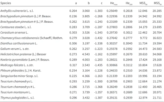
TABLE 2.2 Results of the MSS90 and MSS95 analyses. Investigated plant species (# = species collected on another sample site), calculated factors (a, b, c) for describing a sigmoid equation, Nei’s Gene Diversity calculated with the maximum number of investigated species (=Hemax), the predicted Nei’s Gene Diversity for 100 individuals (=He100), minimum sample size for 90 % (MSS90) respectively 95 % (MSS90) of the predicted Nei’s Gene Diversity.
Species a b c Hemax He100 MSS90 MSS95
Anthyllis vulneraria L. s.l. 0.264 3.060 -1.303 0.25649 0.2618 12.046 20.285 Brachypodium pinnatum (L.) P. Beauv. 0.236 3.805 -1.268 0.22936 0.2339 14.942 24.992 Brachypodium pinnatum # (L.) P. Beauv. 0.262 3.615 -1.243 0.23189 0.2339 15.055 25.333 Centaurea stoebe L. s.l. 0.283 3.709 -1.287 0.27803 0.2806 14.179 23.695
Cerastium arvense L. 0.303 3.526 -1.343 0.29730 0.3012 12.462 20.704
Chamaecytisus ratisbonensis (Schaeff.) Rothm. 0.279 3.028 -1.432 0.27642 0.2777 9.772 16.023 Dianthus carthusianorum L. 0.306 3.197 -1.338 0.30257 0.3040 11.734 19.594
Galium verum L. s.str. 0.262 3.257 -1.223 0.25578 0.2592 14.473 24.583
Helictotrichon pratense (L.) Besser 0.273 4.543 -1.162 0.25997 0.2670 20.610 34.068 Koeleria pyramidata (Lam.) P. Beauv. 0.289 4.003 -1.203 0.28021 0.2848 17.424 29.168 Medicago falcata L. s.str. 0.317 3.543 -1.435 0.30866 0.3112 10.804 17.628 Phleum phleoides (L.) H. Karst. 0.254 3.164 -1.228 0.24633 0.2510 14.036 23.872 Sanguisorba minor Scop. s.l. 0.225 4.366 -1.163 0.21339 0.2203 19.996 33.194
Teucrium chamaedrys L. 0.293 3.259 -1.300 0.28706 0.2903 12.664 21.274
Teucrium chamaedrys # L. 0.286 3.715 -1.368 0.28249 0.2838 12.400 20.465
Teucrium montanum L. 0.271 3.739 -1.357 0.26571 0.2689 12.686 20.971
Thymus pulegioides L. s.l. 0.296 3.432 -1.307 0.29131 0.2939 12.974 21.711
𝑦𝑦 = 𝑎𝑎𝑥𝑥𝑏𝑏
𝑦𝑦 = 𝑎𝑎 × 𝑥𝑥 𝑏𝑏 + 𝑥𝑥
𝑦𝑦 = 𝑎𝑎(1 − 𝑒𝑒𝑏𝑏𝑏𝑏)
𝑦𝑦 = 𝑎𝑎 1 + 𝑏𝑏𝑥𝑥𝑐𝑐 𝑦𝑦 = 𝑎𝑎𝑥𝑥𝑏𝑏
𝑦𝑦 = 𝑎𝑎 × 𝑥𝑥 𝑏𝑏 + 𝑥𝑥
𝑦𝑦 = 𝑎𝑎(1 − 𝑒𝑒𝑏𝑏𝑏𝑏)
𝑦𝑦 = 𝑎𝑎 1 + 𝑏𝑏𝑥𝑥𝑐𝑐 𝑦𝑦 = 𝑎𝑎𝑥𝑥𝑏𝑏
𝑦𝑦 = 𝑎𝑎 × 𝑥𝑥 𝑏𝑏 + 𝑥𝑥
𝑦𝑦 = 𝑎𝑎(1 − 𝑒𝑒𝑏𝑏𝑏𝑏)
𝑦𝑦 = 𝑎𝑎 1 + 𝑏𝑏𝑥𝑥𝑐𝑐 𝑦𝑦 = 𝑎𝑎𝑥𝑥𝑏𝑏
𝑦𝑦 = 𝑎𝑎 × 𝑥𝑥 𝑏𝑏 + 𝑥𝑥
𝑦𝑦 = 𝑎𝑎(1 − 𝑒𝑒𝑏𝑏𝑏𝑏)
𝑎𝑎
VAs were used for the examination of the correlations
of ‘pollination vector’ (wind-pollinated, insect-polli- nated) and the ‘ability to grow clonal’ (yes, no) with MSS. As prerequisite, Nei’s Genetic Diversity (He) val- ues were tested for a correlation with the life history traits to exclude any dependencies. As there could be
another outcome with MSS
90we repeated the tests with those integers and as the results did not differ we excluded them from further analysis (= not shown in this work). The data for all life history traits were taken from two databases, BioPop (Poschlod et al., 2003) and Leda (Kleyer et al., 2008) (Table 2.5).
FIGURE 2.1 Relationships between the number of fragments and the estimated genetic diversity for studied plant species (N = 17).
Pearson correlation: r = 0.372, t-value = 1.552, df = 15, p-value = 0.142
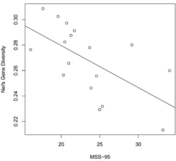
FIGURE 2.2 Relationships between the MSS95 the estimated ge- netic diversity for studied plant species (N = 17). Pearson correlation:
r = -0.602, t value = -2.929, df = 15, p-value = 0.011 *
FIGURE 2.3 Number of fragments plotted against the variance of all in- vestigated species (N = 17).
Chapter 2
●
●
●
●●●●●●●●●●●●●●●●●●●●●●●●●
0 20 40 60 80 100
0.000.050.100.150.200.250.300.35
Anthyllis vulnerariaNumber of Individuals
Nei‘s Gene Diversity
20 Individuals
●
●
●
●
●●●●●●●●●●●●●●●●●●●●●●●●●●●●●●
0 20 40 60 80 100
0.000.050.100.150.200.250.300.35
Phleum phleoides Number of Individuals
Nei‘s Gene Diversity
24 Individuals
●
●
●
●
●
●●●●●●●●●●●●●●●●●●●●●●●●●●●●●●●●●●●●●
0 20 40 60 80 100
0.000.050.100.150.200.250.300.35
Koeleria pyramidataNumber of Individuals
Nei‘s Gene Diversity
29 Individuals
●
●
●
●
●●●●●●●●●●●●●●●●●●●●●●●●●●●●●●●●●●●●●●●●
0 20 40 60 80 100
0.000.050.100.150.200.250.300.35
Teucrium chamaedrysNumber of Individuals
Nei‘s Gene Diversity
21 Individuals
●
●
●
●
●
●●●●●●●●●●●●●●●●●●●●●●●●●●●●●●
0 20 40 60 80 100
0.000.050.100.150.200.250.300.35
Cerastium arvenseNumber of Individuals
Nei‘s Gene Diversity
21 Individuals
●
●
●
●●●●●●●●●●●●●●●●●●●●●●●●●●●●●●●●●
0 20 40 60 80 100
0.000.050.100.150.200.250.300.35
Brachypodium pinnatumNumber of Individuals
Nei‘s Gene Diversity
25 Individuals
●
●
●
●
●●●●●●●●●●●●●●●●●●●●●●●●●●●●●●●●●
0 20 40 60 80 100
0.000.050.100.150.200.250.300.35
Chamaecytisus ratisbonensisNumber of Individuals
Nei‘s Gene Diversity
16 Individuals
●
●
●
●
●●●●●●●●●●●●●●●●●●●●●●●●●●●●●●●●●●●●●●
0 20 40 60 80 100
0.000.050.100.150.200.250.300.35
Helictotrichon pratenseNumber of Individuals
Nei‘s Gene Diversity
34 Individuals
FIGURE 2.4 Display of all investigated plant species. Number of species is drawn against Nei’s Gene Diversity. Measured data of the calculated curves are pictured with a solid black line; predicted data is shown in dashed black. Confidence intervals are given as dashed grey lines. The horizontal dashed grey line gives information about the maximum predicted Nei’s Gene Diversity of 100 individuals (He100) and serves as base for the solid grey line that displays the Nei’s Gene Diversity at a 95 percent level (MSS95). The associated vertical solid grey line marks the intersections with the curve and x-axis and presents the minimum sample size (MSS95).
Anthyllis vulneraria__ Brachypodium pinnatum__
Cerastium arvense__ Chamaecytisus ratisbonensis__
Helictotrichon pratense__ Koeleria pyramidata__
Phleum phleoides__ Teucrium chamaedrys__
●
●
●
●
●●●●●●●●●●●●●●●●●●●●●●●●●●●●●●●●
0 20 40 60 80 100
0.000.050.100.150.200.250.300.35
Medicago falcata Number of Individuals
Nei‘s Gene Diversity
18 Individuals
●
●
●
●●●●●●●●●●●●●●●●●●●●●●●●●●●●●●●●●●●●
0 20 40 60 80 100
0.000.050.100.150.200.250.300.35
Sanguisorba minorNumber of Individuals
Nei‘s Gene Diversity
33 Individuals
●
●
●
●
●●●●●●●●●●●●●●●●●●●●●●●●●●●●●●●●●●
0 20 40 60 80 100
0.000.050.100.150.200.250.300.35
Teucrium montanumNumber of Individuals
Nei‘s Gene Diversity
21 Individuals
●
●
●
●
●●●●●●●●●●●●●●●●●●●●●●●●●●●●●●●●●●●●●●●●●
0 20 40 60 80 100
0.000.050.100.150.200.250.300.35
Thymus pulegioidesNumber of Individuals
Nei‘s Gene Diversity
22 Individuals
●
●
●
●
●
●●●●●●●●●●●●●●●●●●●●●●●●●●●●●●●●●●●●●●●●●
0 20 40 60 80 100
0.000.050.100.150.200.250.300.35
Dianthus carthusianorumNumber of Individuals
Nei‘s Gene Diversity
20 Individuals
●
●
●
●
●●●●●●●●●●●●●●●●●●●●●●●●●●●●●●●●●●●
0 20 40 60 80 100
0.000.050.100.150.200.250.300.35
Brachypodium pinnatum #Number of Individuals
Nei‘s Gene Diversity
25 Individuals ●
●
●
●
●
●●●●●●●●●●●●●●●●●●●●●●●●●●●●●●●●●●●●●●●●●
0 20 40 60 80 100
0.000.050.100.150.200.250.300.35
Centaurea stoebe Number of Individuals
Nei‘s Gene Diversity
24 Individuals
●
●
●
●
●●●●●●●●●●●●●●●●●●●●●●●●●●●●●●●●●●●●●●
0 20 40 60 80 100
0.000.050.100.150.200.250.300.35
Galium verum Number of Individuals
Nei‘s Gene Diversity
25 Individuals
●
●
●
●
●●●●●●●●●●●●●●●●●●●●●●●●●●●●●●●●●●●●●●●
0 20 40 60 80 100
0.000.050.100.150.200.250.300.35
Teucrium chamaedrys #Number of Individuals
Nei‘s Gene Diversity
20 Individuals
Brachypodium pinnatum #__ Centaurea stoebe__
Dianthus carthusianorum__ Galium verum__
Medicago falcata__ Sanguisorba minor__
Teucrium chamaedrys #__
Thymus pulegioides__
Teucrium montanum__
Chapter 2
2.3 RESULTS
GENE DIVERSITY AND NUMBER OF ANALY- SED FRAGMENTS
The number of detected fragments ranged from 133 for Thymus pulegioides to 319 for Anthyllis vuleraria.
Although Figure 2.1 appears to show a correlation be- tween the number of detected loci and the height of Nei’s Gene Diversity (He), this result was not statisti- cally significant (p = 0.142, t = 1.552, r = 0.372).
As Figure 2.2 shows, MSS
95was significantly corre- lated with He (p = 0.011, t = -2.929, r = -0.602). The same applied for MSS
90(p = 0.013, t = -2.815, r = -0.588).
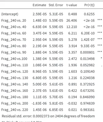
The analysis of the different variances for the test- ed numbers of loci showed that the minimum number of fragments to estimate genetic diversity was 120.
Below this threshold, the fluctuation of the calculat- ed data had a significant influence on the variance of the data and therefore on He. Above this value, there was no significant difference to the maximum He
max(Figure 2.3, Table 2.3).
GENE DIVERSITY AND NUMBER OF ANALY- SED INDIVIDUALS
The run of the sigmoid saturation curves showed that the different number of sampled individuals had a clear impact on the maximum measured Nei’s Gene Diversity (He
max). For most of the tested species like Chamaecytisus ratisbonensis or Anthyllis vulnerar- ia, the curves showed a steep ascending slope for a sample size between 2 and 15. On the other hand we also detected flat inclinations for species like He- lictotrichon pratense or Koeleria pyramidata. In the subsequent development, the curves plateaued. The sigmoid curve consisted of three factors a, b, c. While a describes the maximum possible genetic variation of the tested species, both remaining factors b and c together define the steepness of the curves progres- sion. The smaller b and c, the steeper the slope, i.e.
the faster MSS
95is reached (Figure 2.4).
The values for MSS
95were significantly higher than for MSS
90(p < 0.0001, t = -19.323). The calculat- ed values ranged from a minimum of MSS
90= 9.77 respectively MSS
95= 16.02 for Chamaecytisus ratis- bonensis to a maximum of MSS
90= 20.61 respectively MSS
95= 34.07 for Helictotrichon pratense. The mean value for a minimum sample size including all spe- cies is 14.0 for a 90 % coverage of the population’s estimated total Gene Diversity (= MSS
90) and 23.4 for a 95 % coverage (= MSS
95), respectively. The highest measured Nei’s Gene Diversity (He) with 48 investi- gated individuals had Medicago falcata with 0.309, the lowest value had Sanguisorba minor (40 tested individuals) with 0.213. The mean calculated He for all species was 0.268. It is worth mentioning that the repeated collection of the two species Brachypodium pinnatum and Teucrium chamaedrys at different field sites did not influence the MSS
90, which is 14.94 vs.
15.06 for Brachypodium pinnatum e.g. 12.66 vs. 12.40 for Teucrium chamaedrys. Figure 2.4 shows He values which were plotted against the gradually increasing number individuals and the fitted curves for each species. The related factors a, b, c and the expect- ed maximum Nei’s Gene Diversity (He
100= calculated Nei’s Gene Diversity for 100 individuals) compared to the He
max(calculated value with the all sampled individuals per species) are shown in Table 2.2. Both values, He
max(p = 0.011, t = -2.919, r = -0.602) and He
100(p = 0.014, t = -2.781, r = -0.583) correlated significantly with MSS
95, showing a negative dependency between the minimum sample size and the height of He. On the other hand, MSS
95did not depend on the total num- ber of tested individuals (p-value = 0.498, t = 0.694, r = 0.176).
Estimate Std. Error t-value Pr(>|t|) (Intercept) 2.59E-05 5.31E-05 0.488 0.6255 Frag_240 vs. 20 1.48E-03 5.59E-05 26.406 < 2e-16 ***
Frag_240 vs. 40 6.83E-04 5.59E-05 12.210 < 2e-16 ***
Frag_240 vs. 60 3.47E-04 5.59E-05 6.211 6.20E-10 ***
Frag_240 vs. 70 2.95E-04 5.59E-05 5.278 1.42E-07 ***
Frag_240 vs. 80 2.19E-04 5.59E-05 3.914 9.33E-05 ***
Frag_240 vs. 90 1.88E-04 5.59E-05 3.357 0.000801 ***
Frag_240 vs.100 1.38E-04 5.59E-05 2.472 0.013498 * Frag_240 vs. 110 1.08E-04 5.59E-05 1.936 0.052982 . Frag_240 vs. 120 8.96E-05 5.59E-05 1.603 0.109140 Frag_240 vs. 130 6.80E-05 5.59E-05 1.216 0.224038 Frag_240 vs. 140 5.00E-05 5.61E-05 0.891 0.372925 Frag_240 vs. 160 2.37E-05 5.61E-05 0.422 0.673291 Frag_240 vs. 180 1.11E-05 5.70E-05 0.194 0.846090 Frag_240 vs. 200 -1.83E-06 5.81E-05 -0.032 0.974839 Frag_240 vs. 220 1.45E-06 6.85E-05 0.021 0.983161 Residual std. error: 0.0002373 on 2404 degrees of freedom Multiple R-squared:0.724
TABLE 2.3 Output of a generalized linear model. Results of a GLM in which the differentiation of the variance of the maximum num- ber of detected fragments (240) was tested against different frag- ment-levels (20 - 220). Up to 100 fragments there was a significant difference in the variance noticeable and also 110 fragments dis- played a tendency. Using 120 fragments or more showed no signif- icant difference between the maximum fragment variance and the tested fragment-level.
PLANT FUNCTIONAL TRAITS CORRELATE WITH MSS BUT NOT WITH NEI’S GENE DI- VERSITY
The investigation of a possible relation between the minimum sample size (MSS) and life history traits revealed only one trait with a significant correlation.
The pollination type correlated significantly with MSS
90(r = 0.75, p = 0.0003, Table 2.4) and MSS
95(r = 0.76, p = 0.0002, Table 2.4). In both cases insect-pollinated species had a significantly lower MSS (MSS
90with 12.381 ± 0.40 SE, MSS
95with 20.630 ± 0.73 SE) than wind-pollinated plants where 17.011 ± 1.14 SE (MSS
90) and 28.438 ± 1.80 SE (MSS
95) individuals must be col- lected to reach 95 % of the total Nei’s Gene Diversi- ty. Insect-pollinated species had higher measure- ments of Nei’s Gene Diversities (0.28 ± 0.01 SE) than wind-pollinated species (0.24 ± 0.02 SE), but like all other tested life history traits, this difference was not significant (Table 2.4).
2.4 DISCUSSION
In this study we analysed how many loci and individu- als are needed for a stable determination of 90 % and 95 % of the total genetic diversity of a plant popula- tion. In this way, we wanted to contribute to a more efficient use of the financial resources available for the analysis of genetic diversity.
In order to determine the adequate number of in- dividuals, it was necessary to specify the number of fragments, which are required to capture most of a population’s genetic diversity. Simulations of Mari- ette et al. (2002) showed that AFLP markers produce good estimates of genetic variation at whole genome level, but when migration rates are higher and popu- lations exhibit low genomic heterogeneities, at least ten times more markers are necessary to reach the ef- ficiency of microsatellites to predict the whole genet- ic diversity. The results for our 15 surveyed calcareous grassland species showed that reaching a number of 120 fragments (poly- and monomorphic) is sufficient to estimate a population’s genetic diversity via AFLPs.
Beyond this threshold, additional fragments did not significantly increase the estimates of genetic diver- sity. Fewer than 120 fragments resulted in significant- ly lower estimates of genetic diversity and therefore increased the probability of not embracing the total
TABLE 2.4 Analyses of variance conducted with different life history traits as responsive variables. Number of studies in each group (n), mean values, standard derivation (SD), t-values, residual standard errors, degrees of freedom, p-values, Fstat and adjusted r are given.
n mean SD t-value Residual SD error
degrees of freedom
p-value Fstat r
MSS90
Pollination vector 1,949 15 0.0003 21,91 0.75
Insect 11 12,381 0,590 21,074
Wind 6 17,011 0,990 4,681
MSS95
Pollination vector 3.219 15 0.0002 22.84 0.76
Insect 11 20.631 0.947 21.258
Wind 6 28.438 1.634 4.779
Clonality 5.070 15 0.6230 0.25 0.13
yes 8 24.041 1.793 13.412
no 9 22.804 2.464 -0.502
Canopy height 17 0.497 1.373 15 0.1900 0.33
Release height 17 0.559 1.622 15 0.1256 0.39
Seedmass 17 2.009 0.965 15 0.3501 0.24
Longevity index 17 0.093 -0.522 10 0.6133 -0.16
Dispersal vectors 17 2.846 0.899 11 0.3880 0.26
Flower duration 17 3.000 0.273 15 0.7890 0.07
Chapter 2
Except for Sanguisorba minor , the majority of our in- vestigated wind-pollinated species were grasses.
Considering the pollination vector the referred study divided their surveyed species into three groups with an additional category self-pollinated and found no clear results, which was explained by the difficult designation of the species’ pollination vectors. This contradiction may be explained by different sample designs of the studies. Most of the surveyed articles had a large-scaled focus with a mean distance be- tween the populations of 1,513 ± 2,529 km. We on the other hand tested individuals on a small scale of 440 meters, with an emphasis on the genetic variation within the population of a species. From this point of view, a lower genetic variation of wind-pollinat- ed plants can be expected due to the fact, that pol- len transported via wind can bridge larger distances between the individuals of one population than be- tween insect-pollinated plant individuals. Therefore genetic differentiation of wind-pollinated individuals can be considered smaller, i.e. the individuals of this population are more genetically homogeneous. On the other hand we would predict insect-pollinated plants to display a higher genetic heterogeneity with- in the population because of a smaller transportation vector and a higher selectivity of the pollinators. As genetic variability rises with the number of different tested individuals, for a genetically homogeneous population a higher sample size has to be collected to gain 95 % of the total genetic variation. The homoge- ny leads to the fact that more individuals need to be collected over the whole population to sufficiently characterize the genetic variation.
CONCLUSIONS
Our findings demonstrate that on the whole, in most studies a sufficient number of individuals or rather just as many individuals have been used for the esti- mation of genetic variation resulting in diversity val- ues located on the plateau of the progression curves.
We therefore emphasise that there is no need to fol- low the trend to increase sample sizes, as it is an un- necessary expense in time and money. Financial re- sources should instead better used to analyse further populations or species.
population’s genetic variation. This perfectly fits the results of Mittell et al. (2015) who showed that the me- dian of 10 microsatellite loci currently used in genetic studies is sufficient for characterising a population’s molecular genetic variation.
Based on these findings, we investigated our sec- ond question concerning the sufficient number of in- dividuals to satisfactorily characterize and compare the genetic diversity of populations. To exclude bias of fragment detection, we randomly chose 120 frag- ments each for all following tests. The results showed that He followed a non-linear saturation curve, which ascended steeply with sample size until a plateau was reached. In other words, the curve progression culminated in a saturation point beyond which an in- creased sample size had no significant influence on the genetic variation estimated from the total popu- lation sample. Our compilation of 15 different calcar- eous grassland species revealed that an overall mean of 23.4 ± 1.20 randomly chosen individuals per pop- ulation were sufficient to cover 95 % of the total ge- netic variance. Interestingly, similar results have been reported for other organisms such as lichens (Werth, 2011) or birds (Pruett & Winker, 2008). Our results were also corroborated by the work of McGlaughlin et al.
(2015). The authors of this study determined a range of 10 to 30 individuals necessary to capture 90 % of the genetic variation estimated from the total pop- ulation sample of an endangered Californian plant species, which matches with our observations. Fewer individuals are required to estimate diversity when diversity is great (t = -2.919, df = 15, p-value = 0.011, r = -0.602). But neither MSS nor He was dependent on the initial total number of individuals (population size). This supports the results of the review of Reisch and Bernhardt-Römermann (2014) who showed that genetic variation was independent from sample size and who concluded that the number of individuals did not influence the outcome of study comparisons.
Pollination type was the only life history trait
that was significantly correlated with MSS
95(r = 0.78,
p = 0.0002). In order to characterize the genetic var-
iation of wind pollinated plants, more individuals
had to be collected than for insect pollinated species
(MSS
90with 17.0 ± 1.1 SE individuals vs. 12.4 ± 0.4 SE,
MSS
9528.4 ± 1.8 SE individuals vs. 20.6 ± 0.7 SE). Curve
progressions in the two categories were almost con-
stantly different with insect pollinated plants showing
higher values of genetic variation and a steeper curve
progression than wind pollinated plants. However,
He was not significantly different. This can be relat-
ed to the findings of Reisch & Bernhardt-Römermann
(2014) who also had non-significant but higher genetic
variations for dicotyledons than for monocotyledons.
APPENDIX
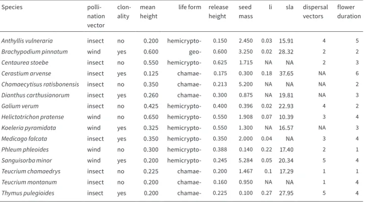
TABLE 2.5 List of studied plant species and plant traits (- = phyte): li = longevity index, sla = specific leaf area.
Species polli-
nation vector
clon- ality
mean height
life form release height
seed mass
li sla dispersal vectors
flower duration
Anthyllis vulneraria insect no 0.200 hemicrypto- 0.150 2.450 0.03 15.91 4 5
Brachypodium pinnatum wind yes 0.600 geo- 0.600 3.250 0.02 28.32 2 2
Centaurea stoebe insect no 0.550 hemicrypto- 0.625 1.715 NA NA 2 3
Cerastium arvense insect yes 0.125 chamae- 0.175 0.300 0.18 37.65 NA 6
Chamaecytisus ratisbonensis insect no 0.350 chamae- 0.213 5.200 NA NA NA 2
Dianthus carthusianorum insect yes 0.260 chamae- 0.300 0.875 NA 19.81 NA 3
Galium verum insect no 0.425 hemicrypto- 0.400 0.396 0.02 22.93 4 2
Helictotrichon pratense wind no 0.650 hemicrypto- 0.550 1.908 0.07 10.39 3 4
Koeleria pyramidata wind yes 0.325 hemicrypto- 0.550 1.300 NA 16.57 NA 3
Medicago falcata insect yes 0.350 hemicrypto- 0.350 2.000 0.04 NA 3 4
Phleum phleoides wind no 0.300 hemicrypto- 0.388 0.140 0.22 17.40 2 1
Sanguisorba minor wind yes 0.200 hemicrypto- 0.245 5.284 0.05 20.34 5 4
Teucrium chamaedrys insect no 0.225 chamae- 0.200 1.467 0.1 17.29 1 1
Teucrium montanum insect no 0.200 chamae- 0.160 0.950 NA NA 1 4
Thymus pulegioides insect yes 0.200 chamae- 0.225 0.100 0.27 27.95 5 4