Customizable Route Planning in Road Networks

Customizable Route Planning in Road Networks

Daniel Delling¹, Andrew V. Goldberg¹, Thomas Pajor², and Renato F. Werneck¹

1 Microsoft Research Silicon Valley {dadellin,goldberg,renatow}@microsoft.com

2 Karlsruhe Institute of Technology pajor@kit.edu

July 24, 2013

Abstract. We propose the first routing engine for computing driving directions in large-scale road networks that satisfies all requirements of a real-world production system. It supports arbitrary metrics (cost functions) and turn costs, enables real-time queries, and can incorporate a new metric in less than a second, which is fast enough to support real-time traffic updates and personalized cost functions. The amount of metric-specific data is a small fraction of the graph itself, which allows us to maintain several metrics in memory simultaneously. The algorithm is the core of the routing engine currently in use by Bing Maps.

1 Introduction

A key ingredient of modern online map applications is a routing engine that can find best routes between two given location of a road network. This task can be translated into finding point-to-point shortest paths in a graph representing the road network. Although the classic algorithm by Dijkstra [25] runs in almost linear time with very little overhead, it still takes a few seconds on continental-sized graphs. This has motivated a large amount of research (see [19] or [62] for overviews) on speedup techniques that divide the work in two phases:preprocessing takes a few minutes (or even hours) and produces a (limited) amount of auxiliary data, which is then used to perform queries in a millisecond or less. Most previous research has been evaluated on benchmark data representing simplified models of the road networks of Western Europe and the United States, using the most natural metric, driving times, as the optimization function. The fastest technique, called HL [1, 2], can compute the driving time between any two points in a few hundred nanoseconds, or millions of times faster than Dijkstra’s algorithm. Unfortunately, using such techniques in an actual production system is far more challenging than one might expect.

An efficient real-world routing engine must satisfy several requirements. First, it must incorporate all details of a road network—simplified models are not enough. In particular, previous work often neglected turn costs and restrictions, since it has been widely believed that any algorithm can be easily augmented to handle these efficiently. We show that, unfortunately, most methods actually have a significant performance penalty, especially if turns are represented space-efficiently. Moreover, a practical algorithm should be able to handle other natural metrics (cost functions) besides travel times, such as shortest distance, walking, biking, avoid U-turns, avoid/prefer freeways, avoid left turns, avoid ferries, and height and weight restrictions. In fact, the routing engine should provide reasonable performance guarantees for any metric, thus enabling personalized driving directions with no risk of timeouts. To support multiple cost functions efficiently, the algorithm should store as little data per metric as possible. In addition, new metrics should be incorporated quickly, thus enabling real-time traffic information to be part of the cost function. Moreover, updates to the traversal cost of a small number of road segments (due to road blocks, for example) should be handled even more efficiently. The engine should support not only the computation of point-to-point shortest paths,

?This is the full version of two conference papers [15, 22]. This work was done while the third author was at Microsoft Research Silicon Valley.

but also extended query scenarios, such as alternative routes. Finally, the routing engine should not be the bottleneck of a map application. All common types of queries should run in real time, i.e., fast enough for interactive applications.

In this paper, we report our experience in building a routing engine that meetsall the above-mentioned requirements for a modern map server application. Surprisingly, the work goes far beyond simply implement- ing an existing technique in a new scenario. It turns out that no previous technique meets all requirements:

Even the most promising candidates fail in one or more of the critical features mentioned above. We will argue that methods with a strong hierarchical component, the fastest in many situations, are too sensitive to metric changes. We choose to focus on separator-based methods instead, since they are much more robust.

Interestingly, however, these algorithms have been neglected in recent research, since previously published results made them seem uncompetitive. The highest reported speedups [39] over Dijkstra’s algorithm were lower than 60, compared to thousands or millions with other methods. By combining new concepts with careful engineering, we significantly improve the performance of this approach, easily enabling interactive applications.

One of our main contributions is the distinction betweentopologicalandmetricproperties of the network.

Thetopologyis the graph structure of the network together with a set of static properties of each road segment or turn, such as physical length, number of lanes, road category, speed limit, one- or two-way, and turn types.

Themetricencodes the actual cost of traversing a road segment or taking a turn. It can often be described compactly, as a function that maps (in constant time) the static properties of an arc/turn into a cost. For example, in thetravel timemetric (assuming free-flowing traffic), the cost of an arc may be its length divided by its speed limit. We assume the topology is shared by the metrics and rarely changes, while metrics may change quite often and can even be user-specific.

To exploit this separation, we consider algorithms for realistic route planning withthree stages. The first, metric-independent preprocessing, may be relatively slow, since it is run infrequently. It takes only the graph topology as input, and may produce a fair amount of auxiliary data (comparable to the input size). The second stage,metric customization, is run once for each metric, and must be much quicker (a few seconds) and produce little data—a small fraction of the original graph. Finally, the query stage uses the outputs of the first two stages and must be fast enough for real-time applications. We call the resulting approach Customizable Route Planning (CRP).

We stress that CRP is not meant to compete with the fastest existing methods on individual metrics. For

“well-behaved” metrics (such as travel times), our queries are somewhat slower than the best hierarchical methods. However, CRP queries are robust and suitable for real-time applications with arbitrary metrics, including those for which the hierarchical methods fail. CRP can process new metrics very quickly (orders of magnitude faster than any previous approach), and the metric-specific information is small enough to allow multiple metrics to be kept in memory at once. We achieve this by revisiting and thoroughly reengineering known acceleration techniques, and combining them with recent advances in graph partitioning.

This paper is organized as follows. In Section 2 we formally define the problem we solve, and explore the design space by analyzing the applicability of existing algorithms to our setting. Section 3 discusses overlay graphs, the foundation of our approach. We discuss basic data structures and modeling issues in Section 4.

Our core routing engine is described in Section 5, with further optional optimizations discussed in Section 6.

In Section 7 we present an extensive experimental evaluation of our method, including a comparison with alternative approaches. Section 8 concludes with final remarks.

2 Framing the Problem

This section provides a precise definition of the basic problem we address, and discusses potential approaches to solve it.

Formally, we consider a graphG= (V, A), with a nonnegativecost function `(v, w) associated with each arc (v, w) ∈ A. Our focus is on road networks, where vertices represent intersections, arcs represent road segments, and costs are computed from the properties of the road segments (e.g., travel time or length).

A path P = (v0, . . . , vk) is a sequence of vertices with (vi, vi+1) ∈ A, and its cost is defined as `(P) =

Pk−1

i=0 `(vi, vi+1). The basic problem we consider is computing point-to-point shortest paths. Given a source s and a target t, we must find the distance dist(s, t) between them, defined as the length `(Opt) of the shortest pathOpt inGfromstot. We will ignore turn restrictions and turn costs for now, but will discuss them in detail in Section 4.1.

This problem has a well-known solution: Dijkstra’s algorithm [25]. It processes vertices in increasing order of distance froms, and stops whentis reached. Its running time depends on the data structure used to keep track of the next vertex to scan. It takes O(m+nlogn) time (with n=|V| and m=|A|) with Fibonacci heaps [28], orO(m+nlogC/log logC) time with multilevel buckets [24], which is applicable when arc lengths are integers bounded byC. In practice, the data structure overhead is quite small, and the algorithm is only two to three times slower than a simple breadth-first search [34]. One can save time by running a bidirectional version of the algorithm: in addition to running a standardforward search froms, it also runs areverse (or backward) search fromt. It stops when the searches meet.

On continental road networks, however, even carefully tuned versions of Dijkstra’s algorithm would still take a few seconds on a modern server to answer a long-range query [56, 14]. This is unacceptable for interac- tive map services. Therefore, in practice one must rely on speedup techniques, which use a (relatively slow) preprocessing phase to compute additional information that helps accelerate queries. There is a remarkably wide selection of such techniques, with different tradeoffs between preprocessing time, space requirements, query time, and robustness to metric changes. The remainder of this section discusses how well these tech- niques fit the design goals set forth in Section 1. Recall that our main design goals are as follows: we must support interactive queries onarbitrary metrics, preprocessing must be quick (a matter of seconds), and the additional space overhead per cost function should be as small as possible.

Some of the most successful existing methods—such as reach-based routing [36], contraction hierar- chies [32], SHARC [10], transit node routing [6, 5, 55, 4], and hub labels [1, 2, 17]—rely on the stronghierarchy of road networks with travel times. Intuitively, they use the fact that shortest paths between vertices in two faraway regions of the graph tend to use the same major roads.

The prototypical method among these is contraction hierarchies (CH). During preprocessing, CH heuris- tically sorts the vertices in increasing order of importance, and shortcuts them in this order. (Toshortcut v, one temporarily removes it from the graph and adds as few arcs between its neighbors as necessary to preserve distances.) Queries run bidirectional Dijkstra, but only follow arcs or shortcuts to more important vertices. This rather simple approach works surprisingly well. On a continental-sized road network with tens of millions of vertices, using travel times as cost function (but ignoring turn costs), preprocessing is a matter of minutes, and queries visit only a few hundred vertices, resulting in query times well below 1 ms.

For metrics that exhibit strong hierarchies, such as travel times, CH has many of the features we want.

Queries are sufficiently quick, and preprocessing is almost fast enough to enable real-time traffic. Moreover, Geisberger et al. [32] show that if a metric changes only slightly (as in most traffic scenarios), one can keep the order and recompute the shortcuts in about a minute on a standard server. Unfortunately, an order that works for one metric may not work for a substantially different metric (e.g., travel times and distances). Fur- thermore, queries are much slower on metrics with less-pronounced hierarchies [11]. For instance, minimizing distances instead of travel times leads to queries up to 10 times slower. This does not render algorithms such as CH impractical, but one should keep in mind that the distance metric is still far from the worst case. It still has a fairly strong hierarchy: since major freeways tend to be straighter than local roads, they are still more likely to be used by long shortest paths. Other metrics, including some natural ones, are less forgiving, in particular in the presence of turns. More crucially, the preprocessing stage can become impractical (in terms of space and time) for bad metrics, as Section 7 will show.

Other techniques, such as PCD [48], ALT [35], and arc flags [38, 45], are based on goal direction, i.e., they try to reduce the search space by guiding the search towards the target. Although they produce the same amount of auxiliary data for any metric, queries are not robust, and can be as slow as Dijkstra for bad metrics. Even for travel times, PCD and ALT are not competitive with other methods.

A third approach is based on graph separators [42, 60, 43, 61, 39]. During preprocessing, one computes a multilevel partition of the graph to create a series of interconnectedoverlay graphs (smaller graphs that preserve the distances between a subset of the vertices in the original graph). A query starts at the lowest

(local) level and moves to higher (global) levels as it progresses. These techniques, which predate hierarchy- based methods, have been widely studied, but recently dismissed as inadequate. Their query times are generally regarded as uncompetitive in practice, and they have not been tested on continental-sized road networks. The exceptions are recent extended variants [18, 52]; they achieve good query times, but only by adding many more arcs during preprocessing, which is costly in time and space. Despite these drawbacks, the fact that preprocessing and query times are essentially metric-independent makes separator-based methods the most natural fit for our problem.

There has also been previous work on variants of the route planning problem that deal with multiple metrics in a nontrivial way. The preprocessing of SHARC [10] can be modified to handle multiple (known) metrics at once. In theflexible routing problem [30, 29], one must answer queries on linear combinations of a small set of metrics (typically two or three) known in advance. Geisberger et at. [31] extend this idea to handle a predefined set of constraints on arcs, which can be combined at query time to handle scenarios like height and weight restrictions. Delling and Wagner [20] consider multicriteria optimization, where one must find Pareto-optimal paths among multiple metrics. ALT [35] and CH [32] can adapt to small changes in a benign base metric without rerunning preprocessing in full. All these approaches must know the base metrics in advance, and for good performance the metrics must be few, well-behaved, and similar to one another. In practice, even seemingly small changes to the metric (such as moderate U-turn costs) render some approaches impractical. In contrast, we must process metrics as they come (in the presence of traffic jams, for instance), and assume nothing about them.

3 Overlay Graphs

Having concluded that separator-based techniques are the best fit for our requirements, we now discuss this approach in more detail. In particular, we formally define partitions and revisit the existing technique of partition-based overlay graphs and its variants, with emphasis on how it fits our purposes.

3.1 Partitions

A partition of V is a family C={C0, . . . , Ck} of cells (sets)Ci ⊆V with eachv ∈V contained in exactly one cellCi. LetU be the size (number of vertices) of the biggest cell. A multilevel partition ofV is a family of partitions{C⁰, . . . ,C^L}, whereldenotes thelevel of a partitionC^landU^lrepresents the size of the biggest cell on level l. We set U⁰ = 1, i.e., the level 0 contains only singletons. To simplify definitions, we also set C^L+1=V. Throughout this paper, we only usenested multilevel partitions, i.e., for eachl≤Land each cell C_i^l∈ C^l, there exists a cellC_j^l+1 ∈ C^l+1 (called the supercell of C_i^l) withC_i^l⊆C_j^l+1. Conversely, we call C_i^l asubcell ofC_j^l+1 ifC_j^l+1 is the supercell ofC_i^l. Note that we denote byLthe number of levels and that the supercell of a level-Lcell isV. We denote by cl(v) the cell that containsv on levell. To simplify notation, whenL= 1 we may use c(v) instead of c1(v). Aboundary (orcut) arc on levell is an arc with endpoints in different level-l cells; aboundary vertex on levell is a vertex with at least one neighbor in another level-l cell. Note that, for nested multilevel partitions, boundary arcs are nested as well: a boundary arc at levell is also a boundary arc on all levels below.

3.2 Basic Algorithm

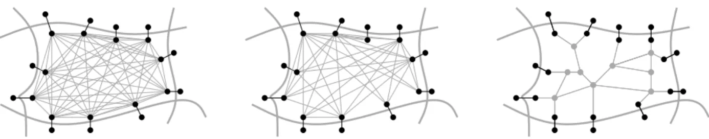
The preprocessing of the partition-based overlay graphs speedup technique [60] first finds a partition of the input graph and then builds a graph H containing all boundary vertices and boundary arcs of G. It then builds aclique for each cellC: for every pair (v, w) of boundary vertices inC, it creates an arc (v, w) whose cost is the same as the shortest path (restricted toC) betweenv andw(or infinity ifwis not reachable from v using only arcs inC). See Fig. 1. One can determine the costs of theseshortcut arcs by running Dijkstra from each boundary vertex.

Theorem 1. H is an overlay of G.

Fig. 1.Three possible ways of preserving distances within the overlay graph. Storing full cliques (left), performing arc reduction on the clique arcs (middle), and storing a skeleton (right).

Proof. For any two verticesu, vinH, we must show that the distance between them is the same inGandH (i.e., thatdistG(u, v) =distH(u, v)). By construction, every arc we add toH corresponds to a path of equal cost inG, sodH(u, v)≥dG(u, v) for allu, v∈H (distances cannot decrease). Consider the shortest pathPuv

betweenuandv in G. It can be seen a sequence of subpaths between consecutive boundary vertices. Each of these subpaths is either a boundary arc (which belongs toH by construction) or a (shortest) path within a cell between two boundary vertices (which corresponds to a shortcut arc inH, also by construction). This means there is au–vpath inH with the same cost asPuv, ensuring thatdH(u, v)≤dG(u, v) and concluding our proof.

Note that the theorem holds even though some shortcuts added toH are not necessarily shortest paths in eitherGorH. Such shortcuts are redundant, but do not affect correctness.

To perform a query betweensandt, one runs a bidirectional version of Dijkstra’s algorithm on the graph consisting of the union of H, c(s), and c(t), called the search graph. The fact that H is an overlay of G ensures queries are correct, as shown by Holzer et al. [39]. Intuitively, consider the shortest path inGfrom stot. It consists of three parts: a maximal prefix entirely inc(s), a maximal suffix entirely inc(t), and the remaining “middle” part. By construction, the segments inc(s) andc(t) are part of the search space, and the overlay H contains a path of equal cost as the path representing the middle part, with the same start and end vertex. Since the overlay does not decrease the distances between any two vertices, we find a path of equal cost to the shortest inG.

To accelerate queries, partition-based approaches often use multiple levels of overlay graphs. For each level i of the partition, one creates a graph Hi as before: it includes all boundary arcs, plus an overlay linking the boundary vertices within a cell. If one builds the overlays in a bottom-up fashion, one can use H_i−1 (instead ofG) when running the Dijkstra searches from the boundary vertices ofHi. This accelerates the computation of the high-level overlay graphs significantly. During queries, we can skip cells that contain neithersnort. More precisely, ans–tquery runs bidirectional Dijkstra on a restricted search graphGst. An arc (v, w) from Hi will be inGst if both v and w are in the same cell as s or t on leveli+ 1, but not on leveli.

3.3 Pruning the Overlay Graph

The basic overlay approach stores a full clique per cell for each metric, which seems wasteful. Many shortcuts are not necessary to preserve the distances within the overlay graph because the shortest path between their endpoints actually uses some arcs outside the cell. (These shortcuts are introduced because construction considers only paths within a cell.) This happens particularly often for well-behaved metrics. A first approach to identify and remove such arcs isarc reduction [60]. After computing all cliques, Dijkstra’s algorithm is run from each vertexuin H, stopping as soon as all neighbors of v (in H) are scanned. Then, one can remove all arcs (u, v) fromH withdist(u, v)< `(u, v). These searches are usually quick (they only visit the overlay), and we can avoid pathological cases by having a hard bound on the size of the search space. Although this can miss some opportunities for pruning, it preserves correctness.

A more aggressive technique to further reduce the size of the overlay graph is to preserve some internal cell vertices [61, 39, 18]. IfB ={v1,v2,. . .,vk}is the set of boundary vertices of a cell, letTibe the shortest path tree (restricted to the cell) rooted at vi, and letT_i⁰ be the subtree ofTi consisting of the vertices with descendants inB. One can take the union S =∪^k_i=1T_i⁰ of these subtrees, and shortcut all internal vertices with two neighbors or fewer. We call the resulting object a skeleton graph; it is technically not an overlay, since the distances between its internal vertices may not be preserved. But it does preserve the distances between allboundary vertices, which is enough to ensure correctness [39]. Both arc reduction and skeletons can be naturally extended to work with multiple levels of overlay graphs. In Section 5.4, we will discuss which of these optimizations carry over to a realistic routing environment.

4 Modeling

The first step for building a fully-fledged routing engine is to incorporate all modeling constraints, such as turn restrictions and turn costs. Moreover, we want to be able to handle multiple metrics without explicitly storing a traversal cost for each arc and metric. In this section, we explain the data structures we use to support these two requirements and show how Dijkstra’s algorithm can be adapted. These are both building blocks to the fast routing engine we will present in Section 5.

4.1 Turns

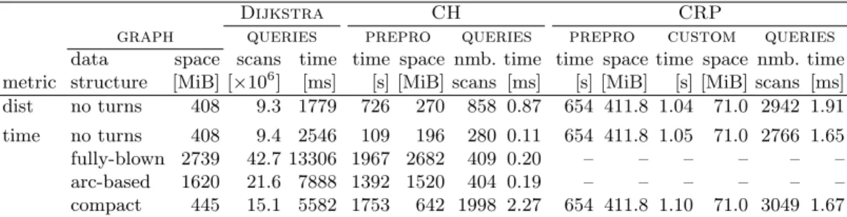
Most previous work on route planning algorithms has considered a simplified representation of road networks, with each intersection corresponding to a single vertex (see Fig. 2). This is not enough for a real-world production system, since it does not account for turn costs (or restrictions, a special case). In principle, any algorithm can handle turns simply by working on an expanded graph. The most straightforward approach is to introduce two vertices, a head vertex and a tail vertex per directed arc. Tail and head vertices are connected as before by a road arc. In addition,turn arcs model allowed turns at an intersection by linking the head vertex of an arc to the tail vertex of another. This fully-blown approach is wasteful, however; in particular, tail vertices now always have out-degree 1 and head vertices have in-degree 1. A slightly more compact representation is arc-based: one only keeps the tail vertices of each intersection, and each arc is a road segment followed by a turn.

To save even more space, we propose acompact representationin which each intersection becomes a single vertex with some associated information. If a vertexuhaspincoming andq outgoing arcs, we associate a p×qturn tableTuto it, whereTu[i, j] represents the cost of turning from thei-th incoming arc into thej-th outgoing arc at u. In addition, we store with each arc (v, w) itstail order (its position amongv’s outgoing arcs) and itshead order (its position amongw’s incoming arcs). These orders may be arbitrary. Since degrees are small in practice, 8 bits for each suffice. For each arc (u, v), we say that its head corresponds to anentry point at v, and its tail corresponds to an exit point atu. Note that the entry/exit points translate directly to the head/tail vertices in the fully blown model.

In practice, many vertices tend to share the same turn table. The total number of suchintersection types is modest—in the thousands rather than millions. For example, many degree-four vertices in the United

Fig. 2.Turn representations (from left): none, fully expanded, arc-based, and compact.

States have four-way stop signs with exactly the same turn costs. Each distinct turn table is thus stored only once, and each vertex keeps a pointer to the appropriate type, with little overhead.

Finally, we note that data representing real-world road networks often comes with so-calledpolyvalent turn restrictions, as observed before [58, 59]. Depending on which turn a driver takes at a particular intersection, certain turns may be forbidden at the next. For example, if one turns right onto a multilane street, one is often forbidden to take a left exit that is just a few meters ahead. Drivers who are already in the multilane street have no such constraint. Such (rare) scenarios can be handled by locally “blowing up” the graph with additional arcs and/or vertices for each affected intersection. In this example, representing this segment of the multilane street by two (parallel) arcs is enough to accurately represent all valid paths. On our proprietary data, the number of such polyvalent turns is very small, and thus the size of the routing graph increases only slightly.

4.2 Queries

The arc-based representation allows us to use Dijkstra’s algorithm (unmodified) to answer point-to-point queries. Since the graph is bigger, the algorithm becomes about three times slower than on a graph with no turns at all, as Section 7 will show. Similarly, most speedup techniques can be used without further modifications, although the effects on preprocessing and query times are not as predictable, since adding turn costs may change the shortest path structure of a road network significantly.

Dijkstra’s Algorithm on the Compact Graph. Recall that on a standard graph (without turn infor- mation), Dijkstra’s algorithm computes the distance from a vertex s to any other vertex by scanning all vertices in non-increasing distance froms. This ensures that each vertex is scanned exactly once. Dijkstra’s algorithm becomes more complicated on the compact representation. For correctness, the algorithm can no longer maintain one distance label per vertex (intersection); it must operate on entry points instead. As a result, it may now visit each vertex multiple times, once for each entry point. We implement this by main- taining triples (v, i, d) in the heap, wherev is a vertex, ithe order of an entry point at v, and da distance label. The algorithm is initialized by (s, i,0) indicating that we start the query from entry pointiat vertex s. (Note that one can generalize this to allow queries starting anywhere along an arc by inserting s, iwith an offset into the queue.) The distance value d of a label (v, i, d) then indicates the cost of the best path seen so far from the source to the entry pointi at vertexv. Intuitively, this approach essentially simulates the execution of the arc-based representation; accordingly, it is roughly three times slower than the non-turn version.

We propose a stalling technique that can reduce this slowdown to a factor of about 2 in practice. The general idea is as follows. During the search, scanning an entry point of an intersection immediately gives us upper bounds on the (implicit) distance labels of its exit points. This allows us to only scan another entry point if its own distance label is small enough to potentially improve at least one exit point.

To determine quickly whether a distance label at an entry point can improve the implicit distance labels of the exit points, we keep an array of sizep(the number of entry points) for each vertexv, with each entry denoted bybv[i]. We initialize all values in the array with∞. Whenever we scan an entry pointiat a vertex v with a distance d, we set each bv[k] to min{bv[k], d+ maxj{Tv[i, j]−Tv[k, j]}}, with j denoting the exit points ofv. However, to properly deal with turn restrictions, we must not updatebv[k] if there exists an exit point that can be reached fromk, but not fromi. We then prune the search as follows: when processing an element (u, i, d), we only insert it into the heap ifd≤bu[i].

We use two optimizations for stalling. First, we do not maintain bv[i] explicitly, but instead store it as the tentative distance label for thei-th entry point of v, which has the same effect. Second, we precompute (during customization) the maxk{Tv[i, k]−Tv[j, k]}entries for all pairs of entry points of each vertex. Note that these stalling tables are unique per intersection type, so we again store each only once, reducing the overhead. Since the number of unique intersection types is small, the additional precomputation time is negligible.

Bidirectional Search. To implement bidirectional search on the compact model, we maintain a tentative shortest path distance µ, initialized by ∞. Then, we perform a forward search from an entry point at s, operating as described above, and a backward search from anexit point oftthat operates on the exit points of the vertices. Both searches use stalling as described above, but the backward search uses stalling arrays (and a precomputed stalling table) for the exit points. Whenever we scan a vertex that has been seen from the other side, we evaluate all possible turns between all entry and exit points of the intersection and check whether we can improveµ. We can stop the search as soon as the sum of the minimum keys in both priority queues exceedsµ. Note that this algorithm basically performs a search from the head vertex (s) of an arc to the tail (t) of another.

Arc-based Queries. In real-world applications, we often do not want to compute routes between intersec- tions, but between points (addresses) along road segments. Hence, we define the input to our routing engine to be two arcsas andatwith real-valued offsets os, ot∈[0,1] representing the exact start/end point along the arc.

For unidirectional Dijkstra, we can handle this as follows. We maintain a tentative shortest path costµ, initialized by ∞. We then initialize the search with the triple (h(as), i,(1−os)·`(as)), whereh(as) is the head vertex of as andi is the head order of as. The algorithm then processes vertices as described above, but whenever we scan the head vertexh(at) ofat, we updateµ takingotinto account. Handling arc-to-arc queries with bidirectional Dijkstra is even easier, since the backward search starts from a tail vertex anyway.

We only need to use the correct offset ot to initialize the backward search with (t(at), j, ot·`(at)), where t(at) is the tail vertex of atand j the tail order of at. The special case where source and target are on the same arc can be handled explicitly. For simplicity, whenever we talk about point-to-point queries in the rest of this paper, we actually mean arc-to-arc queries.

4.3 Graph Data Structure

Our implementation represents the topology of the original graph using standard adjacency arrays, in which each vertex has a reference to an array representing its incident arcs; see [49] for further details on this data structure. In addition, each arc stores several attributes (if available), such as length, speed limit, road category, slope, and a bitmask encoding further properties (height restricted, open only for emergency vehicles, one-way street, and so on). The actual traversal cost (such as travel times or travel distances) is then computed as a function of these attributes. This allows us to define a metric using only a few bytes of memory.

Similarly, we do not store the turn tables (described in Section 4.1) explicitly. Instead, the turn table only stores identifiers ofturn types(such as “right turn” or “left turn against incoming traffic”). The number of different turn types is quite small in practice (no more than a few hundred), which allows us to define specific metric-dependent turn costs and restrictions with a few bytes per metric. It also allows us to further decrease the space overhead of the compact turn representation, since the entries of the turn table can be packed into a few bits each.

Note that not all metrics can be encoded as described above. Although many traffic jams can be modeled by temporally changing the category of a road segment, personal preferences (like avoiding a particular intersection) cannot. We use hashing for these special cases, eliminating the need to store specific costs for all arcs for each user.

5 Realistic Routing with Overlays

In this section we describe our routing algorithm in full. The foundation of our approach (CRP) is the basic partition-based overlay approach from Section 3. As already mentioned, however, this approach has been previously tested in practice and deemed too slow. This section proposes several modifications and enhancements that make it practical.

One key element of CRP is the separation of the standard preprocessing algorithm in two parts. The first, the metric-independent preprocessing, only considers the topology (and no arc costs) of the road network and generates some auxiliary data. The second phase,metric customization, takes the metric information, the graph, and the auxiliary data to compute some more data, which is metric-specific. The query algorithm can then use the graph and the data generated by both preprocessing phases.

Our motivation for dividing the preprocessing algorithm in two phases is that they have very differ- ent properties. The metric-independent data changes very infrequently and is shared among all metrics; in contrast, the data produced by the second stage is specific to a single metric, and can change quite fre- quently. This distinction is crucial to guide our design decisions: our goal is to optimize the time and space requirements of the second stage (customization) by shifting as much effort as possible to the first stage (metric-independent preprocessing). Therefore, the metric-independent phase can be relatively slow (several minutes) and produce a relatively large amount of data (but still linear in the size of the input). In contrast, the customization phase should run much faster (ideally within a few seconds) and produce as little data as possible. Together, these properties enable features such as real-time traffic updates and support for multiple (even user-specific) metrics simultaneously. Finally, we cannot lose sight of queries, which must fast enough for interactive applications.

To achieve all these goals simultaneously, we must engineer all aspects of the partition-based overlay approach. For example, we must make careful choices of data structures to enable the separation between metric-dependent and metric-independent information. Moreover, we introduce new concepts that signifi- cantly improve on previous implementations. In this section, we will discuss each phase in turn, and also explain why we choosenot to use some of the optimizations described in Section 3.3 for the partition-based overlay approach.

5.1 Metric-Independent Preprocessing

During the metric-independent part of the preprocessing, we perform a multilevel partitioning of the network, build the topology of the overlay graphs, and set up additional data structures that will be used by the customization phase. As already mentioned, we try to perform as much work as possible in this phase, since it only runs when the topology of the network changes. This is quite rare, especially considering that temporary road blocks can be handled as cost increases (to infinity) rather than changes in topology.

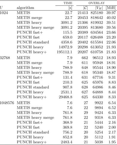
Partitioning. The performance of the overlay approach depends heavily on the number of boundary arcs of the underlying partition. Still, previous implementations of the overlay approach used out-of-box graph partitioning algorithms like METIS [44], SCOTCH [53], planar separators [46, 40], or grid partitions [43] for this step. Since these algorithms are not tailored to road networks, they output partitions of rather poor quality. More recently, Delling et al. [16] developed PUNCH, a graph partitioning algorithm that routinely finds solutions with half as many boundary arcs (or fewer) as the general-purpose petitioners do. The main reason for this superior quality is that PUNCH exploits the natural cuts that exist in road networks, such as rivers, mountains, and highways. It identifies these cuts by running various local maximum flow computations on the full graph, then contracts all arcs of the graph that do not participate in natural cuts.

The final partition is obtained by running heavy heuristics on this much smaller fragment graph. PUNCH outputs a high-quality partition with at mostU vertices per cell, whereU is an input parameter. Users can also specify additional parameters to determine how much effort (time) is spent in finding natural cuts and the heavy heuristics. In general, more time leads to better partitions, with fewer cut arcs. For further details, we refer the interested reader to the original work [16]. Moreover, note that, since the initial publication of PUNCH, great advances in general graph partitioning have been achieved. State-of-the-art partitioners like KaHiP [57], which use natural cut heuristics from PUNCH, generate partitions of quality similar to PUNCH.

We run PUNCH on the input graph with the following arc costs. Road segments open in both directions (most roads) have cost 2, while one-way road segments (such as freeways) get cost 1. We then use PUNCH to generate an L-level partition (with maximum cell sizes U1, . . . , UL) in top-down fashion. We first run PUNCH with parameterUL to obtain the top-level cells. Cells in lower levels are then obtained by running

PUNCH on individual cells of the level immediately above. To ensure similar running times for all levels, we set the PUNCH parameters so that it spends more effort on the topmost partition, and less on lower ones.

The exact parameters can be found in Section 7.

As our experiments will show, PUNCH is slower than popular general partitioners (such as METIS).

Since the metric-independent preprocessing is run very infrequently, however, its running time is not a major priority in our setting. Customization and query times, in contrast, should be as fast as possible, and (because we create cliques) their running times roughly depend on the square of the cut size. Still, PUNCH runs in tens of minutes on a standard server, which is fast enough to repartition the network frequently.

Moreover, one can handle a moderate number of new road segments by simply patching the original partition.

If both endpoints of a new arc are in the same bottom-level cell, no change is needed; if they are in different cells, we simply add a new cut arc. A full reoptimization is only needed when the quality of the partition decreases significantly.

To represent a multilevel partition within our algorithm, we use an approach similar to the one introduced for SHARC [10]. Each cell (at level 1 or higher) is assigned a unique sequential identifier within its supercell.

Since the number of levels and the number of cells per supercell are small, all identifiers for a vertex v can be packed in a single 64-bit integerpv(v), with the lower bits representing lower levels. For additional space savings, we actually storepvonly once for each cell on level 1, since it can be shared by all vertices in the cell. To determinepv(v), we first look up the cell v is assigned to on level 1, then access itspvvalue. This data structure requires 4·n+ 8· |C¹|bytes, including the 32-bit integer we store with each vertex to represent its level-1 cell.

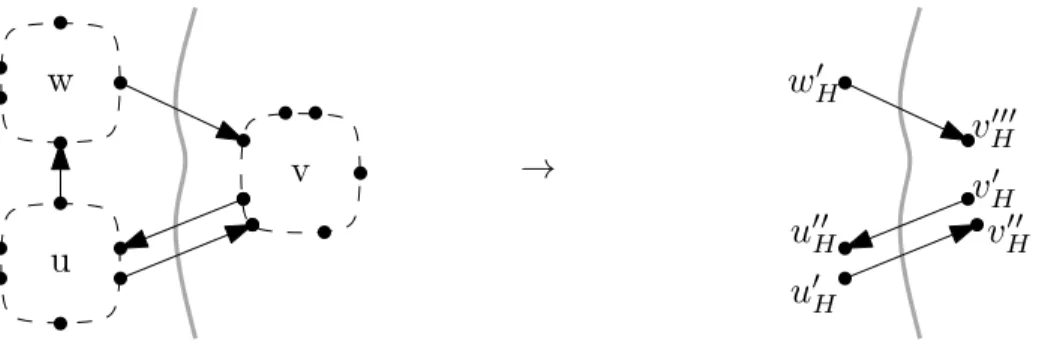
Overlay Topology. After partitioning the graph, we set up the metric-independent data structures of the overlay graph. The goal is to store the overlay topology only once, and allow it to be shared among all metrics. Regardless of the cost function used during customization and queries, we know the number of vertices and arcs of each overlay graph. For each boundary arc (u, v), we store two overlay vertices:u⁰_H, the appropriate exit point of intersectionu, andv_H⁰⁰, the appropriate entry point of intersectionv. We call u⁰_H anexit vertex of cellc1(u) andv_H⁰⁰ anentry vertex of cellc1(v). We also add an arc (u⁰_H, v_H⁰⁰) to the overlay, and store a pointer from this arc to the original arc inGto determine its cost when needed. Note that if the reverse arc (v, u) exists, we will add two additional vertices as well. See Figure 3 for an example. Also note that by introducing entry and exit vertices, we actually have a complete bipartite graph per cell (and not a clique).

Recall that we use nested partitions. Hence, a vertex (or cut arc) in any of the overlay graphs must be inH1as well. Therefore, we can store each overlay vertex only once with markers indicating whether it is a boundary vertex on each level. To improve locality, we assign IDs to overlay vertices such that the boundary vertices of the highest level have the lowest IDs, followed by the boundary vertices of the second highest level (which are not on the highest), and so on. Within a level, we keep the same relative ordering as in the original graph.

u

v w

→

u

u

v

v

w

v

Fig. 3.Building the overlay graph from the cut arcs. Each cut arc (u, v) yields two vertices u⁰_H,v⁰⁰_H in the overlay graph.

During queries, we must be able to switch efficiently (in both directions) between the original graph and the overlay. As Section 5.3 will explain, the switch can only happen at cut arcs. Therefore, for each vertex of the overlay graph, we explicitly store the corresponding vertex in the original graph, as well as which entry/exit point it refers to. For the other direction, we use a hash table to map triples containing the vertex (intersection), turn order, and point type (exit or entry) to vertices in the overlay. Recall that only boundary vertices must be in the hash table.

Moreover, to speed up the customization phase, for each vertex in G we also store a local identifier.

Within each level-1 cell, vertices have local identifiers that are unique and sequential (between 0 andU1−1).

For the same reason, each level-1 cell keeps the list of vertices it contains.

Finally, for each cell we must represent an overlay graph connecting its boundary vertices. Since our overlays are collections of complete bipartite graphs, we can represent them efficiently as matrices. A cell withpentry points andqexit points corresponds to ap×qmatrix in which position (i, j) contains the cost of the shortest path (within the cell) from the cell’si-th entry vertex to itsj-th exit vertex. We need one matrix for each cell in the overlay (on all levels). They can be compactly represented as a single (one-dimensional) arrayW: it suffices to interpret the matrix associated to each cellCas an array of lengthpCqC(in row-major order), then concatenate all arrays.

Note that the actual contents of W cannot be computed during the metric-independent preprocessing, since they depend on the cost function. In fact, each metric will have its own version ofW. But we still need auxiliary data structures to access and evaluate the matrices efficiently, however. Since they are shared by all metrics, they are set up during the metric-independent preprocessing stage.

First, for each cell C in the overlay graph, we keep three integers:pC (the number of entry points),qC

(the number of exit points), andfC (the position inW where the first entry ofC’s matrix is represented).

During customization and queries, the cost of the shortcut between the i-th entry point and the j-th exit point ofC will be stored inW[fC+iqC+j].

In addition, we maintain maps to translate (both ways) between a vertex identifier in the overlay graph and its position among the entry or exit vertices in the corresponding cells. More precisely, if an overlay vertex v is the i-th entry (or exit) point of its cell C at level l, we must be able to translate (v, l) into i, as well as (C, i) into v. Since identifiers are sequential and the number of levels is a small constant, simple arrays suffice for that.

Finally, to allow access to the cell number of an overlay vertex on each level, we also store the encoded level information pv for the overlay graph. This increases the memory overhead slightly (by 8 bytes per overlay vertex), but by avoiding expensive indirections it accelerates customization and queries.

Note that the vertices of the overlay graph do not have turn tables; the actual turn costs are encoded into the cost of the shortcut arcs, which we determine during the next phase.

5.2 Customization

The customization phase has access to the actual cost function that must be optimized during queries.

Because we have the metric-independent data structures in place, all we need to do is compute the entries of the above-mentioned arrayW, which represents the costs of all shortcuts between entry and exit vertices within cells.

We compute these distances in a bottom-up fashion, one cell at a time. Consider a cell C in H1 (the first overlay level). For each entry (overlay) vertex v in C, we run Dijkstra’s algorithm inG (restricted to C) until the priority queue is empty. This computes the distances to all reachable exit vertices ofC. Since we work on the underlying graph, we must use the turn-aware implementation of Dijkstra, as explained in Section 4.1.

A cellCat a higher levelHi (fori >1) can be processed similarly, with one major difference. Instead of working on the original graph, we can work on the subgraph ofH_i−1 (the overlay level immediately below) corresponding to subcells of C. This subgraph is much smaller than the corresponding subgraph of G. In addition, since overlay graphs have no (explicit) turns, we can just apply the standard version of Dijkstra’s algorithm, which tends to be faster.

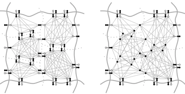
Fig. 4.The overlay graph before (left) and after (right) pruning.

Acceleration Techniques. Since customization is executed whenever a new metric must be optimized, we want this phase to be as fast as possible. We propose several optimizations that can speed up the basic algorithm describe above. We explain each optimization in turn, but they can be combined in the final algorithm.

Improving Locality. Conceptually, to process a cellC on level iwe could operate on the full overlay graph Hi−1, but restricting the searches to vertices insideC. For efficiency, we actually create a temporary copy of the relevant subgraph GC ofHi−1 in a separate memory location, run our searches on it, then copy the results to the appropriate locations inW. This simplifies the searches, allows us to use sequential local IDs, and improves locality. For the lowest level, instead of operating on the turn-aware graph, we extract an arc- based (see Section 4.1) subgraph. This allows us to use standard (non-turn-aware) graph search algorithms and other optimizations, which we discuss next.

Pruning the Search Graph. To process a cellCofHi, we must compute the distances between its entry and exit points. For a leveli >1, the graphGC on which we operate is the union of subcell overlays (complete bipartite graphs) with some boundary arcs between them (see Fig. 4). Instead of searching GC directly, we first contract its internal exit points. Since each such vertex has out-degree one (its outgoing arc is a boundary arc withinC), this reduces the number of vertices and arcs in the search graph. AlthoughC’s own exit points must be preserved (they are the targets of our searches), they do not need to be scanned (they have no outgoing arcs). We do not perform this optimization on the lowest level (H1), since the number of degree-one vertices is very small.

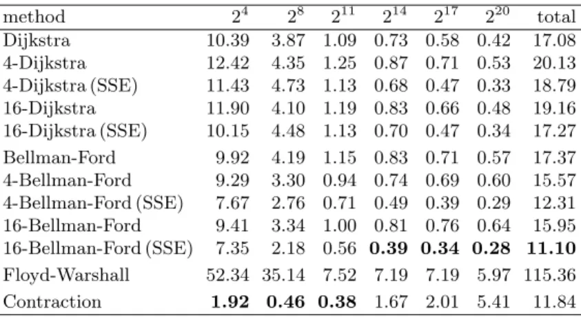
Alternative Algorithms. We can further accelerate customization by replacing Dijkstra’s algorithm with the well-known Bellman-Ford algorithm [12, 27]. It starts by setting the distance label of the source vertex to 0, and all others to∞. Each round then scans each vertex once, updating the distance label of its neighbors appropriately. For better performance, we only scan active vertices (i.e., those whose distance improved since the previous round) and stop when there is no active vertex left. While Bellman-Ford cannot scan fewer vertices than Dijkstra, its simplicity and better locality make it competitive for small graphs (such as the ones we operate on during customization). The number of rounds is bounded by the maximum number of arcs on any shortest path, which is small for reasonable metrics but linear in the worst case. One could therefore switch to Dijkstra’s algorithm whenever the number of Bellman-Ford rounds reaches a given (constant) threshold.

For completeness, we also tested the Floyd-Warshall algorithm [26]. It computes shortest paths among all vertices in the graph, and we just extract the relevant distances. Its running time is cubic, but with its tight inner loop and good locality, it could be competitive with Bellman-Ford on denser graphs.

Multiple-source executions. Multiple runs of Dijkstra’s algorithm (from different sources) can be accelerated if combined into a single execution [38, 64]. We apply this idea to the Bellman-Ford executions we perform within each cell. Let k be the number of simultaneous executions, from sourcess1, . . . , sk. For each vertex v, we keepk distance labels:d1(v), . . . , dk(v). All di(si) values are initialized to zero (each si is the source of its own search), and all remainingdi(·) values to∞. Allksourcessi are initially marked as active. When Bellman-Ford scans an arc (v, w), we try to update all k distance labels of w at once: for each i, we set di(w) ← min{di(w), di(v) +`(v, w)}. If any such distance label actually improves, we mark w as active.

This simultaneous execution needs as many rounds as the worst of the k sources, but, by storing the k distances associated with a vertex contiguously in memory, locality is much better. In addition, it enables instruction-level parallelism [64], as discussed next.

Parallelism. Modern CPUs have extended instruction sets with SIMD (single instruction, multiple data) operations, which work on several pieces of data at once. In particular, the SSE instructions available in x86 CPUs can manipulate special 128-bit registers, allowing basic operations (such as additions and comparisons) on four 32-bit words in parallel.

Consider the simultaneous execution of Bellman-Ford fromk= 4 sources, as above. When scanningv, we first storev’s four distance labels in one SSE register. To process an arc (v, w), we store four copies of`(v, w) into another register and use a single SSE instruction to add both registers. With an SSE comparison, we check if these tentative distances are smaller than the current distance labels forw(themselves loaded into an SSE register). If so, we take the minimum of both registers (in a single instruction) and markwas active.

Besides using SIMD instructions, we can use core-level parallelism by assigning cells to distinct cores. In addition, we parallelize the highest overlay levels (where there are few cells per core) by further splitting the sources in each cell into sets of similar size, and allocating them to separate cores (each accessing the entire cell).

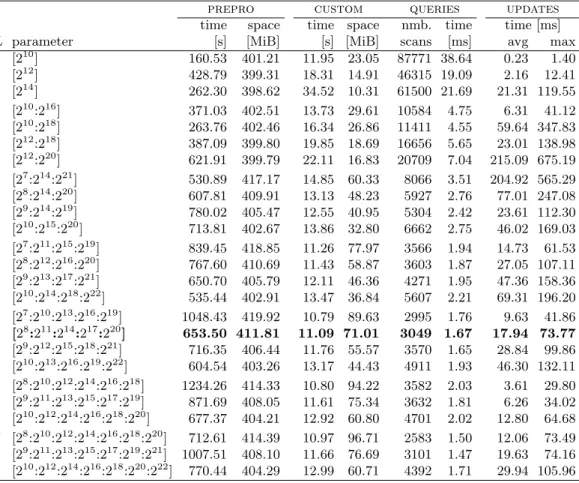
Phantom Levels. As our experiments will show, using more levels (up to a point) tends to lead to faster customization, since each level can operate on smaller graphs. Unfortunately, adding more levels also increases the metric-dependent space consumption. To avoid this downside, it often pays to introducephantom levels, which are additional partition levels that are used only to accelerate customization, but are not kept for queries. This keeps the metric-dependent space unaffected. Note, however, that we still need to build the metric-independent data structures for all levels, increasing the metric-independent space consumption during customization.

Incremental Updates. Today’s online map services receive a continuous stream of traffic information. If we are interested in the best route according to the current traffic situation, we need to update the overlay graphs. The obvious approach is to rerun the entire customization procedure as if we get a new metric. If only a few arcs (u0, v0), . . . ,(uk, vk) change their costs, however, we can do better. We first identify all cells cl(ui) andcl(vi) for all updated arcsiand all levels l. Only these cells areaffected by the update. Since we restrict searches during customization to the cells, we know that it is sufficient to rerun the customization only for these affected cells.

5.3 Query

Our query algorithm takes as input a source arcas, a target arcat, the original graphG, the overlay graph H =∪_iHi, and computes the shortest path between the head vertexsofas and the tail vertext ofat. We first explain a unidirectional algorithm that computes a path with shortcuts, then consider a bidirectional approach and explain how to translate shortcuts into the corresponding underlying arcs.

Basic Algorithm. Given any vertexv, define its query level lst(v) as the highest level such that v is not at the same cell assort. Equivalently,lst(v) is the maximumisuch thatci(v)∩ {s, t}=∅. As discussed by Holzer et al. [39], this is the level at whichv must be scanned if we find it during the search. The main idea is that one can skip cells that do not containsor t, and use shortcuts instead.

To computelst(v), we first determine the most significant differing bit of pv(s) andpv(v). (Recall that pv(v) encodes the cell number of v on each level.) This bit indicates the topmost levells(v) in which they differ. We do the same forpv(t) andpv(v) to determinelt(v). The minimum ofls(v) andlt(v) islst(v).

The query algorithm maintains a distance labeld(u) for each entryuwhich can either be a vertex on the overlay or a pair (v, i) corresponding to the i-th entry point ofv in the original graph. It also maintains the costµ of the shortest path seen so far; all variables are initialized to ∞. Since we always start a query on the original graph, we setd(s, i) = 0 and add the corresponding entry to the priority queue.

Each iteration of the algorithm takes the minimum-distance entry from the queue, representing either an overlay vertexuor a pair (u, i) from the original graph. If the entry is a pair, we scan it using the turn-aware version of Dijkstra’s algorithm (and look at its neighbors inG). Otherwise, we use the overlay graph at level lst(u), which does not have turns. In either case, the neighborsv ofuare added to the priority queue with the appropriate distance labels. Note that a level transition occurs whenuandvhave different query levels;

in particular, for transitions from or to level 0, we must translate between the two vertex identifiers forv (in Gand inH), which can be done in constant time using the metric-independent data structures described in Section 5.1.

As described in arc-to-arc queries with plain unidirectional Dijkstra (Section 4.2), we updateµwhenever we scan t, and the search terminates when it is about to scan a vertex whose distance label is greater than µ. We can retrieve the path with shortcuts by keeping a parent pointer for each vertex.

We apply several optimizations. First, by construction, each exit vertex u in the overlay has a single outgoing arc (u, v). Therefore, during the search we do not adduto the priority queue; instead, we traverse the arc (u, v) immediately and processv. This reduces the number of heap operations. We still store a distance value atu, though. A second optimization uses the fact that the maximum heap size can be computed in advance. Any search will scan at most all overlay vertices and the vertices in the cells ofsandton the lowest level. This allows us to preallocate all necessary data structures. To index the heap, we use local identifiers (for vertices in the source and target cells, with different offsets), and overlay identifiers otherwise. Finally, we keep track of all vertices touched by one quick, allowing for a quick initialization of the next one.

Bidirectional Search. We can accelerate queries even further by running bidirectional search. The forward search works as before, starting from the head vertex ofas and operating on entry points of vertices. The backward search is symmetric: it starts from the tail vertex of at and works on the reverse graph, which means it maintains distance labels forexit pointsinstead. Whenever we scan (during the forward or backward search) a vertexv that has been seen by the opposite direction, we update µ. Note that ifv ∈G, we have to evaluate all possible turns at v because the forward search operates on the entry points of v, and the backward search on the exit points. The search terminates as soon as the sum of the minimum keys of both priority queues (forward and backward) exceedsµ.

Note that, when processing the overlay graph, the backward search may access the matrices within each cell in a cache-inefficient way, since they are represented in row-major order. Keeping a second copy of each matrix (transposed) would only improve overall running times by about 15%, which is not enough to justify doubling the amount of metric-dependent data. We therefore opt to store each matrix only once.

Path Unpacking. Up to now, we have only discussed how to compute the distance between two arcs.

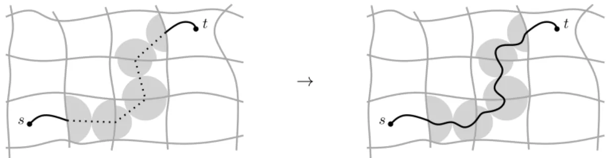
Following the parent pointers of the meeting vertex (the vertex that was responsible for the last update ofµ) of forward and backward searches, we obtain a path that potentially containing shortcuts. To obtain the complete path description as a sequence of arcs (or vertices) in the original graph, each shortcut in the result must be translated (unpacked) into the corresponding subpath. An obvious approach is to store this information for each shortcut explicitly, but this is wasteful in terms of space. Instead, we recursively unpack a level-ishortcut (v, w) by running bidirectional Dijkstra between v andwon leveli−1, restricted

s

t

→

s

t

Fig. 5.Shortcut unpacking. A shortcut on the shortest path is processed by running a local version of bidirectional Dijkstra on the level below (left). This results in a path consisting of arcs from the level below (right).

to subcells of the level-icell containing the shortcut. See Fig. 5 for an illustration. This does not increase the metric-dependent space consumption, and query times are still small enough. Note that disjoint cells can be handled in parallel.

If even faster unpacking times are needed, the customization phase could store a bit with each arc at leveli−1 indicating whether it appears in a shortcut at leveli. Only arcs with this bit set need to be visited during the unpacking process. This approach increases the metric-dependent amount of data stored only slightly, and does accelerate queries. Unfortunately, it complicates the customization step.

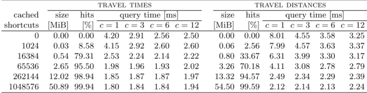
In practice, we use a simpler approach: we maintain a cache of frequently-used shortcuts. Each entry in the cache represents a level-i shortcut together with the corresponding sequence of level-(i−1) shortcuts.

Note that we have one cache with all shortcuts instead of having one cache for each level. As the experiments will show, with a standard least-recently used (LRU) update policy, even a small cache can accelerate path unpacking significantly.

Alternatives. In road networks, there often exist several routes fromstotwith similar overall costs. That is why a common feature for map service applications is to reportalternative routes besides the best route.

While the best route corresponds to the shortest path in the underlying graph, characterizing a “good”

alternative is less obvious. We follow the approach based on the concept ofadmissible paths [3]. Intuitively, an admissible path is significantly different from the shortest path, but it still “feels” reasonable and is not much longer. More precisely, given a shortest path Opt, they define a path P between s and t to be an (α, β, γ)-admissible alternative if it has the following properties:

1. Limited sharing.The sum of the costs of the arcs that appear in bothOpt andP is at mostγ·dist(s, t).

2. Local optimality. Every subpath ofP shorter thanα·dist(s, t) is a shortest path.

3. Bounded stretch.For each pair of vertices u, v∈P, it holds that`(Puv)≤(1 +)dist(u, v).

Finding such paths in general is hard, so Abraham et al. [3] restrict themselves tosingle via paths, defined as the concatenation of the shortest paths Opt_sv and Opt_vt for some vertex v (thevia vertex). They show that one can find such alternatives by running bidirectional query algorithms, such as bidirectional Dijkstra, contraction hierarchies (CH), or reach (RE). The main idea is to relax the stopping criterion so that many vertices are scanned by both searches (forward and backward). Each doubly-scanned vertexvis a candidate via vertex, and is evaluated according to the cost`(v) of the paths–v–t, how much that path shares with the shortest (indicated byσ(v)), and the so-calledplateau cost pl(v), which gives a bound on the local optimality of the path [13]. The plateau cost of a vertex v is defined by the cost of the subpath ofPv containing all verticesuwithdist(s, u) +dist(u, t) =`(v). To ensure no bad routes are reported to the user, they discard any vertex v that violates any of the admissibility constraints: `(v)< (1 +)·`(Opt), σ(v)< α·`(Opt), or pl(v) > γ·`(Opt). They then return as alternative the path Pv through the vertex v that minimizes the functionf(v) = 2`(v) +σ(v)−pl(v). As suggested by Abraham et al. [3], typical parameter values are α= 0.8, γ = 0.25, and = 0.3. Note that they return no alternative if all double-scanned vertices violate the admissibility constraints.

They also show that one can compute multiple alternatives by redefiningsharing to be the sum of costs of the arcs a path has in common withOpt and any previously selected alternative.

Adapting CRP to find single via paths is straightforward. We run the normal point-to-point query, but stop only when each search scans a vertex with distance label greater than (1 +)·µ. The candidate via vertices (those visited by both searches) are then be evaluated using the method described above. One advantage of using this approach with CRP instead of CH or RE is that we do not need to run additional point-to-point queries to reconstructPv. CH and RE need such queries because a vertex that is not part of the shortest path may have the wrong distance label, which is not the case for CRP.

Handling Traffic. One of the most important features of CRP is its fast customization, which enables (among other features) real-time traffic updates. As explained in Section 5.2, we can quickly update the overlay graphs whenever new traffic information is available. A standard query in the updated graph then will find the shortest path in traffic. When computing a very long journey, however, it may make sense to take the current traffic into account only when evaluating arcs that are sufficiently close to the source. After all, by the time the driver actually gets to faraway arcs, the traffic situation will most likely have changed. CRP can easily handle this scenario by keeping two cost functions, with and without the current traffic situation.

A modified (unidirectional) query algorithm then starts from sincorporating traffic and then switches to a non-traffic scenario after a certain time.

In practice, many traffic jams can be predicted from historic traffic information. Accordingly, the time- dependent route planning problem associates a travel time function to each arc in the graph, representing the time to traverse the road segment at a certain time of the day [21]. Dijkstra’s algorithm can still find the optimal solution in this scenario, as long as the functions are FIFO (i.e., no overtaking is allowed within an arc, which is a natural assumption in practice). CRP can therefore still be used, as long as we store time-dependent shortcuts. These are more costly to compute and take more space, but compression methods developed for time-dependent CH [7] should work here as well. Since historic traffic information is itself only an approximation (for future traffic), in practice one can allow small errors to improve efficiency and space consumption in the time-dependent scenario.

One can get the most accurate results by incorporating the current traffic situation at the beginning of the journey, then switching to a time-dependent scenario when far away froms.

5.4 Discussion

As already mentioned, CRP follows the basic strategy of separator-based methods. In particular, HiTi [43]

uses arc-based separators and cliques to represent each cell, just as we do. Unfortunately, HiTi has not been tested on large road networks; experiments were limited to small grids, and the original proof of concept does not appear to have been optimized using modern algorithm engineering techniques. The same holds for other implementations [40].

CRP improves on various aspects of previous implementations. First, by separating metric-independent from metric-dependent data, we can easily handle multiple metrics by changing a single pointer (to a different arrayW, representing the costs of the shortcuts). Second, we have carefully engineered every aspect of the algorithm to fit our target application. Finally, we have developed a partitioning algorithm that, by exploiting the natural cuts of road networks, finds significantly better partitions than previous approaches.

An important aspect of our work is to explore the design space comprehensively. For example, by forgoing known acceleration techniques such as arc reduction or sparsification (see Section 3.3), we were able to keep the topology of the overlay metric-independent, allowing it to be shared among all cost functions. Although using such techniques would make queries slightly faster (by less than a factor of 2), it would significantly slow down (and complicate) customization. Even worse, it would not allow the metric-independent data to be shared among cost functions.

Similarly, we decided not to use goal-directed speedup techniques such as ALT [35, 37], PCD [48], or Arc- Flags [45, 38] on the topmost overlay graph, despite the apparent advantages reported in previous work [41, 11]. We tested some of these techniques, and the impact on query performance was again limited (less

than a factor of 2), but its implementation became much more complicated. For example, queries now need to be executed in 2 phases [11], which requires a more complicated algorithm and makes local queries slower. Moreover, these techniques require metric-dependent preprocessed data, which significantly increases customization times. On balance, using goal-direction on the topmost level is not worth the effort.

We stress that CRP could be further optimized to handle a large number of (perhaps personalized) cost functions. Most likely, a particular cell will have the exact same cost matrix (overlay) for multiple cost functions. (For example, a metric such as “avoid tolls” could only differ from the standard metric in cells containing toll booths.) We could avoid duplication (and save space) by maintaining a pool of unique matrices, and making each cost function keep pointers to the relevant cells in the pool.

6 Accelerating Customization by Contraction

As our experiments will show, separating preprocessing from metric customization allows CRP to incorporate a new cost function on a continental road network in about 10 seconds (sequentially) on a modern server. This is enough for real-time traffic, but still too slow to enable on-line personalized cost functions. Accelerating customization even further requires speeding up its basic operation: computing the costs of the shortcuts within each cell.

In the Section 5.2, we already discussed several optimization techniques for computing shortcut costs. In this section, we discuss how we can use contraction, the basic building block of the contraction hierarchies (CH) algorithm [32], to accelerate the customization phase even further. Instead of computing shortest paths explicitly, we eliminate internal vertices from a cell one by one, adding new arcs as needed to preserve distances; the arcs that eventually remain are the desired shortcuts. For efficiency, not only do we precompute the order in which vertices are contracted, but also abstract away the graph itself. During customization, we simply simulate the actual contraction by following a (precomputed) series ofinstructions describing the basic operations (memory reads and writes) the contraction routine would perform.

Thecontractionapproach is based on theshortcutoperation [56, 32]. To shortcut a vertexv, one removes it from the graph and adds new arcs as needed to preserve shortest paths. For each incoming arc (u, v) and outgoing arc (v, w), one creates ashortcutarc (u, w) with`(u, w) =`(u, v)+`(v, w). A shortcut is only added if it represents the only shortest path between its endpoints in the remaining graph (withoutv), which can be tested by running awitness search (local Dijkstra) between its endpoints. CH uses contraction as follows.

During preprocessing, it heuristically sorts all vertices in increasing order of importance and shortcuts them in this order; the order and the shortcuts are then used to speed up queries.

We propose using contraction during customization. To process a cell, we can simply contract its internal vertices while preserving its boundary vertices. The arcs (shortcuts) in the final graph are exactly the ones we want. If we want to compute multiple overlay levels with contraction, we also need to remember which intermediate shortcuts contribute to W. To deal with turn costs appropriately, we run contraction on the arc-based graph.

The performance of contraction strongly depends on the cost function. With travel times in free-flow traffic (the most common case), it works very well. Even for continental instances, sparsity is preserved during the contraction process [32], and the number of arcs less than doubles. Unfortunately, other metrics often need more shortcuts, which leads to denser graphs and makes finding the contraction order much more expensive. Even if a good order is given, simply performing the contraction can still be quite costly [32].

Within the CRP framework, we can deal with these issues by exploiting the separation between metric- independent preprocessing and customization. During preprocessing, we compute a unique contraction order to be used by all metrics. Unlike previous approaches [32], to ensure this order works well even in the worst case, we simply assume that every potential shortcut will be added. Accordingly, we do not perform witness searches during customization. Moreover, for maximum efficiency, we precompute a sequence of microinstructions to describe the entire contraction process in terms of basic operations. We detail each of these improvements next.