Ocean Drilling
Ruediger Stein1,2
1Alfred Wegener Institute Helmholtz Centre for Polar and Marine Research, Bremerhaven, Germany,2MARUM and Faculty of Geosciences, University of Bremen, Bremen, Germany
Abstract
Over the past 3–4 decades, coincident with global warming and atmospheric CO2increase, Arctic sea ice has significantly decreased in its extent as well as in thickness. When extrapolating this alarming trend, the central Arctic Ocean might become ice‐free during summers within about the next 2–5 decades. Paleoclimate records allow us to better understand the processes controlling modern climate change and distinguish between natural and anthropogenic forcing. In this context, detailed studies of the earlier Earth history characterized by a much warmer global climate with elevated atmospheric CO2concentrations are important. The main focus of this review paper is the long‐term late Mesozoic‐Cenozoic Arctic Ocean climate history from Greenhouse to Icehouse conditions, with special emphasis on Arctic sea ice history. Starting with some information on the Cretaceous Arctic Ocean climate, this paper will concentrate on selected results from Integrated Ocean Drilling Program (IODP) Expedition 302 (Arctic Ocean Coring Expedition (ACEX)), thefirst scientific drilling in the permanently ice‐covered Arctic Ocean, dealing with the Cenozoic climate history. While these results from ACEX were unprecedented, key questions related to the Cenozoic Arctic climate history remain unanswered, largely due to the major mid‐Cenozoic hiatus (if existing) and partly to the poor recovery of the ACEX record. Following‐up ACEX and its cutting‐edge science, a second scientific drilling on Lomonosov Ridge with a focus on the
reconstruction of the continuous and complete Cenozoic Arctic Ocean climate history has currently been proposed and scheduled as IODP Expedition 377 for 2021.
1. Introduction
During the last few decades, the remote Arctic Ocean, characterized by strong seasonal forcing and variabil- ity in runoff, sea ice formation, and sunlight, became a major focus within the ongoing debate of climate change as the high latitudes mirror the global warming trend strongly amplified (AMAP, 2017; Park et al., 2018; Serreze & Barry, 2011; Stocker et al., 2013). Due to complex feedback processes (collectively known as“polar amplification”), the Arctic is both a contributor of climate change and a region that will be most affected by global warming (ACIA, 2004, 2005; Serreze & Barry, 2011; Stocker et al., 2013). That means, the Arctic Ocean and surrounding areas are (in real time) and were (over historic and geologic timescales) subject to rapid and dramatic change. Although the Arctic Ocean was and is a key player in the past, present, and future global climate/Earth system (AMAP, 2017; Stocker et al., 2013), the marine geoscience research in the Arctic lags behind other world oceans, especially from a paleoclimatic perspective (e.g., Jakobsson et al., 2014; Stein, 2008). That means, detailed records of the short‐and long‐term geological and paleocli- mate history of the Arctic Ocean are still sparse. This lack in knowledge is mainly due to the major technological/logistical problems in operating within the permanently ice‐covered Arctic region.
During the last ~20 years, several international expeditions have greatly advanced our knowledge on central Arctic Ocean paleoenvironment and its variability through Quaternary times (Stein et al., 2015). Prior to 2004, however, central Arctic Ocean piston and gravity coring was mainly restricted to obtaining near‐
surface sediments; that is, only the upper 15 m could be sampled. Thus, almost all studies were restricted to the late Pliocene/Quaternary time interval, with only a few exceptions based on short sediment cores representing some isolated sections of late Mesozoic/early Cenozoic climate history. A breakthrough in Arctic Ocean paleoclimate research was thefirst scientific drilling in the permanently ice‐covered central Arctic Ocean that was carried out within the Integrated Ocean Drilling Program (IODP) in 2004, that is,
©2019. American Geophysical Union.
All Rights Reserved.
Key Points:
• Arctic climate records from Cretaceous‐Paleogene Greenhouse to Neogene‐Quaternary Icehouse help to understand modern climate change
• Ice‐free summers occurred during a late Miocene warm climate with pCO2 concentrations of 450 ppm, a value we might reach in the near future
• An IODP drilling on Lomonosov Ridge with a focus on the complete Cenozoic Arctic Ocean climate history is scheduled for 2021
Correspondence to:
R. Stein,
ruediger.stein@awi.de
Citation:
Stein, R. (2019). The late Mesozoic‐Cenozoic Arctic Ocean climate and sea ice history: A challenge for past and future scientific ocean drilling.Paleoceanography and Paleoclimatology,34. https://doi.org/
10.1029/2018PA003433
Received 20 JUN 2019 Accepted 27 AUG 2019
Accepted article online 6 NOV 2019
IODP Expedition 302—the Arctic Ocean Coring Expedition (ACEX), penetrating 428 m of Upper Cretaceous to Quaternary sediments on the crest of Lomonosov Ridge between 87° and 88°N (Backman et al., 2006;
Moran et al., 2006). The main objectives of the ACEX drilling campaign focused on the reconstruction of Cenozoic Arctic ice, temperatures, and climates from early (Paleogene) Greenhouse to modern‐type (Neogene) Icehouse conditions. Some of the key questions to be answered from ACEX were framed around the evolution of sea ice and ice sheets, the past physical oceanographic structure, Arctic gateways, links between Arctic land and ocean climate, and major changes in depositional environments (Backman et al., 2006, Backman et al., 2008; Backman & Moran, 2009; for reviews, see O'Regan et al., 2011; Stein, Blackman, et al., 2014; Stein, 2017). By studying the unique ACEX sedimentary sequence, >100 papers are now published in highly ranked international peer‐reviewed scientific journals (see Stein, Weller, et al., 2014, Stein et al., 2015, for references). Some of the ACEX paleoceanographic themes and highlights with reference to the original literature are summarized in some more detail (see section 5.2). To date, the ACEX site remains the one and only scientific drilling location in the central Arctic Ocean (Figure 1).
Thus, thinking about scientific ocean drilling campaigns that have been carried out under the umbrella of the Deep‐Sea Drilling Project (DSDP), the Ocean Drilling Program (ODP), and/or the Integrated Ocean Drilling Program/International Ocean Discovery Program (IODP) in the other world oceans during the lastfive decades (Stein, Blackman, et al., 2014; Koppers et al., 2019), the Arctic Ocean is still a“mare incognitum”(Figure 1).
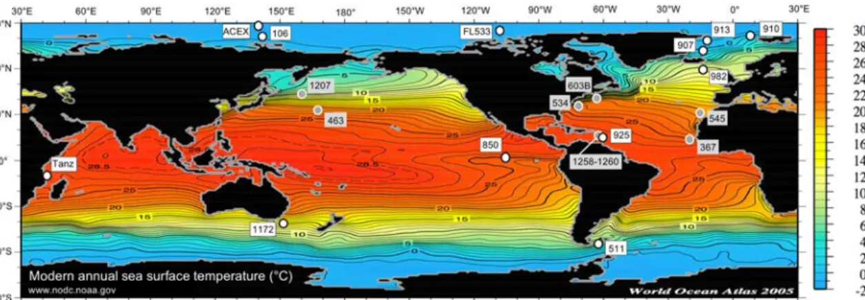
This review paper is structured as follows: After an overview about the main characteristics, significance, and recent climate change of the Arctic Ocean (sections 2 and 3) and some basic information about proxies used for the paleoenvironmental reconstructions (section 4), the main focus is on the long‐term late Figure 1.Arctic Ocean drilling: Emergingfields and new topics in an unknown area“mare incognitum.”Google map showing the Northern Hemisphere with locations of Deep‐Sea Drilling Project, ODP, and IODP sites; selected high northern latitude expeditions are highlighted. Locations of ODP sites 907, 910, 913, and 982 for which SST records are included in Figure 15 are shown as well. Large white circles indicate the connection via Fram Strait between Greenland and Svalbard, and Bering Strait between Alaska and Siberia to the Atlantic Ocean and Pacific Ocean, respectively. White arrows indicate discharge into the Arctic Ocean by major rivers. BS = Beaufort Sea, BeS = Bering Sea, CS = Chukchi Sea, ESS = East Siberian Sea, LS = Laptev Sea, KS = Kara Sea, BaS = Barents Sea. The location of the ACEX drill site and the working area of the IODP Expedition 377 (ArcOP) are shown in red.
Mesozoic‐Cenozoic climate history from Greenhouse to Icehouse conditions, with special emphasis on the Arctic sea ice history during its course from ice‐free to seasonal to permanent ice conditions (section 5).
Starting with some information on the Cretaceous climate based on short gravity cores, this paper will concentrate on selected results from IODP Expedition 302 (ACEX) dealing with the Cenozoic climate history. Finally, an outlook on the key goals of the coming IODP Expedition 377 scheduled for 2021 will be presented (section 6).
2. The Arctic Ocean: Characteristics and Significance for the Climate System
What are the main characteristics that make the Arctic Ocean so unique in comparison to the other world oceans? Why is the Arctic Ocean so important in the global climate/Earth system? Several aspects can be listed:
2.1. Physiography and Water Mass Exchange
The Arctic Ocean is surrounded by continents and the world's largest shelf seas, with limited connections to the Pacific and Atlantic Oceans, making the Arctic Ocean a“Mediterranean Sea”(Figure 1). With an area of about 9.5 × 10⁶km2, the entire Arctic Ocean comprises 2.6% of the total area of the world's oceans, but less than 1% of the volume (about 13 × 106km3; Jakobsson, 2002; Jakobsson et al., 2012). The relatively small total volume is due to the large shelf areas, which make up as much as 52.7% of the total area of the Arctic Ocean, resulting in a shallow mean depth of the entire Arctic ocean of about 1,360 m.
Fram Strait between northeastern Greenland and Svalbard is the only deep‐water connection with the world ocean via the Atlantic Ocean (Figures.1 and 2). Furthermore, two major currents, with southwardflowing waters on the west and northwardflowing waters on the east, exchange surface‐water water between the Arctic and the North Atlantic through Fram Strait (Figure 3; Aagaard et al., 1985; Rudels et al., 1994;
Schauer et al., 2002): The cold, ice‐transporting East Greenland Current is the main current out of the Arctic Ocean. In contrast, the eastern West Spitsbergen Current, an extension of the North Atlantic‐ Norwegian Current, carries warm, relatively saline Atlantic Water into the Arctic Ocean. This Atlantic Water branch cools down and, together with Atlantic water that isflowing across the Barents Sea and through the St. Anna Trough, follows the continental slope and ridges of the deep basins at intermediate water depths. Toward the Pacific Ocean, only a shallow‐water connection exists. From there, relative low‐ saline, nutrient‐rich Pacific Water enters the Arctic Ocean through the Bering Strait (Figure 2), primarily dri- ven by a pressure‐head difference between the Pacific and the Arctic Oceans (e.g., Coachman et al., 1975;
Hunt et al., 2012; Woodgate et al., 2005).
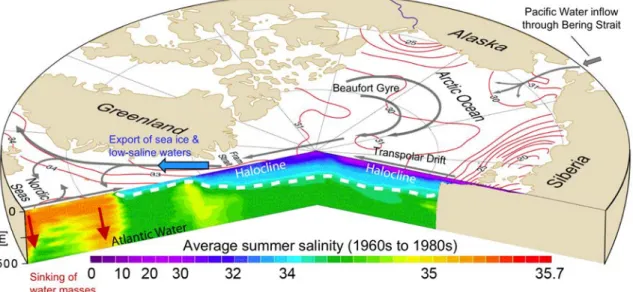
Figure 2.Map and vertical structure (500 m) of salinity in the Arctic Ocean. Inflow of Pacific Waters through Bering Strait and export of ice and low‐saline waters through Fram Strait are indicated. Gray arrows mark the average surface water circulation within the Beaufort Gyre and the Transpolar Drift and red arrows the places of sinking water masses (Spielhagen & Bauch, 2015, supplemented; based on data from EWG, 1998).
2.2. Surface‐Water Characteristics: Temperature and Salinity
Whereas the central Arctic Ocean mean sea‐surface temperatures (SST) are <−1 °C throughout the year (resulting in a permanent sea‐ice cover), a distinct seasonal variability is obvious in the marginal seas (Environmental Working Group, 1998; Singh et al., 2013). In the latter, mean SST reaches values of 0 to 5 °C during summer at times of increased river discharge and Atlantic Water inflow. During winter times, low mean SST of <−1 °C similar to those of the central Arctic Ocean were also measured in the marginal seas. An exception from this general picture is the Barents Sea, strongly influenced by Atlantic Water inflow.
Here mean summer SST may increase to 8 °C and even during winter time; values of up to 4 °C were deter- mined in the southwestern part.
The distribution of the sea‐surface salinity (SSS) is strongly controlled by the river discharge and the Atlantic Water inflow (Figure 2; Environmental Working Group, 1998). The high river discharge results in a very low salinity in the Arctic Ocean proper as well as the marginal seas, except for the Barents Sea, influenced by more saline Atlantic Water inflow. The Beaufort, East Siberian, Laptev, and Kara seas are characterized by mean SSS of <29 during the summer, strongly decreasing toward the river mouths; in most part of the central Arctic, mean SSS is below 32. In the Barents Sea and adjacent continental slope, mean SSS Figure 3.The extent of Arctic sea ice in 2017, showing the seasonal variability with maximum in March and minimum in September. During recent years, the sea ice extent has reduced significantly compared to the long‐term median of the years 1981 to 2010 shown as yellow line (Spreen et al., 2008; https://seaice.uni‐bremen.
de/arctic‐sea‐ice‐minima/). Beaufort Gyre (BG) and the Transpolar Drift (TPD) systems are shown as black arrows. Red arrows mark inflow of warm Atlantic waters, and blue arrow marks outflow of cold Arctic waters. WSC = West Spitsbergen Current, EGC = East Greenland Current. The location of the ACEX drill site and the working area of the IODP Expedition 377 (ArcOP) are shown in green.
increases to >34. Due to seasonal variability in river discharge, the SSS also displays a strong variability, especially in the marginal seas.
2.3. Sea‐Ice Cover
A key phenomenon of the Arctic Ocean is the perennial sea‐ice cover in its central part and a strong seasonal variation of sea ice in the surrounding marginal (shelf) areas (Figure 3; Johannessen et al., 2004; Thomas &
Diekmann, 2010; https://nsidc.org/data/seaice_index/). In winter these areas are usually completely cov- ered with ice, whereas in summer they are mostly ice‐free. An exception is the Barents Sea and the area around Svalbard, strongly influenced by the warm Norwegian/West Spitsbergen Current system. There, large parts are ice‐free throughout the year.
In general, there are two primary forms of sea ice: seasonal (orfirst‐year) ice and perennial (or multi‐year) ice.
The thickness offirst‐year ice ranges from a few tenths of a meter near the southern margin of the marine cryosphere to 2.5 m in the high Arctic at the end of winter. Somefirst‐year ice survives the summer and becomes multiyear ice. In the present climate, old multiyear icefloes without ridges are about 3 m thick at the end of winter. In addition, land‐fast ice (or fast ice) occurs in the coastal circum‐Arctic area, which is immobilized for up to 10 months each year by coastal geometry or by grounded ice ridges (ACIA, 2004, 2005).
Sea‐ice concentration (percent ice area per unit area) and derived parameters such as ice extent (the area within the ice‐ocean margin defined as 15% ice concentration) can be reliably retrieved through satellite‐ borne passive microwave sensors, which are available continuously since 1978 and operating independently of cloud cover and light conditions (Gloersen et al., 1992; Johannessen et al., 2004). Satellite data have shown that the area of sea ice decreases from roughly 14–15 ×106km2in March to <5–7 ×10⁶km2in September, as much of thefirst‐year ice melts during the summer (Figure 3; Gloersen et al., 1992; Cavalieri et al., 1997;
Johannessen et al., 2004; Stroeve et al., 2012; https://nsidc.org/). The area of multiyear sea ice, mostly over the Arctic Ocean basins, the East Siberian Sea, and the Canadian polar shelf, is about 4–5 ×10⁶km2having decreased significantly during the last decades (e.g., AMAP, 2017; Johannessen et al., 1999; Nghiem et al., 2007).
The mean sea‐ice drift pattern, a direct response to surface atmospheric pressure gradients and resulting wind patterns, is quite well known from drift buoy and geostrophic windfield data (Colony & Thorndike, 1985; Hibler, 1989; Pfirman et al., 1997; Thorndike & Colony, 1982). North of the Alaskan coast, the ice cir- culates in a big anticyclonic structure, the Beaufort Gyre (Figure 3), corresponding to the high‐pressure sys- tem over the Beaufort Sea. Speed varies from almost 0 in the center to 3 cm/s in the marginal zones. Toward the Siberian Arctic, this gyre opens up to a linear structure, the Transpolar Drift (Figure 3). Its origin is in the area of the Chukchi‐East Siberian Sea, and it leads to the West. Ice drifts with mean velocities of about 2 cm/s past the North Pole and Franz Josef Land, accelerating to mean values of up to 10 cm/s through Fram Strait between Svalbard and Greenland.
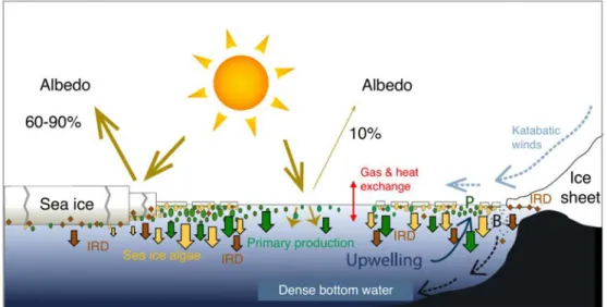
Sea ice is a very critical component of the Arctic system that responds sensitively to changes in atmospheric circulation, incoming radiation, atmospheric and oceanic heatfluxes, and the hydrological cycle (Figure 4).
Ice significantly reduces the heat flux between ocean and atmosphere; through its high albedo, it has a strong influence on the radiation budget of the entire Arctic. The albedo of open water is as low as 0.10, whereas the ice albedo ranges between 0.6 and 0.8 (Figure 4; Barry, 1996; Serreze & Barry, 2011). Thus, over ice surfaces as compared with open water, up to 8 times as much of the incoming shortwave radiation is reflected, resulting in lower surface temperatures. Furthermore, the sea‐ice cover strongly affects the biolo- gical productivity (e.g., Sakshaug, 2004), as a more closed sea‐ice cover restricts primary production due to low light influx into the surface waters (Figure 4). Sea ice is also an important agent for sediment transport from the shelves into, across, and out of the Arctic Ocean. Increased export of sea ice via the East Greenland Current will reduce the surface salinity in the Greenland Sea, which subsequently diminishes the global thermohaline circulation by slowing the production of North Atlantic Deep Water (Aagaard & Carmack, 1989; Broecker, 1997; Raymo et al., 1990).
2.4. River Discharge
One of the main characteristics of the Arctic Ocean is its huge river discharge (e.g., Aagaard & Carmack, 1989; Holmes et al., 2002, 2018). Today, the annual direct freshwater inflow by major rivers into the Arctic Ocean reaches a total of about 3,300 km3(Holmes et al., 2002, 2018; Rachold et al., 2004). For
comparison, the amount of water discharged by the world rivers to the present‐day ocean is estimated to be between 32 and 37 × 103km3/year (Milliman & Meade, 1983; Chakrapani, 2005). That means, the Arctic Ocean discharge is equivalent to >10% of the global runoff. Major contributors are the Yenisei (620 km3/ year), the Ob (429 km3/year), the Lena (525 km3/year), and the MacKenzie (249 km3/year; Figure 1;
Holmes et al., 2002, 2018; Rachold et al., 2004; McClelland et al., 2012).
The overall importance of Arctic river discharge for the Arctic Ocean and its significance for the global ocean system can be summarized as follows:
• Thefluvial fresh‐water supply is essential for the maintenance of the approx. 200‐m‐thick low‐salinity layer of the central Arctic Ocean and, thus, contributes significantly to the strong stratification of the near‐surface water masses (Figure 2), encouraging sea‐ice formation. Thus, changes in the fresh‐water balance would influence the extent of sea‐ice cover.
• The fresh‐water exported from the Arctic Ocean through Fram Strait influences global thermohaline cir- culation (Figure 2). Today, the annual liquid fresh‐water export of the East Greenland Current is about 1,160 km3. Estimates based on sea‐ice export even reach values of 1,680 (Aagaard & Carmack, 1989) to 2,850 km3/year (Eicken, 2004). Because factors such as the global thermohaline circulation as well as sea‐ice cover and earth albedo have a strong influence on the Earth's climate system, the fresh‐water input to the Arctic and its change through time may have triggered global climate changes in the past (e.g., the initiation of the Northern Hemisphere Glaciation during mid‐Pliocene times; Driscoll & Haug, 1998; for further discussion, see section 6).
• The Arctic rivers transport large amounts of nutrients, dissolved and particulate material (i.e., chemical elements, siliciclastic suspension, terrestrial organic matter, etc.; Martin et al., 1993; Gordeev et al., 1996; Stein & Macdonald, 2004; Bring et al., 2016), and anthropogenic pollutants (i.e., radioactive ele- ments, heavy metals, etc.; Nies et al., 1998; Crane et al., 2001) onto the shelves (see above) where it is accu- mulated or further transported by different mechanisms (sea ice, icebergs, turbidity currents, etc.) toward the open ocean (e.g., Stein, 2008 for review). Thus, river‐derived materials contribute in major proportions to the entire Arctic Ocean sedimentary and chemical budgets.
Figure 4.Simplified scheme of the role of sea ice in the climate and ocean system, indicating the modern central and ice‐ edge Arctic area (left) and the glacial Arctic situation with ice sheets reaching the shelf break, a situation similar to the modern circum‐Antarctic situation (right). Furthermore, solar energy (yellow‐olive arrows), katabatic winds (light blue arrow), albedo effect, and ocean processes such as upwelling and brine (B) formation, polynyas (P), phytoplankton production (little green circles), and sea‐ice algae (and IP25) production (little yellow circles) with relatedfluxes (green and yellow arrows, respectively) are shown. Figure adapted from De Vernal, Gersonde, et al. (2013), supplemented.
2.5. Permafrost
Large areas around the Arctic Ocean reaching about one quarter of the landmass of the Northern Hemisphere (Brown et al., 1997) are occupied by permafrost, that is, perennially frozen ground (Romanovskii et al., 2004; Vonk et al., 2015). The thickness of permafrost ranges from very thin layers of only a few centimeters thick to several hundreds of meters; in unglaciated areas of Siberia, even thicknesses of about 1,500 m may be reached (Washburn, 1980; Nelson et al., 1999). Furthermore, thermal modelling and geophysical data (e.g., Rekant et al., 2005; Romanovskii et al., 2005) indicate that large areas of the Arctic shelves, as a result of their exposure during the Last Glacial Maximum, are thought to be almost entirely underlain by subsea permafrost from the coastline down to a water depth of about 100 m (Rachold et al., 2007).
Many of the potential environmental and socioeconomic impacts of global warming in the Arctic are asso- ciated with permafrost. The effects of climatic warming on permafrost and the overlying“active layer“can severely disrupt ecosystems and human infrastructure and may intensify global warming (e.g., Frey et al., 2007; Jorgenson et al., 2001; Nelson et al., 1999). Huge amounts of soil organic carbon are currently stored frozen in permafrost soils (e.g., Tarnocai et al., 2009; Zimov et al., 2009), and vast amounts of methane, in a solid form as gas hydrates, are trapped in permafrost and at shallow depths in cold ocean sediments (e.g., Romanovskii et al., 2005). With increasing temperature of the permafrost (Romanovsky et al., 2010) and the water at the seafloor, as a result of increased surface warming in Arctic regions (Stocker et al., 2013), a widespread increase in the thickness of the thawed layer and the decomposition of hydrates could lead to the release of large quantities of CH4(and CO2) to the atmosphere (ACIA, 2004, 2005; Anisimov et al., 1997; Goulden et al., 1998; Michaelson et al., 1996) as well as an enhanced mobilization and export of old, previously frozen soil‐derived organic carbon (e.g., Bröder et al., 2018; Bröder et al., 2019; Schuur et al., 2008; Tesi et al., 2016; Vonk et al., 2012; Winterfeld et al., 2015, 2018). The release of these greenhouse gases in turn would create a positive feedback mechanism that can amplify regional and global warming.
3. Recent Arctic Climate Change, Future Predictions, and Paleorecords
During the 1990s, it became widely recognized that the Arctic was undergoing a dramatic change (Dickson et al., 2000; Macdonald, 1996; Morison et al., 2000; Moritz et al., 2002; Serreze et al., 2000). Over the past dec- ades, a significant increase in Siberian river discharge, associated with a warmer climate and enhanced pre- cipitation in the river basins, has been observed (Semiletov et al., 2000; Serreze et al., 2000; Peterson et al., 2002). At the same time, an increase in the amount and temperature of Atlantic Water inflow into the Arctic, a reduced sea‐ice cover, a thawing of permafrost, and a retreat of small Arctic glaciers are observed (Dickson et al., 2000; Serreze et al., 2000).
The most obvious indicator for the ongoing rapid changes in the climate state of our planet, however, is cer- tainly the observed loss in Arctic sea ice (Serreze et al., 2007; Notz & Stroeve, 2018; Stroeve & Notz, 2018).
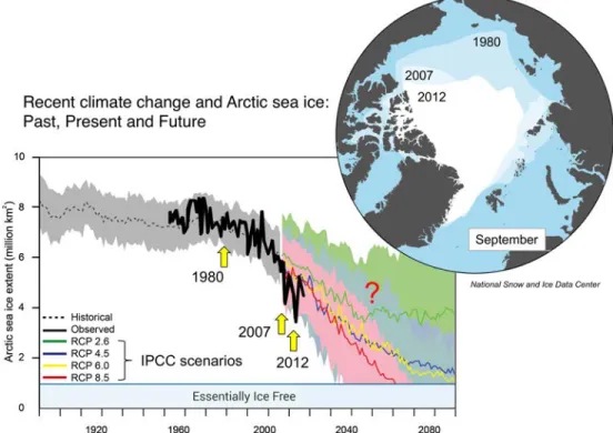
Over the past three to four decades, coincident with global warming and atmospheric CO2 increase, Arctic sea ice has significantly decreased in its extent (Figure 5) as well as in thickness (Cavalieri &
Parkinson, 2012; Kwok & Cunningham, 2015; Stocker et al., 2013; Stroeve et al., 2007, 2012). The loss of sea ice results in a distinct decrease in albedo, causing further warming of ocean surface waters. When extra- polating this trend, the central Arctic Ocean might become ice‐free during summers within about the next three to five decades or even sooner, depending on the different IPCC scenarios used for prediction (Figure 5; Wang & Overland, 2012; Stocker et al., 2013; Niederdrenk & Notz, 2018; Notz & Stroeve, 2018;
Stroeve & Notz, 2018; Screen & Deser, 2019). Furthermore, the recent decrease in sea ice seems to be more rapid than predicted by climate models (Figure 5; Stroeve et al., 2007, 2012), suggesting that the processes causing these recent rapid climate changes are still not fully understood and subject of intense scientific and societal debate. Based on the relationship between the September sea‐ice extent and cumulative atmo- spheric CO2emissions, however, Notz and Stroeve (2016) have demonstrated quite clearly that the observed decrease in sea‐ice cover is mainly driven by anthropogenic warming. Based on their records, these authors emphasized the importance of limiting future CO2emissions to values compatible with a global warming well below 2 °C in order to keep the ice cover during summer (cf.Sigmond et al., 2018 ; Stroeve & Notz, 2018). In any case, a key aspect within the debate about present climate change is to distinguish and quantify
more precisely natural and anthropogenic forcing of global climate change and related sea ice decrease (AMAP, 2017; Stocker et al., 2013).
In order to better understand the processes controlling modern climate change and distinguish between nat- ural and anthropogenic forcing, it is certainly very useful and important to study paleoclimate records. In general, such paleoclimate records document the natural climate, rates of change, and variability prior to anthropogenic influence. The instrumental records of temperature, salinity, precipitation, and other envir- onmental observations span only a very short interval (<150 years) of the Earth's climate history and provide an inadequate perspective of natural climate variability, as they are biased by an unknown amplitude of anthropogenic forcing. Paleoclimate reconstructions, however, can be used to assess the sensitivity of the Earth's climate system to changes of different forcing parameters (e.g., CO2) and to test the reliability of cli- mate models by evaluating their simulations for conditions very different from the modern climate. In this context, not only high‐resolution studies of the most recent (Holocene) climate history are of importance but also detailed studies of the earlier Earth history characterized by a much warmer (Greenhouse‐type) global climate with elevated atmospheric CO2concentrations, such as the Late Cretaceous and the Paleogene (Hong & Lee, 2012; Kent & Muttoni, 2013; O'Brien et al., 2017; Zachos et al., 2008). A precise knowledge of rates and scales of past climate change are the only mode to separate natural and anthropogenic forcings and will enable us to further increase the reliability of climate change predictions. Thus, understanding the mechanisms of natural climate change is one of the major challenges for mankind in the coming years. In this context, the polar regions certainly play a key role, and detailed climate records from the Arctic Ocean spanning time intervals from the Cretaceous‐Paleogene Greenhouse world to the Neogene‐ Quaternary Icehouse world will give new insight into the functioning of the Arctic Ocean within the global climate system.
Figure 5.September sea ice extent in the Arctic Ocean (1890–2090) based on historical data, direct observations/measure- ments, and projected by different climate models and different IPCC scenarios toward 2090. RCP = Representative Concentration Pathways of greenhouse gases in relation to the probable radiative forcing in 2100. The shaded area represents the standard deviation (Stocker et al., 2013; Stroeve et al., 2007; Stroeve et al., 2012). Map shows September sea‐ ice extent in 1980, 2007, and 2012 (Source: National Snow and Ice Data Center; https://nsidc.org/).
4. Proxies for Reconstructing Past Arctic Ocean Paleoenvironmental Conditions
What type of proxies are available for reconstruction of Arctic paleoclimate and, especially, paleo‐sea ice con- ditions? A large number of studies are based on sedimentological, mineralogical, geochemical, and geophy- sical data (e.g., Darby, 2003, 2008, 2014; Jakobsson et al., 2014; Knies et al., 2000; Nørgaard‐Pedersen et al., 2003; Polyak et al., 2010; Spielhagen et al., 2004), as well as microfossils such as diatoms, dinoflagellates, ostracods, coccoliths, and foraminifers (e.g., Koç et al., 1993; Matthiessen et al., 2001, Matthiessen, Brinkhuis, et al., 2009; Sarnthein et al., 2003; Polyak et al., 2010; de Vernal & Rochon, 2011; Cronin et al., 2013; De Vernal, Gersonde, et al., 2013; De Vernal, Rochon, et al., 2013; Seidenkrantz, 2013; Limoges et al., 2018; Figure 6). These proxies may give information about water‐mass characteristics (e.g., tempera- ture, salinity, oxygenation, and ocean currents), primary productivity, sea‐ice cover, iceberg‐related processes and discharge, sources and pathways of terrigenous sediment fractions, etc. (for overviews, see Hillaire‐ Marcel & de Vernal, 2007; Stein, 2008). As the reconstruction of Arctic sea ice history is a major focus of this review, sea‐ice indicative proxies are discussed in some more detail in the following paragraphs.
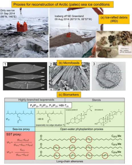
Figure 6.Proxies for reconstruction of Arctic (paleo) sea ice conditions and sea‐surface temperature (SST). (a) Ice‐rafted debris, (b) examples of microfossils (from left to right: modern sea‐ice algae/Brown et al., 2014; Eocene sea‐ice algae/
Stickley et al., 2009; dinocystIslandinium minutum/de Vernal & Rochon, 2011), and (c) specific biomarkers indicative for sea ice cover ("IP25"), phytoplankton open‐water productivity (specific sterols, highly brached isoprenoids (HBIs), and long‐chain alkenones) and SST. By combining IP25and open‐water phytoplankton biomarkers (“PIP25”; cf. Müller et al., 2011) or specific HBIs (“HBI‐T25”; cf. Belt et al., 2019), even information about temporal and spatial changes in sea‐ice coverage can be obtained (for further details, see text).
Sea ice often contains large amount of terrigenous material that has been entrained into the ice in the mar- ginal seas (sediment‐laden or“dirty”sea ice; Figure 6a; e.g., Pfirman et al., 1989; Nürnberg et al., 1994;
Eicken et al., 1997, Eicken et al., 2005; Dethleff et al., 2000). In areas of sea‐ice melting, sediment particles are released and deposited at the seafloor, contributing significantly to the present and past Arctic Ocean sedimentary budget. This sea‐ice sediment—or“ice‐rafted debris (IRD)”—mainly consists of terrigenous material with clay minerals, quartz, feldspars, heavy minerals, and specific Fe oxide grains as the main com- ponents. The mineralogy of sea‐ice sediments may be very variable in time and space, depending on the geol- ogy of the source areas in the hinterland. Thus, studies of the mineralogical composition may allow the identification of source areas of the IRD particles and, based on these data, the reconstruction of past and present transport pathways (e.g., Nürnberg et al., 1994; Wahsner et al., 1999; Darby, 2003, 2014; see Stein, 2008 for review). IRD, however, can also be transported by icebergs (Figure 6a). If IRD is related to iceberg transport and not sea ice, the IRD proxy records the existence of extended continental ice sheets reaching the shelf‐break. Here afirst‐order proxy to discriminate between sea‐ice and iceberg‐rafted sediments is the grain‐size distribution. It is generally accepted that very coarse‐grained material >250μm up to pebble size (Figure 6a) are mainly restricted to iceberg transport, whereas the dominance offiner‐grained (silt and clay) sediments are more typical for sea‐ice transport (e.g., Clark & Hanson, 1983; Nørgaard‐Pedersen et al., 1998;
Spielhagen et al., 2004; Dethleff, 2005).
Sea‐ice associated organisms like pennate ice diatoms are frequently used for reconstructing present and past sea‐ice conditions (e.g., Koç et al., 1993; Stickley et al., 2009). However, it has also been shown that the preservation of fragile siliceous diatom frustules can be relatively poor in surface sediments from the Arctic realm, and the same is also true (if not worse) for calcareous‐walled microfossils, thus limiting their applicability (Matthiessen et al., 2001; Schlüter et al., 2000; Steinsund & Hald, 1994). De Vernal, Rochon, et al. (2013) present a status report about reconstructing past sea‐ice cover of the Northern Hemisphere using dinoflagellate cysts. Based on a study of Arctic Greenland shelf sediments, Limoges et al. (2018) provide new insights into the distribution of a sea ice‐associated dinoflagellate species, speciesPolarella glacialisand its cysts, and propose that this species might have the potential to become a useful proxy for reconstructing past seasonal sea ice.
A multiproxy approach considering sediment texture in combination with lithology and sediment prove- nance as well as micropaleontological and geochemical data indicative for surface‐water characteristics cer- tainly provides a much sounder interpretation of sea‐ice versus iceberg‐rafted sediments and reconstruction of past sea‐ice conditions.
The ability to (semi‐)quantitatively reconstruct paleo‐sea‐ice distributions has been significantly improved by a biomarker approach based on determination of a highly branched isoprenoid (HBI) with 25 carbons (C25
HBI monoene—“IP25”; Figure 6c; Belt et al., 2007). This biomarker is only biosynthesized by specific diatoms living in Arctic sea ice (Figure 6b; Brown et al., 2014); that is, its presence in the sediment is a direct proof of the presence of past Arctic sea ice. Furthermore, IP25appears to be a specific, sensitive, and stable proxy for Arctic sea ice in sedimentary sections representing late Miocene to Holocene times (Belt, 2018; Belt & Müller, 2013; Knies et al., 2014; Stein et al., 2012, 2016, and references therein). When using this proxy, however, one has to consider that IP25is more or less absent under a permanent sea‐ice cover that limits light penetration and, in consequence, sea‐ice algal growth. The same consequence applies to totally ice‐free conditions where no ice algae live, that is, IP25= 0. This difficulty in interpreting IP25data can be overcome by the additional use of phytoplankton‐derived, open‐water biomarkers such as brassicasterol and dinosterol (Müller et al., 2009, 2011) or specific tri‐unsaturated HBIs (Belt et al., 2015, 2019; Limoges et al., 2018; Ribeiro et al., 2017; Smik et al., 2016). By combining the environmental information carried by IP25and the different phy- toplankton biomarkers (Figure 6c), even more semiquantitative estimates of present and past sea‐ice cover- age, seasonal variability, and marginal ice zone situations are possible (Müller et al., 2011; Belt et al., 2015, 2019; Stein et al., 2017; for recent and critical review of this biomarker approach, see Belt, 2018).
Another useful option to distinguish between the two“IP25= 0”extremes, that is, ice‐free versus thick closed ice coverage, is the determination of SST. SST values significantly above 0 °C give important information about surface water characteristics per se, but also clearly point to ice‐free conditions if IP25= 0. For recon- structions of past SST conditions in the central Arctic Ocean during the Cretaceous, Paleocene‐Eocene and Miocene, very promising biomarker SST tools such as the alkenone‐based UK37index (Brassell et al., 1986;
Prahl & Wakeham, 1987) and the TEX86index (Schouten et al., 2002, 2004) have been used successfully (Jenkyns et al., 2004; Sluijs et al., 2006, Sluijs et al., 2009; Weller & Stein, 2008; Stein, Weller, et al., 2014;
for further discussion, see below).
The alkenone‐based UK37 approach evolved from the observation that certain microalgae of the class Prymnesiophyceae, notably the marine coccolithophorids Emiliania huxleyi and Gephyrocapsa oceanica (e.g., Conte et al., 1992; Marlowe et al., 1984; Volkman et al., 1980), and presumably other living and extinct members of the familyGephyrocapsae(Marlowe et al., 1990; Müller et al., 1998), have or had the capability to synthesize alkenones whose extent of unsaturation changes with growth temperature (Brassell et al., 1986;
Marlowe et al., 1984; Prahl & Wakeham, 1987). Based on this correlation, paleo‐SST can be calculated from the so‐called ketone unsaturation index UK37or the simplified version of the index UK37′(Figure 6c; Brassell et al., 1986; Prahl & Wakeham, 1987; Müller et al., 1998). The TEX86approach is based on specific membrane lipids, that is, tetraether lipids (glycerol dialkyl glycerol tetraethers) with 0–4 cyclopentane rings and, in one case, a cyclohexane ring, synthesized by marineCrenarchaeota(Schouten et al., 2002). As shown in a study of marine surface sediments from the world oceans, these organisms adjust the composition of these tetra- ether lipids in response to SST (Ho et al., 2014; Kim et al., 2008; Schouten et al., 2002, 2004; Weijers et al., 2006; Wuchter et al., 2004). This response is quantified as the so‐called TEX86 (tetraether index of 86 carbon atoms).
5. Long‐Term Climate Change From Greenhouse to Icehouse Conditions
The Mesozoic to Cenozoic time interval is a period when the climate on Earth changed from one extreme (Cretaceous‐Paleogene Greenhouse lacking major ice sheets) to another (Neogene Icehouse with bipolar glaciation; Figure 7; Pearson & Palmer, 2000; Norris et al., 2002; Zachos et al., 2008; Friedrich et al., 2012;
Kent & Muttoni, 2013; O'Brien et al., 2017; O'Connor et al., 2019). This long‐term climatic evolution, includ- ing prominent warm and cold phases, is best reflected in marine deep‐water and surface‐water temperatures determined from benthic and planktic oxygen isotope, Mg/Ca thermometry, and biomarker (TEX86and UK37) records, respectively, from low to middle latitudes (e.g., Alsenz et al., 2013; Bijl et al., 2009;
Friedrich et al., 2012; Lear et al., 2000; Littler et al., 2011; Liu et al., 2009; Miller et al., 1987; Mutterlose et al., 2010; O'Brien et al., 2017; Zachos et al., 2001; Zachos et al., 2008). Peak warm intervals occurred around the Cenomanian/Turonian boundary, during the Paleocene‐Eocene Thermal Maximum (PETM), the Early Eocene Climate Optimum (EECO), and the Middle Eocene Climate Optimum (Figure 7), most probably related to higher atmospheric CO2concentrations. The long‐term, post‐EECO high‐latitude cool- ing started near 50 Ma and is punctuated by four major steps in the early mid‐Eocene (about 48–45 Ma), at the Eocene/Oligocene boundary (near 34 Ma), in the mid‐Miocene (at about 14 Ma), and in the mid‐
Pliocene (at about 3.5–2.6 Ma; Figure 7; Miller et al., 1987; Lear et al., 2000; Pearson & Palmer, 2000;
Zachos et al., 2001, Zachos et al., 2008; Westerhold & Röhl, 2009). Furthermore, long‐term climatic changes on global and regional (e.g., Arctic) scales are also controlled by plate tectonic processes such as opening and closure of oceanic gateways, isolating single ocean basins from the World Ocean, configuration of conti- nents, and uplift of mountain ranges and plateaus (Hay et al., 1999; Scotese, 2001; Müller et al., 2008; refer- ences with focus on the Arctic Ocean: Kristoffersen, 1990; Grantz et al., 2011; Shephard et al., 2013; Kanao et al., 2015; Petrov et al., 2016).
The long‐term paleoclimatic and paleoceanographic history of the Arctic Ocean through this time interval, however, is still poorly known in comparison to other world ocean areas. Major information on the paleoen- vironment of the early Arctic is derived from circum‐Arctic terrestrial data sets (for references, see next sec- tions) and—concerning the marine records—from petroleum exploration drill holes from the Arctic marginal seas (e.g., Leith et al., 1992; Spencer et al., 2011) and Deep‐Sea Drilling Project and ODP drill cores from subarctic regions (Leg 38: Talwani et al., 1976; Leg 104: Eldholm et al., 1989; Leg 105: Srivastava et al., 1989; Leg 151: Thiede et al., 1996; Leg 152: Larsen et al., 1994; Leg 162: Raymo et al., 1999; see Figure 1 for locations). Direct information from sediment cores derived from the central Arctic Ocean is restricted to a very few short sections—at least prior to the IODP‐ACEX drilling campaign in 2004 (Figure 7; Thiede et al., 1990; Backman et al., 2008; see below). From Figure 7 it is obvious that for almost the entire Miocene, the Oligocene, Eocene, and Paleocene, no sediment‐core data are available at all. For the Cretaceous, data from
central Arctic Ocean cores are limited to three short sections representing isolated, discontinuous fragments of the late Campanian and Maastrichtian climate history (see next section).
5.1. The Cretaceous Arctic Ocean: Warm, Euxinic, and Productive, but Occasionally Ice
Up to the 1980s, the general global climate of the Cretaceous was viewed as a period of great warmth over the entire globe (Frakes, 1979; Hallam, 1985). According to these authors, tropical‐subtropical conditions pre- vailed to at least 45°N and possibly to 70°S, and warm to cool‐temperate climates extended to the ice‐free polar regions. Such a greenhouse world was characterized by significantly higher temperatures and reduced latitudinal temperature gradients (O'Brien et al., 2017; Robinson et al., 2019; Sinninghe Damsté et al., 2010).
The overall warm climatic conditions most likely resulted from an enhanced greenhouse effect due to higher atmospheric CO2concentrations as inferred from various proxies (Figure 7; Crowley & Berner, 2001; Royer, 2010; Kent & Muttoni, 2013; Foster et al., 2017) and conventionally attributed to the balance between the input of CO2 from ocean crust production, volcanism, metamorphism, and organic carbon weathering and the output of CO2 from silicate weathering and organic carbon burial (Foster et al., 2017; Kent &
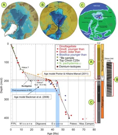
Muttoni, 2013; Walker et al., 1981; Weissert & Erba, 2004). During the 1990s, however, the view of constant equable warmth and sluggish oceanic circulation during the Cretaceous was questioned, and much more Figure 7.(a) Stratigraphic coverage of existing sediment cores in the central Arctic Ocean prior to IODP‐ACEX (2004) over the last 100 Ma, including the four short cores representing short sections of Eocene and/or Maastrichtian/Campanian sediments (Backman et al., 2008; Stein et al., 2015; Thiede et al., 1990) and one core representing late Miocene sediments (Stein, 2015; Stein et al., 2016). Red question marks indicate time interval with no information. (b) The stratigraphic range of the sedimentary section recovered during the ACEX drilling expedition used on the two age models by Backman et al. (2008; AM‐1) and Poirier and Hillaire‐Marcel (2011; AM‐2). (c) Globalδ18O stack of benthic foraminifera for the past 100 million years representing the Greenhouse‐Icehouse transition (Friedrich et al., 2012; Zachos et al., 2008). CTM = Cretaceous Thermal Maximum (Cenomanian/Turonian boundary); C/T = Cretaceous/Tertiary Boundary; PETM
= Paleocene‐Eocene Thermal Maximum; EECO = Early Eocene Climate Optimum; MECO = Middle Eocene Climate Optimum; Oi‐1 = Major Oligocene Glaciation Event; MMCO = Middle Miocene Climate Optimum. (d) Single data points and smoothed record (red line) of atmospheric CO2estimates from various proxies (see different symbols), based on compilations by Royer (2010) for the pre‐70‐Ma interval and by Beerling and Royer (2011) for the post‐70‐Ma interval (Kent
& Muttoni, 2013, supplemented). Red stippled lines indicate atmospheric CO2levels of 278 (preindustrial value) and 450 ppm, respectively.
variable climatic conditions were suggested for this time period (e.g., Kemper, 1987; Miller et al., 2005;
Mutterlose et al., 2003; Price et al., 2000; Weissert & Lini, 1991). Even if warm climates in the high latitudes dominated much of the Cretaceous (to early Eocene) and warmth may have been caused by high CO2, short intervals of more restricted glaciations probably occurred (at least) on Antarctica (Miller et al., 2005). These authors propose a vision of Earth's cryospheric evolution that reconciles warm, generally ice‐free poles with cold snaps that resulted in glacio‐eustatic lowerings of 20–40 m, probably driven by orbital forcing (Matthews & Frohlich, 2002; DeConto & Pollard, 2003; for general review and references, see Haq, 2014).
The availability of nutrients and elevated atmospheric CO2may have stimulated primary production, which is thought to be one of the main factors (besides bottom‐water stagnation) causing anoxic conditions in large parts of the oceans (e.g., Arthur et al., 1984, 1987; de Graciansky et al., 1984; Demaison & Moore, 1980;
Erbacher et al., 2001; Ohkouchi et al., 2015; Schlanger & Jenkyns, 1976). These major episodes are known as“oceanic anoxic events”(Schlanger & Jenkyns, 1976) and represent major perturbations in the global cli- mate and ocean system defined by massive organic carbon (OC) burial and black shale formation in marine environments. Oceanic anoxic events occurred on a regional to worldwide scale with the most prominent and widespread ones in the Toarcian, the Valanginian, the Aptian‐Albian, the Cenomanian‐Turonian, and the Coniacian‐Santonian (Arthur et al., 1984, 1987; Brumsack, 1980; de Graciansky et al., 1984; Erba et al., 2004, 2015; Erba et al., 2019; Gambacorta et al., 2016; Méhay et al., 2009; Ohkouchi et al., 2015;
Rais et al., 2007; Schlanger & Jenkyns, 1976; Stein et al., 1986). Upper Jurassic to Cretaceous black shales were also deposited in all the large circum‐Arctic sedimentary basins (e.g., North Alaskan Basin, Mackenzie Delta Basin, Sverdrup Basin, Barents Shelf, and western Siberia) that are highly productive in terms of gas and oil (e.g., Bakke et al., 1998; Dixon et al., 1992; Leith et al., 1992; Lenniger et al., 2014;
Spencer et al., 2011).
A dominantly warm climate probably existed in the Northern High Latitudes during Middle to Late Cretaceous times as indicated by the presence of deciduous trees and leaves with characteristic morpholo- gies, at 80–85°N (Herman & Spicer, 1996; Parrish & Spicer, 1988; Spicer & Herman, 2010), the presence of crocodiles beyond 60°N (Markwick, 1998), and most specifically, the discovery of champosaurs (cold‐
blooded reptiles; closest living relatives are crocodiles) in the Turonian of the Sverdrup Basin (Axel Heiberg Island) at 72°N paleolatitude (Tarduno et al., 1998; Huber, 1998; for summary, see O'Regan et al., 2011). Besides indication for a relatively warm (sub‐) Arctic climate during Cretaceous times, there are also signals pointing to cold climatic conditions. In particular for parts of the Early Cretaceous, hints of Icehouse conditions or at least cool climates in the higher latitudes were found. Glendonites (pseudomorphs of the low‐temperature hydrated form of calcium carbonate, ikaiite) found in lower Valanginian and upper Aptian sediments from the Sverdrup Basin in Arctic Canada (70–80°N paleolatitude) imply that Early Cretaceous seawater temperatures were at times close to freezing (Kemper, 1987). Almost certainly these cooler temperatures record global changes because, at least in the case of the late Aptian, coeval glendonites are also known from the Southern Hemisphere, found in the Eromanga Basin in Australia at a paleolatitude of 65°S (De Lurio & Frakes, 1999; Frakes & Francis, 1988). Furthermore, Frakes and Francis (1988) postulate at least seasonally cold ocean temperatures and limited polar ice caps for the Early Cretaceous from the occurrence of ice‐rafted deposits in Siberia, Australia, and Spitsbergen. Nannofossil assemblages from off- shore mid‐Norway and the Barents Sea also suggest cold conditions (Mutterlose et al., 2003; Mutterlose &
Kessels, 2000). Based on oxygen stable isotope paleothermometry of well‐preserved Middle Jurassic to Lower Cretaceous belemnites from Kong Karls Land, Svalbard, cool high‐latitude marine paleotemperatures of <8 °C were estimated for the early to middle Valanginian, which may be compatible with the formation of high‐latitude ice (Ditchfield, 1997).
What about marine sedimentary records from the Arctic Ocean representing information about climatic conditions during (late Jurassic to) Cretaceous times, that is, at times when the Arctic Ocean was probably much more isolated from the world ocean in terms of deep‐water connection (Figure 8)? The isolation of the Arctic Ocean at those times was an important prerequisite for the development of widespread anoxic/euxinic conditions during the Late Jurassic/Early Cretaceous (e.g., Spencer et al., 2011). As already mentioned above, most of the sedimentological, micropaleontological, and geochemical data available for paleoenvironmental reconstructions of the Arctic realm during this time interval are from petroleum exploration drill holes from the marginal seas such as the Barents Sea and along the Norwegian continental
margin (Figure 8), whereas data from the central Arctic Ocean are restricted to a few short sediment cores (Figure 9; see below).
In the southern Barents Sea, for example, OC‐rich sediments of Late Jurassic/Early Cretaceous age were recovered, characterized by OC contents of up to about 35% (Figure 8; Langrock et al., 2003a). High hydrogen‐index values of 400–600 mg HC/g C obtained by Rock‐Eval pyrolysis (Langrock et al., 2003a) and maceral compositions of the sediments dominated by lipid‐rich organic matter derived from mainly marine but also brackish and freshwater algae (“alginites”) as well as fine‐grained “liptodetrinites” (Figure 8) support a type II kerogen characterization. The excellent preservation of the labile, easily degrad- able organic matter particles and the significant amounts of freshwater algae argue for deposition in a restricted shallow basin very close to land rather than an upwelling regime (Arthur et al., 1987; Taylor et al., 1998). The increasing OC content in the late Volgian section was most likely caused by a combination of increasing preservation by bottom‐water anoxia, coupled with periods of increasing primary production as well as a low and decreasing dilution of clastic material, related to a marked rise in sea level (Figure 8;
Langrock et al., 2003a). During the Late Jurassic and Early Cretaceous, such anoxic conditions proposed for large parts of the proto‐Arctic Ocean, probably extended toward the south into the Norwegian‐ Greenland Sea as shown in geochemistry and microscopy data sets from black shale sequences recovered in drill cores along the Norwegian shelf (Figure 8; Langrock et al., 2003b; Langrock & Stein, 2004). The high abundance of autochthonous small‐sized pyrite framboids indicative for an anoxic water column (i.e., under euxinic conditions), such as typical for the modern Black Sea (cf. Wilkin et al., 1997), the carbon‐sulfur‐iron Figure 8.(a) Paleogeographic map for the Valanginian (lowermost Cretaceous) from Africa to the Arctic, showing transcontinental seaways, major marine embay- ments and basins, and selected cores west and north of Norway (Mutterlose et al., 2003). Core 7430/10‐U‐01 is marked as a red circle. (b) Core depth,
stratigraphic correlation, lithology, regional formational limits, and total organic carbon (TOC) record of the interval between 67 and 32 mbsf of Core 7430/10‐U‐01.
For the TOC‐rich interval between 49 and 55 mbsf, organic matter composition has been determined in detail by means of maceral analysis. For maceral analysis, small blocks of rock (3–4 cm3) were collected perpendicular to the bedding andfixed by a cold‐setting epoxy resin, polished, and analyzed by point‐ counting with a 25‐point ocular grid using a Zeiss Axiophot microscope under incident andfluorescence light (cf. Langrock et al., 2003a). The records were cor- related and interpreted in relationship to the global sea‐level curve of Haq et al. (1988). Photograph of afinely laminated section showing layers of algae‐type organic matter (yellow color due tofluorescence light) andfish remains, alternating with nonorganic siliciclastic layers (black). The cartoon illustrates the interpretation of organic‐carbon data in terms of paleoenvironmental situation (Langrock et al., 2003a, supplemented).
relationships (cf.Hofmann et al., 2000 ; Lückge et al., 1996), the high concentrations of Mo, and the Re/Mo ratios also support widespread euxinic conditions (Langrock et al., 2003a, 2003b; Lipinski et al., 2003).
In addition, patchily distributed, coarse‐grained minerals (apparently quartz) are found, which are 60 to 200 μm in diameter (Figure 8). These minerals could not have been transported along with the claystone facies.
Here a possible mechanism for the input of these large sand grains was ice rafting. Episodes of a relatively cool climate were already suggested for the earliest Cretaceous Boreal realm as described above. Hence, epi- sodic (or even seasonal) IRD input might have occurred in the late Volgian Barents Sea (Figure 8) at a paleo- latitude of almost 55°N (Langrock et al., 2003a).
In the central Arctic Ocean, Cretaceous sediments were only cored at three locations on the Alpha Ridge:
cores Fl‐437 and Fl‐533 taken during the drift of the ice‐island T‐3 from 1963 to 1974 and Core CESAR‐6 of the Canadian Expedition to Study the Alpha Ridge (CESAR) in 1983 (Figure 9a; Thiede et al., 1990). In 2004, an about 3‐m‐thick interval of Campanian very dark gray clayey mud and silty sands with OC values of about 1–2% was recovered in the lowermost part of the ACEX record from Lomonosov Ridge (Backman et al., 2006; Stein, 2007). During the FRAM‐2014/2015 Ice Drift Expedition (Kristoffersen et al., 2016;
Kristoffersen & Tholfsen, 2016), a 300‐m‐thick sequence offlat‐lying Cenozoic sediments overlying dipping (probably) Mesozoic sediments, separated by an unconformity, were recognized in a seismic reflection pro- file across Lomonosov Ridge close to the North Pole (the age classification proposed by the authors is based on comparison with the ACEX drilling results). A gravity corer was dropped down where the potential for exposure of sedimentary rocks below the unconformity was high, and, as result, a short core (FRAM14/
15‐2) containing a“20 cm thick section of very cohesive, light cream colored sediments–something we have not seen so far from the Arctic Ocean”was recovered (Kristoffersen & Tholfsen, 2016; see Figure 9a for core Figure 9.(a) Map showing the late Cretaceous paleogeography of the Arctic region with the Alpha Ridge and the locations of sites CESAR‐6 (C6) and FL‐533, and the locations of the English Chalk and Boreal Chalk Sea (Stevns‐1 Core) sections; inset shows modern geography and locations of cores CESAR‐6, FL‐437 and Fl‐533 (Alpha Ridge), the ACEX site (Lomonosov Ridge), Core FRAM14/15‐2 (Lomonosov Ridge), and Core 7430/10‐U‐01 (Barents Sea). (b) Core CESAR‐6:
Backscattered Electron Image of resin‐embedded sediment showing darker diatom vegetative cell laminae, interbedded with paler layers composed primarily of diatom resting spores, and enlargements of representative topographic SEM images of the diatom vegetative cells and the diatom resting spores, and thin laminae of poorly sorted terrigenous sediment occurring dominantly within the spring diatom bloom layer, interpreted as evidence for ice‐rafted debris (IRD; Davies et al., 2009). (c) TEX86values and related SST values (Jenkyns et al., 2004), and organic carbon, hydrogen index values, and lithologies of the lowermost upper Cretaceous section of Core FL‐533 (data from Clark et al., 1986; Firth & Clark, 1998).
location). These sediments are almost pure siliceous oozes composed of well‐preserved diatoms, radiolar- ians, silicoflagellates, etc. (first observations by R. Stein, unpubl. data, 2019). More detailed work by micro- paleontologists on the species identification and age determination (Campanian/Maastrichtian? or younger?) are in process now; thus, no further discussion is presented at this stage.
At Core CESAR‐6, siliceous, well‐laminated Campanian‐Maastrichtian sediments with excellently pre- served microfossils were retrieved (Jackson et al., 1985). Very similar sediments of Campanian age were also recovered at Core Fl‐437: a yellowish laminated siliceous ooze rich in diatoms, ebrideans, silicoflagellates, and archaeomonads with sparsefish remains (Clark et al., 1986; Dell'Agnese & Clark, 1994). More recently, Davies et al. (2009), Davies et al., 2011) analyzed in detail the laminated section of Core CESAR‐6 using
“backscattered electron imagery” and identified a seasonal succession of two distinct lamina types that represent an annual lamina couplet (Figure 9b). Type A of laminae consists of diatom resting spores repre- sentingflux from the spring bloom, and type B of laminae consists of diatom vegetative cells representing flux from production during the stratified months of the Arctic summer (Davies et al., 2011). In some of these lamina couplets, coarse‐grained terrigenous particles (mainly quartz) indicative of ice‐rafting (IRD) were found (Figure 9b). The diatom laminae point to a strong seasonality, that is, to ice‐free summers, whereas the presence of IRD is interpreted as a signal for sea ice that occasionally may have occurred during severe winters (Davies et al., 2009; Davies et al., 2011).
In Core Fl‐533, the lowermost 67 cm of the 348‐cm‐long sequence comprise OC‐rich black mud (black shales) of early Maastrichtian age (Clark et al., 1986; Firth & Clark, 1998). These black shales are character- ized by very high OC contents of up to almost 16% and hydrogen index values of about 250 to 350 mg HC/g OC (Figure 9c), indicating an immature, mixed marine‐terrigenous type of organic matter with major con- tributions from marine/aquatic algae. That means, both OC content and composition were totally different in comparison to those within the Quaternary deposits (Stein et al., 2001; Stein & Macdonald, 2004).
Whereas the OC buried and preserved in Quaternary sediments is mainly refractory terrigenous matter, the OC found in the Cretaceous sediments mainly consists of labile algae‐type organic matter. These data suggest that the Cretaceous Arctic Ocean basin may have been an important sink for algae‐type OC (and CO2) and, thus, of importance for the global climate system of that time.
In order to get some information about the Cretaceous SST of the central Arctic Ocean, Jenkyns et al. (2004) used the TEX86approach (Schouten et al., 2002; see section 4) and analyzed black shale samples from Core Fl‐533 for membrane lipids of marine Crenarchaeota (Figure 9c). The TEX86results indicate an average Arctic Ocean SST of 15 ± 1 °C at a paleolatitude of about 80°N for that part of the early Maastrichtian repre- sented by the black muds (Figure 9c). Considering the diatom and IRD data from the CESAR‐6 Core (see above), this SST of about 15 °C should certainly represent summer conditions. A summer SST of about 15
°C and the presence of sea ice during winter may represent conditions similar to those described for the Eocene central Arctic Ocean (see section 5.2).
5.2. The Early Cenozoic Transition: Euxinic Conditions and Onset of Arctic Sea Ice
For the Arctic Ocean, information about the early Cenozoic climate history is quite limited (cf. Figure 7). A large amount of information is based on paleobotanic studies of circum‐Arctic terrestrial outcrops. As reported from several localities around the Arctic Ocean such as Axel Heiberg Island, Ellesmere Island, Mackenzie Delta, Alaska, and the New Siberian Islands,floral and faunal assemblages indicate exceptionally warm and humid conditions during the late Paleocene‐early Eocene (Basinger et al., 1994; Dolezych et al., 2018; Eberle et al., 2010; Eldrett et al., 2009; Greenwood et al., 2010; Salpin et al., 2018; Suan et al., 2017;
West et al., 2015). Multiproxy data from early Eocene deltaic plain sediments of the Mackenzie Delta (Arctic Canada near 75°N), for example, indicate annual air temperatures averaging 21–22 and 10–14 °C in winter (Salpin et al., 2018). Late Paleocene mean annual shallow‐marine temperatures between 11 and 22 °C were recorded from mollusk stable isotopes determined in sediments from the Prince Creek Formation (Alaska, 80°N; Brice et al., 1996). Direct information about paleoenvironmental conditions in the central Arctic Basin prior to the ACEX drilling in 2004 was coming from a single short sediment core obtained from the drifting ice island T3 in 1969 (Core FL‐422; see Figure 9a for location). The sediments of this core representing part of the middle Eocene time interval are laminated, rich in siliceous microfossils, especially diatoms and silicoflagellates, and characterized by alternating layers of vegetative cells and resting spores, interpreted as evidence for strong seasonality, upwelling of nutrient‐rich waters, and warm surface‐
water temperatures (Bukry, 1984; Clark, 1974; Dell'Agnese & Clark, 1994). As mentioned in the previous section, similar sediments with excellently preserved siliceous microfossils were also found in Core FRAM14/15‐2 recovered from Lomonosov Ridge during the FRAM‐2014/2015 Ice Drift Expedition (Kristoffersen & Tholfsen, 2016; Kristoffersen et al., 2016; for core location, see Figure 9a). However, the age of this sedimentary section (i.e., Campanian/Maastrichtian vs. Eocene) has not been determined yet.
With the ACEX drilling in 2004, a thick sequence of upper Cretaceous to Quaternary sediments became avail- able for paleoclimatic reconstructions (Figure 10; Backman et al., 2006; Moran et al., 2006). These sediments are characterized by prominent changes in sediment composition and texture, suggesting drastic paleoenvir- onmental changes through time (Backman et al., 2006; Stein, 2007). Whereas the lower half of the ACEX sequence (Units 2 to 4) mainly consists of dark gray silty clay and biosiliceous ooze characterized by high TOC values of 1% to >5%, the upper half of the ACEX sequence (subunits 1/1 to 1/4) is composed of silty clay with very low TOC contents of <0.5% (Figure 11a), that is, values very similar to those known from upper Quaternary records determined in gravity cores from the Lomonosov Ridge and representing modern‐type oxic deep‐water conditions (Stein et al., 2001). In subunit 1/5 (about 193 to 199 m of composite depth (mcd)) characterized by distinct gray/black color bandings (“Zebra Unit“), TOC maxima of 7% to 14.5%
Figure 10.Age‐depth diagram and main lithological units of the ACEX section (O’Regan, 2011, supplemented), based on the biostratigraphically derived age model by Backman et al. (2008) and the alternate chronology based on osmium isotopes (Poirier & Hillaire‐Marcel, 2011). Depth offirst occurrence of IRD between 240 and 260 mcd are marked as light blue horizontal bar. On top (a) International Bathymetric Chart of the Arctic Ocean (Jakobsson et al., 2012) repre- senting modern boundary conditions with connections to the world ocean; (b) paleogeographic/paleobathymetric reconstruction for the late early Miocene. BSG = Barents Sea Gateway; JM = Jan Mayen Microcontinent; KR = Knipovich Ridge; MJ = Morris Jessup Rise; NS = Nares Strait; YP = Yermak Plateau (Jakobsson et al., 2007), and (c) Paleogeography of the Arctic region for the early middle Eocene during the phase of high biosilica production and preservation and euxinic conditions (50–45 Ma; Stickley et al., 2009). The location of the ACEX site is marked as a red circle.
were measured (Stein, 2007). The Eocene section (about 200 to 385 mcd) characterized by high (algae‐type) organic carbon content is mainly related to euxinic conditions predominant at that time when the Arctic Ocean was quite isolated from the world ocean (Figures 10 and 11; Backman et al., 2006; Stein et al., 2006, Stein, Weller, et al., 2014). The transition from euxinic conditions to the modern‐type oxic conditions occurred during Oligocene‐Miocene times and is related to the opening of Fram Strait, allowing the inflow of oxygen‐rich deep water from the Atlantic into the Arctic Ocean (Jakobsson et al., 2007).
The exact timing of this prominent environmental change, that is, 17.5 versus 32 Ma, however, is still under debate and depends on the age model that is used, that is, Backman et al. (2008) versus Poirier and Hillaire‐
Marcel (2011); Figure 10). Backman et al. (2008) stratigraphic framework of the Cenozoic ACEX sequence is based on biostratigraphic, cosmogenic isotope, magneto‐and cyclostratigraphic data, and they proposed a major hiatus spanning the time interval from 44.4 to 18.2 Ma. When following this age model, a large part of the climate history covering the transition from Greenhouse to Icehouse is missing in the ACEX Figure 11.(a) Record of total organic carbon (TOC) contents as determined in the composite ACEX sedimentary sequence (Stein, 2007). Data on lithological units (LU) and core recovery (Rec.) from Backman et al. (2006). Age models AM‐1 (Backman et al., 2008) and AM‐2 (Poirier & Hillaire‐Marcel, 2011) are shown. The“Zebra”Unit (Unit 1/5) marks the transition from an euxinic ocean to an oxygenated ocean that occurred when the formerly isolated Arctic Ocean became connected to the world ocean via Fram Strait (cf. Figure 10). Depending on the age model, this transition is in the mid‐Miocene (17.5 Ma) or Oligocene (32 Ma). Cam = Campanian; LP = late Paleocene; Mid Mioc. = middle Miocene; L.Pl. = late Pleistocene. (b) Record of terrigenous sand (150–250μm) interpreted as ice‐rafted debris (IRD); blue circles mark occurrence of pebble‐sized IRD (based on St. John, 2008). The onset of glaciation is marked as light blue bar.
Photographs show coarse fraction >250μm (IRD) in two samples from 240.39 and 21.4 m composite depth (mcd), respectively.