Simulation of QCD with N

JHEP02(2015)043

Published for SISSA by Springer Received: November 18, 2014 Accepted: January 9, 2015 Published: February 6, 2015

Simulation of QCD with N

= 2 + 1 flavors of non-perturbatively improved Wilson fermions

Mattia Bruno,^a Dalibor Djukanovic,^b Georg P. Engel,^c Anthony Francis,^b Gregorio Herdoiza,^d Hanno Horch,^e Piotr Korcyl,^a Tomasz Korzec,^f Mauro Papinutto,^g Stefan Schaefer,^a Enno E. Scholz,^h Jakob Simeth,^h Hubert Simma^a and Wolfgang S¨oldner^h

aJohn von Neumann Institute for Computing (NIC), DESY, Platanenallee 6, D-15738 Zeuthen, Germany

bHelmholtz Institute Mainz, University of Mainz, D-55099 Mainz, Germany

cDipartimento di Fisica, Universit`a di Milano-Bicocca, and INFN, Sezione di Milano-Bicocca, Piazza della Scienza 3, I-20126 Milano, Italy

dDepartamento de F´ısica Te´orica and Instituto de F´ısica Te´orica UAM/CSIC, Universidad Aut´onoma de Madrid,

Cantoblanco, E-28049 Madrid, Spain

ePRISMA Cluster of Excellence, Institut f¨ur Kernphysik, Johannes Gutenberg Universit¨at Mainz,

D-55099 Mainz, Germany

fInstitut f¨ur Physik, Humboldt Universit¨at, Newtonstr. 15, D-12489 Berlin, Germany

gDipartimento di Fisica, “Sapienza” Universit`a di Roma, and INFN, Sezione di Roma, P.le Aldo Moro 2, I-00185 Roma, Italy

hInstitut f¨ur Theoretische Physik, Universit¨at Regensburg, D-93040 Regensburg, Germany

E-mail: stefan.schaefer@desy.de

Abstract:We describe a new set of gauge configurations generated within the CLS effort.

These ensembles have Nf = 2 + 1 flavors of non-perturbatively improved Wilson fermions in the sea with the L¨uscher-Weisz action used for the gluons. Open boundary conditions in time are used to address the problem of topological freezing at small lattice spacings and twisted-mass reweighting for improved stability of the simulations. We give the bare parameters at which the ensembles have been generated and how these parameters have been chosen. Details of the algorithmic setup and its performance are presented as well as measurements of the pion and kaon masses alongside the scale parametert0.

Keywords: Lattice QCD, Lattice Gauge Field Theories ArXiv ePrint: 1411.3982

JHEP02(2015)043

Contents

1 Introduction 2

2 Physical parameters 3

2.1 Action 3

2.2 Choice of parameters 4

2.3 Quark mass trajectory 5

2.4 Tuning strategy 6

3 Algorithmic parameters 6

3.1 Twisted-mass reweighting 6

3.2 Determinant factorization 8

3.3 RHMC 8

3.4 HMC and the integration of the molecular dynamics 10

3.5 Solver 11

3.6 Production cost 11

4 Autocorrelations 12

4.1 Scaling of the autocorrelations 13

4.2 Cost of the simulation 13

5 Reweighting factors 14

5.1 Twisted-mass reweighting factor 14

5.2 Reweighting and the pseudoscalar correlation function 15

5.3 Computation of W₀ 15

5.4 RHMC reweighting factor 16

6 Observables 17

6.1 Wilson flow 17

6.2 Effects of the boundary 18

6.3 Measurement of t0 19

6.4 Pseudoscalar masses 20

6.5 Comparison to simulations with periodic boundary conditions 21

7 Scaling violations 22

7.1 Cutoff effects int₀ 22

7.2 Coarser lattices 23

8 Conclusions 24

JHEP02(2015)043

1 Introduction

What can be achieved in lattice QCD computations in terms of observables and their accuracy depends to a large extent on the availability of suitable ensembles of gauge field configurations. For reliable results, many sources of error have to be controlled: fine lattices are needed for minimal discretization effects, the quark masses have to be close to their physical values and the volume of the lattices has to be large enough for finite size effects to be small. The final precision also depends on the quark flavor content of the sea. On top of these systematic effects come statistical uncertainties: simulations have to be long enough such that the statistical errors can be estimated reliably, and with statistical uncertainties getting smaller, the need for control over systematic effects increases.

Since the generation of gauge field configurations is computationally the most demand- ing part of the whole computation, a careful evaluation of the physics parameters needs to be made in view of the target precision of the observables — as far as this is possible at this stage. The goal is to balance the various sources of systematic and statistical uncertainties in the final result: in light of the findings of ref. [1], for example, we do not include a dynamical charm quark in the sea as we do not anticipate to be able to reach an accuracy comparable to its effect on typical low-energy observables after taking the continuum limit and the chiral extrapolation. On the contrary, including the charm might introduce large lattice artifacts and would make the tuning procedure more difficult.

Recent year’s advances have led to a re-evaluation of the requirements for a reliable lattice computation regarding the control over statistical errors. Notably, it has been known for a while that the global topological charge freezes on fine lattices with periodic boundary conditions [2–4]. However, with the advent of the gradient flow in lattice com- putations [5, 6] it has been discovered that at moderate lattice spacing other quantities constructed from smoothed fields evolve even slower in Monte Carlo time [7, 8]. To ex- clude uncontrolled biases in any observable, Monte Carlo histories much longer than the exponential autocorrelation time are required, i.e. much longer than the times observed in these smoothed observables and therefore longer than previously thought.

In this paper, we give an overview of the first round of the CLS (Coordinated Lattice Simulations) effort to generate configurations withNf = 2 + 1 flavors of non-perturbatively improved Wilson fermions. In some of its aspects it is a continuation of the N_f = 2 flavor project: we use a non-perturbatively improved Wilson fermion action, we do not employ link smearing, simulations are done using a public code and we focus on small lattice spacings for a controlled continuum limit [9].

By adding the additional flavor to the sea, one naturally aims at higher accuracy than with two flavor simulations. In order to achieve this, there are also improvements over the previous project. We use open boundary conditions in the time direction which prevent the topological charge from freezing [5,7] and twisted-mass reweighting to avoid the sector formation due to zero eigenvalues of the Wilson fermions and the resulting instabilities in the simulation [10].

The simulations are performed using the openQCD code version 1.2 [11] whose general algorithmic setup is described in ref. [12]. The code provides broad flexibility with re-

JHEP02(2015)043

spect to the algorithms used, starting from the determinant decomposition, the molecular dynamics integration and the methods employed for solving the Dirac equation. In this paper we give the physics and algorithmic parameters of these simulations and report on our experiences with this new setup. Furthermore we present first measurements of basic physics observables: the masses of the pion and the kaon as well as the scale parameter t₀ [6] on which we base the tuning of the runs.

Similar large-scale simulations of QCD have recently been performed by the PACS- CS simulating improved Wilson fermions [13], the QCDSF collaboration with N_f = 2 + 1 flavors of NP improved, smeared Wilson fermions [14], the Hadron Spectrum collaboration using Nf = 2 + 1 flavors of tree-level improved, smeared Wilson fermions on anisotropic lattices [15], as well as the ETM collaboration using twisted-mass fermions [16] and the BMW collaboration with tree-level improved smeared fermions [17]. Also domain wall fermions are employed by RBC-UKQCD [18] and overlap fermions by JLQCD [19] as well as smeared rooted staggered fermions by MILC [20]. Our simulations are unique by their use of open boundary conditions and, among the simulations with standard Wilson fermions, twisted-mass reweighting as a safeguard against the effects of near-zero modes of the Dirac operator.

The paper is organized as follows: in section 2 we give the details of the action, the tuning strategy and the parameters of the runs. The algorithmic setup is described in section 3. Autocorrelations observed in the simulations are the subject of section4, while the two types of reweighting used in the light and the strange quark sector are discussed in section 5. This is followed in section 6 by the measurement of the pseudoscalar masses and the scale parametert₀ and a discussion of discretization effects in section7.

2 Physical parameters

The simulations are done on lattices of size Nt ×N_s³, with open boundary conditions imposed on time slice 0 and N_t −1. Lattices with N_t points in the temporal direction therefore have a physical time extent of T = (N_t−1)a in conventional notation, with a being the lattice spacing.

2.1 Action

The general setup of the lattice actions which can be simulated with the openQCD code has already been given in detail in ref. [12]. In particular it is described there how the boundary conditions are imposed. Therefore, here we only give details of the bulk action.

Throughout, the coefficients of the boundary improvement terms are set to their tree level values.

For the gauge fields, we use the L¨uscher-Weisz action [21] with tree level coefficients — which is different from the earlier reference [12] where the Iwasaki action has been employed.

In the bulk, the plaquette and rectangle terms are multiplied by their respective coefficients c₀ = 5/3 and c₁ =−1/12

Sg[U] = β 6 c0

X

p

tr{1−U(p)}+c1

X

r

tr{1−U(r)}

!

, (2.1)

JHEP02(2015)043

where the sums run over the plaquettespand the rectanglesr contained in the lattice and β = 6/g₀² with the bare gauge coupling g0.

For the fermions, the Wilson Dirac operator [22] including the Sheikholeslami-Wohlert term needed for O(a) improvement of the action [23] is used

DW(m0) = 1 2

3

X

µ=0

{γ_µ(∇^∗_µ+∇_µ)−a∇^∗_µ∇_µ}+acSW 3

X

µ,ν=0

i

4σµνFbµν+m0 (2.2) with ∇_µ and ∇^∗_µ the covariant forward and backward derivatives, respectively. The im- provement term containing the standard discretization of the field strength tensorFb_µν [24]

comes with the coefficient cSW whose value has been determined non-perturbatively in ref. [25].

The three flavor fermion action then reads S_f[U, ψ, ψ] =a⁴

3

X

f=1

X

x

ψ_f(x)D_W(m_0,f)ψ_f(x), (2.3) where we take the up and down quark masses to be degeneratem_0,ud ≡m_0,u =m_0,d. The strange-quark mass m_0,s is tuned as a function of the light quark mass. In the following, we frequently quote the hopping parametersκf instead of the bare quark masses

m_0,f = 1 2a

1 κ_f −8

. (2.4)

2.2 Choice of parameters

Since we do not simulate the full Standard Model but restrict ourselves to Nf = 2 + 1 flavor QCD, electromagnetic and isospin breaking effects as well as the contributions from the heavy sea quarks, among others, are not included in this calculation. Therefore the point of “physical” quark masses is not unique even in the continuum and we have to fix observables which define it. For the tuning of our runs, we set the scale throught₀ defined by the Wilson flow [6], see section 6.3. The quark masses are set using the masses of the pion and the kaon. While this choice is convenient during the tuning of the runs, it can be changed in the future once more observables are available.

The lattices at different cutoff are matched via the dimensionless parameters φ2 = 8t0m²_π and φ4 = 8t0

m²_K+1 2m²_π

, (2.5)

where all quantities are the ones measured at the parameter values of the ensemble in question. Note that in leading order of Chiral Perturbation Theory (ChPT) they are proportional to the sum of the quark masses,φ2∝(mu+md) andφ4 ∝(mu+md+ms) [26, 27]. The advantage of this strategy is that we obtain all quantities involved with high statistical accuracy from the simulated ensembles, without further need of renormalization constants or chiral extrapolation.

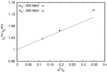
Particular drawbacks of this strategy are the significant cutoff effects which we ob- serve in the various definitions of t₀/a² on our largest lattice spacings, as discussed in

JHEP02(2015)043

section 7.1. Furthermore, the value of t₀ is not an experimentally accessible observ- able and only known from other lattice simulations. In the literature one finds √

8t0 = 0.4341(33) fm by the ALPHA collaboration using Wilson fermions in two-flavor QCD [28]

and √

8t₀ = 0.4144(59)(37) fm by the BMW collaboration using N_f =2+1 flavors [29]. In a 2 + 1 + 1 flavor setup with rooted staggered fermions, the HPQCD collaboration finds

√8t₀ = 0.4016(23) fm [30]. As has been observed in ref. [28], these numbers exhibit a sig- nificant flavor content effect, which however is monotonic in the number of flavors. Since our simulation setup is also withN_f = 2 + 1 flavors, we choose the value of ref. [29].

The QCD values of mπ = 134.8(3) MeV and mK = 494.2(4) MeV in the isospin limit and without electromagnetic contributions are taken from the analysis of ref. [31]. The correction of the experimental masses is based on ChPT at NLO with input from other lattice calculations showing a suppression of the contribution from the combination of low-energy constants relevant to this case. This leads to a physical point estimate

φ^phys₂ = 0.0801(27), φ^phys₄ = 1.117(38), (2.6) where errors have been added in quadrature.

From this choice and our measurements of t0/a² presented below, we estimate for our three values of β = 3.4, 3.55 and 3.7 lattice spacings a of a ≈ 0.086 fm, 0.064 fm and 0.05 fm, respectively.

2.3 Quark mass trajectory

In order to achieve O(a) improvement, the bare coupling — as all bare parameters — has to be improved with a mass-dependent term [24]

˜ g₀² =g²₀





 1 +bg

3aX

f

(m0,f−mcr)







, (2.7)

with mcr the critical quark mass whose precise value is not known at this stage. To keep the lattice spacing constant as we change the sea quark masses, this modified coupling constant ˜g0 has to be kept constant.

While the coefficientbg is small at one loop in perturbation theory [32],bg= 0.012Nfg²₀, a non-perturbative result is not known for any action. To keep ˜g0 fixed, we therefore keep the sum over the subtracted quark masses fixed, a strategy already proposed in ref. [14].

Note that this is equivalent to keeping the sum over the bare quark massesm0,f fixed a

3

X

f=1

(m_0,f−mcr) = const ⇔ a

3

X

f=1

m_0,f = const ⇔

3

X

f=1

1

κ_f = const. (2.8) Up to effects of order O(amud), this also implies a constant sum of improved PCAC quark masses [33].

We can therefore define chiral trajectories by a point in the φ2–φ4 plane, at which different lattice spacings are matched and the requirement that the sum of the bare quark

JHEP02(2015)043

masses is constant. For each value of β, the lattice spacing is constant along these lines and a continuum limit can be performed for each value of φ2.

As explained in the next section, we match lattices with different lattice spacings at m_π = m_K ≈ 420 MeV, where we will also show first results concerning the size of the O(am) cutoff effects introduced by this choice.

2.4 Tuning strategy

By choosing the chiral trajectories of eq. (2.8), the tuning process can be highly simplified:

keeping β fixed, for each chiral trajectory we match the lattices at the flavor symmetric point, i.e. where all quarks have equal masses.

Determining the slope of φ₄ as a function of φ₂ at β = 3.4 from a set of preliminary runs, not shown here, we estimate the target value on the symmetric line

φ4

mud=ms = 1.15. (2.9)

With the final statistics, we are able to reach better than 1% accuracy in this quantity and a matching of the target value within one standard deviation. In the chiral limit this translates into an accuracy of about 1 MeV in the strange-quark mass. In the future, we plan to have more chiral trajectories which will allow us to study the consequences of the remaining mistuning.

The result of the tuning effort and the resulting trajectory in the φ₂–φ₄ plane is shown in figure1 with results from the ensembles given in table 1. Within the statistical accuracy, we do not observe significant cutoff effects. The one point at β = 3.7 is still under production and its error therefore not yet trustworthy. We observe, the quark mass effect onφ4 along this trajectory is moderate, around 5% between the chiral limit and the symmetric point, as expected from ChPT.

3 Algorithmic parameters

The basic algorithmic setup has already been described in detail in ref. [12], but since we are presenting simulations with larger lattices, statistics and a different action, the various settings needed to be reconsidered. Here we give the parameters at which the runs were performed and the reasoning behind the various choices.

3.1 Twisted-mass reweighting

Since the Wilson Dirac operator is not protected against eigenvalues below the quark mass, field space is divided by surfaces of zero eigenvalues. These barriers of infinite action cannot be crossed during the molecular dynamics evolution, at least if the equations of motion are integrated exactly.

While at a sufficiently large volume and quark mass this might not be a problem in practice [34], it can lead to instabilities during the simulation and meta-stabilities in the thermalization phase. L¨uscher and Palombi [10] therefore suggested to introduce a small twisted-mass term into the action during the simulation and compensate for this by reweighting.

JHEP02(2015)043

1.04 1.06 1.08 1.1 1.12 1.14 1.16 1.18 1.2

0 0.1 0.2 0.3 0.4 0.5 0.6 0.7 0.8 φ4

φ₂

β=3.4 β=3.55 β=3.7 phys.point

Figure 1. Position of our ensembles in terms of the dimensionless variables φ2 and φ4 defined in eq. (2.5). The rightmost points are on the symmetric line m_ud =m_s. The fact that the point with the smallestφ2 atβ = 3.7 is above the range indicated by coarser lattices might be an effect of mistuning at the symmetric point or an indication for underestimated errors due to the low statistics indicated by the dashed error bars.

id β Ns Nt κu κs mπ[MeV] mK[MeV] mπL

B105 3.40 32 64 0.136970 0.13634079 280 460 3.9

H101 3.40 32 96 0.13675962 0.13675962 420 420 5.8

H102 3.40 32 96 0.136865 0.136549339 350 440 4.9

H105 3.40 32 96 0.136970 0.13634079 280 460 3.9

C101 3.40 48 96 0.137030 0.136222041 220 470 4.7

D100 3.40 64 128 0.137090 0.136103607 130 480 3.7

H200 3.55 32 96 0.137000 0.137000 420 420 4.4

N200 3.55 48 128 0.137140 0.13672086 280 460 4.4

D200 3.55 64 128 0.137200 0.136601748 200 480 4.2

N300 3.70 48 128 0.137000 0.137000 420 420 5.1

N301 3.70 48 128 0.137005 0.137005 410 410 4.9

J303 3.70 64 192 0.137123 0.1367546608 260 470 4.1

Table 1. List of the ensembles. In the id, the letter gives the geometry, the first digit the coupling and the final two label the quark mass combination. We give rounded values ofmπ andmK using the t₀/a² of the ensemble and √

8t₀ = 0.4144 fm. Using t₀/a² extrapolated to the physical light quark masses, we estimate lattice spacings ofa≈0.086 fm, 0.064 fm and 0.05 fm forβ = 3.4, 3.55 and 3.7, respectively.

JHEP02(2015)043

In the present simulations, we use the second version of the reweighting suggested in ref. [10], which is less affected by fluctuations in the reweighting factor from the ultraviolet part of the spectrum of the Dirac operator. Contrary to the original proposal, we do not apply it to the Hermitian Dirac operator Q = γ₅D_W but to the Schur complement Qˆ =Qee−QeoQ⁻¹_ooQoe of the asymmetric even-odd preconditioning [35]. This amounts to replacing the determinant of the light quark pair by

detQ² = det²Q_oo det ˆQ² →det²Q_oo det Qˆ²+µ²₀

Qˆ²+ 2µ²₀ det ˆQ²+µ²₀

. (3.1)

The reweighting factor which needs to be included in the measurement of primary observ- ables then reads

W₀ = det( ˆQ²+ 2µ²₀) ˆQ²

( ˆQ²+µ²₀)² . (3.2)

The choice of the parameterµ₀ will be discussed in section5.1.

3.2 Determinant factorization

The fluctuations in the forces have to be reduced further than what can be achieved by introducing an infrared cutoff by the twisted mass µ0. To this end we use Hasenbusch’s mass factorization [36] with a twisted mass [37] applied to the last term in eq. (3.1) [38]

det ˆQ²+µ²₀

= det ˆQ²+µ²_N

mf

×

N_mf

Y

i=1

det

Qˆ²+µ²_i−1

Qˆ²+µ²_i (3.3) with a tower of increasing values of µ₀ < µ₁ < · · · < µ_Nmf. The values of these masses can significantly influence the performance of the algorithm. Here we roughly set them at equal distances on a logarithmic scale as suggested in ref. [12]. The precise values of the µ_i are listed in table2, which implicitly gives also the number of factors in eq. (3.3).

The combination of twisted-mass reweighting and mass factorization leads to an effec- tive action for the light quark pair withN_mf + 2 terms

S_ud,eff[U, φ₀, . . . , φ_Nmf+1] = φ₀,Qˆ²+ 2µ²₀ Qˆ²+µ²₀ φ₀

! +

Nmf

X

i=1

φ_i, Qˆ²+µ²_i Qˆ²+µ²_i−1φ_i

!

+ (

φ_Nmf+1, 1 Qˆ²+µ²_N

mf

φ_Nmf+1

!

−2 log detQ_oo )

.

(3.4)

The single term with the largest twisted mass and the one from the diagonal determinant detQoo are always integrated together and are therefore counted as one term.

3.3 RHMC

The strange quark is simulated using the RHMC algorithm [39, 40], where the matrix square root is approximated by a rational function

detQ= detQ_oo det q

Qˆ² = detQ_oodet



A⁻¹

Np

Y

i=1

Qˆ²+ ¯µ²_i Qˆ²+ ¯ν_i²



×W₁. (3.5)

JHEP02(2015)043

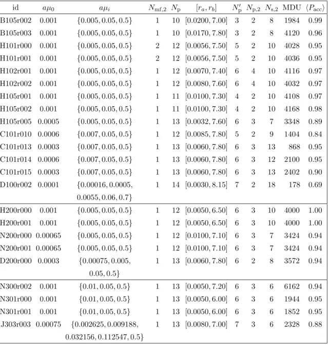
id aµ₀ aµ_i N_mf,2 N_p [r_a, r_b] N_p⁰ N_p,2 N_s,2 MDU hP_acci B105r002 0.001 {0.005,0.05,0.5} 1 10 [0.0200,7.00] 3 2 8 1984 0.99 B105r003 0.001 {0.005,0.05,0.5} 1 10 [0.0170,7.80] 3 2 8 4120 0.96 H101r000 0.001 {0.005,0.05,0.5} 2 12 [0.0056,7.50] 5 2 10 4028 0.95 H101r001 0.001 {0.005,0.05,0.5} 2 12 [0.0056,7.50] 5 2 10 4036 0.95 H102r001 0.001 {0.005,0.05,0.5} 1 12 [0.0070,7.40] 6 4 10 4116 0.97 H102r002 0.001 {0.005,0.05,0.5} 1 12 [0.0080,7.60] 6 4 10 4032 0.97 H105r001 0.001 {0.005,0.05,0.5} 1 11 [0.0100,7.30] 4 2 10 4108 0.97 H105r002 0.001 {0.005,0.05,0.5} 1 11 [0.0100,7.30] 4 2 10 4168 0.98 H105r005 0.0005 {0.005,0.05,0.5} 1 13 [0.0032,7.60] 6 3 7 3348 0.89 C101r010 0.0006 {0.007,0.05,0.5} 1 12 [0.0085,7.80] 5 2 9 1404 0.84 C101r013 0.0003 {0.007,0.05,0.5} 1 13 [0.0060,7.80] 6 3 13 868 0.95 C101r014 0.0006 {0.007,0.05,0.5} 1 13 [0.0060,7.80] 6 3 12 2100 0.95 C101r015 0.0003 {0.007,0.05,0.5} 1 13 [0.0060,7.80] 6 3 13 2402 0.90 D100r002 0.0001 {0.00016,0.0005, 1 14 [0.0030,8.15] 7 2 18 178 0.69

0.0055,0.06,0.7}

H200r000 0.001 {0.005,0.05,0.5} 1 12 [0.0050,6.50] 6 3 10 4000 1.00 H200r001 0.001 {0.005,0.05,0.5} 1 12 [0.0050,6.50] 6 3 10 4000 1.00 N200r000 0.00065 {0.005,0.05,0.5} 1 12 [0.0100,7.10] 6 3 7 3424 0.94 N200r001 0.00065 {0.005,0.05,0.5} 1 12 [0.0100,7.10] 6 3 7 3424 0.94 D200r000 0.0003 {0.00075,0.005, 1 13 [0.0060,7.80] 6 2 8 3572 0.94

0.05,0.5}

N300r002 0.001 {0.01,0.05,0.5} 1 13 [0.0050,7.20] 6 3 6 6162 0.94 N301r000 0.001 {0.01,0.05,0.5} 1 13 [0.0050,6.00] 6 3 6 1944 0.95 N301r001 0.001 {0.01,0.05,0.5} 1 13 [0.0050,6.00] 6 3 6 1852 0.95 J303r003 0.00075 {0.002625,0.009188, 1 13 [0.0080,7.00] 7 3 6 2328 0.88

0.032156,0.112547,0.5}

Table 2. Parameters of the algorithm: we give the twisted masses used in the reweighting and mass factorization, theNmf,2lightest of which are integrated on the coarsest time scale, the number of polesN_pand the range used in the RHMC, withN_p⁰ put on single pseudofermions ,N_p,2of which are integrated on the outer level. Ns,2is the number of steps of the outer level of the MD integrator used for one trajectory. The total length of the Markov chain and the acceptance rate are also given.

JHEP02(2015)043

Zolotarev’s optimal approximation to the inverse square root in the interval [r_a, r_b] with a given number of poles Np determines the parameters A and {¯µi,ν¯i}. The strange-quark mass as argument of Qand ˆQ has been suppressed for readability. W₁ is the reweighting factor, implicitly defined by eq. (3.5), which has to be included in the measurement. The values used in the various runs are specified in table2.

The openQCD code gives the option to split the determinant of the rational function in eq. (3.5) into several factors. In our simulations, we represent the N_p⁰ terms with the smallest ¯µi of the product eq. (3.5) by single pseudofermions, whereas the determinant of the remaining factors is expressed as a single pseudofermion integral

S_s,eff[U, φ₀, . . . , φ_Np⁰] =

N_p⁰−1

X

i=0

φ_i,

Qˆ²+ ¯ν_N²_p−i Qˆ²+ ¯µ²_N

p−i

φ_i

! +



φ_Np⁰,

Np−N_p⁰

Y

j=1

Qˆ²+ ¯ν_j² Qˆ²+ ¯µ²_jφ_Np⁰





−log detQ_oo.

(3.6)

Here again, the contribution from the two final terms is always considered together.

This decomposition has several advantages. First of all, the small residues frequently can be integrated on a larger time scale, due to a small coefficient decreasing the forces.

Furthermore, while the multi-shift conjugate gradient algorithm [41] is efficient for the combined solution of the systems in the last factor with the large shifts, it turns out to be advantageous to employ the deflated solver for the terms involving the smaller ¯µ_i. In this case it is no longer necessary to use a single pseudofermion field for all shifts.

The range of the rational approximation is given by the smallest and the largest eigen- value of ˆQ² over typical gauge field configurations. On thermalized configurations, esti- mates of these numbers can be obtained in openQCD by the power method applied to ˆQ⁻² and ˆQ², respectively. Typically, O(20) iterations proved sufficient for the lower bound, whereas the largest eigenvalue required O(100) iterations. In particular the smallest eigen- value turned out to be sensitive to thermalization effects and exhibit larger fluctuations than expected. This made it necessary to monitor it carefully at the beginning of each production run.

3.4 HMC and the integration of the molecular dynamics

In the algorithm the action is split into different components: the gauge action, the de- terminants from the Hasenbusch splitting for the light quarks and the various contribu- tions to the strange-quark determinant from the rational approximation described above, N_mf+N_p⁰+4 components in total. The complete action is simulated with the Hybrid Monte Carlo (HMC) algorithm [42]; the classical equations of motion are solved numerically for trajectories of length τ = 2 in all simulations. This leads to Metropolis proposals which are accepted with an acceptance ratehP_acci, given for our runs in table2.

The goal of the splitting of the action, and the forces deriving from it, is the reduction of the computational cost needed to obtain a high acceptance rate at the end of the trajectory.

The gauge forces are much cheaper to compute than the fermion forces, whose components differ by orders of magnitude in size and fluctuations. It is therefore natural to use a hierarchical integration scheme for the molecular dynamics of the HMC to reflect this [43].

JHEP02(2015)043

We use the setup described in ref. [12], i.e., a three-level scheme with the gauge fields integrated on the innermost level with the fourth order integrator suggested by Omelyan, Mryglod, and Folk (OMF) [44] and implemented in the openQCD code. Most of the fermion forces are on the intermediate level, again integrated with the fourth order integration scheme. Only particularly small components of the fermion forces, that contribute little to energy violation, are integrated on a larger scale with the second order OMF integrator [44], whose parameter λis set to 1/6.

Since one step of an inner level integration scheme is done for each outer step, there are three parameters which define the scheme: the number of outermost steps per trajectory Ns,2 and the number of poles Np,2 as well as the number Nmf,2 of terms of eq. (3.3) integrated on the outermost level. In the latter two cases the numbers refer to the terms with the smallest twisted-mass shifts. The values chosen in our runs can be found in table2.

The choice of the trajectory length affects the autocorrelation times and is therefore not easily studied. In general, longer trajectories have proven to be beneficial [4], but in particular with dynamical fermions one might prefer shorter trajectories because of instabilities of the integrator. As a compromise, we use τ = 2. Asymptotically, this leads to autocorrelations growing with τ_int ∝a⁻². Note, however, that this scaling behavior is also expected if the length of the trajectory is scaled [45].

3.5 Solver

The extensive use of the locally deflated solver [46–48] is an important part of the progress that made the presented simulations possible. It removes the largest part of the cost increase as the quark mass is lowered, thereby circumventing the significant slowing down observed in the past. The increase in performance of the solver comes at the price of a more complex setup and many additional parameters which have to be chosen.

Fortunately, relatively little tuning of the local deflation subspace was necessary here and we therefore do not list the parameters in detail. For most runs, we used deflation blocks of size 4⁴. The parallelization of theN_s = 48 lattices required one or two dimensions to be set to 6; also blocks of 8×4³ have been used.

The number of deflation modes per block has been chosen between 20 and 32, in order to balance the higher efficiency provided by the larger subspace and the cost associated with the application of the preconditioner.

For the smaller lattices with L/a= 32, we set the solver accuracy (the ratio between the norm of the residue to the norm of the right hand side of the equation) to 10⁻¹¹ in the action and 10⁻¹⁰ in the force computation. To ensure the value of the action and the reversibility of the integration of the equations of motion are sufficiently precise, more stringent residues have been used for the lattices of larger volume.

3.6 Production cost

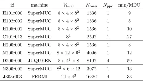
To give an idea of the cost of the various ensembles, we show in table 3the average wall- clock time per molecular dynamics unit, along with the machine on which the run has been performed, the local lattice geometry, and the total number of cores used. Most of our production runs were carried out either on SuperMUC, a petascale cluster of IBM

JHEP02(2015)043

id machine V_local N_cores N_ppc min/MDU

H101r000 SuperMUC 8×4×8² 1536 1 9

H102r002 SuperMUC 8×4×8² 1536 1 8

H105r002 SuperMUC 8×4×8² 1536 1 10

C101r013 SuperMUC 8⁴ 2592 1 27

H200r000 SuperMUC 8×4×8² 1536 1 8

N200r000 SuperMUC 8×12×6² 4096 1 12

D200r000 JUQUEEN 8×4²×8 8192 4 59

N300r002 SuperMUC 8²×6×12 3072 1 13

J303r003 FERMI 12×4³ 16384 4 33

Table 3. Production setup of selected runs. The last column shows the wall-clock time in minutes per molecular dynamics unit on the specific machines used in this project. The other columns give the local lattice size per MPI process (V_local), the number of cores used (N_cores), and the number of MPI processes run on each core (N_ppc). Since execution times also depend on the actual system software and on the run-time environment, the last column can provide only a rough indication of the cost of the simulations.

System x iDataPlex servers with Intel Sandy Bridge-EP processors (Xeon E5-2680 8C) and Infiniband network (FDR10), or on IBM BlueGene/Q systems at CINECA (FERMI) and JSC (JUQUEEN). Since our code is not multi-threaded, we launch four MPI processes per core on the BlueGene/Q machines to maximize overall performance.

Note that the execution times of the simulations do not only depend on the algorithmic parameters (even for a single specific trajectory), but also on the particular hardware on which the code has been run, as well as on the system software (e.g. compiler and library versions) and on the run-time environment. The latter may — and usually do — change during the months of production. Therefore, the times quoted here can only serve as an indication of the approximate cost of the simulations and have to be taken with care.

4 Autocorrelations

Markov Chain Monte Carlo algorithms, like the Hybrid Monte Carlo used here, produce field configurations which exhibit autocorrelations characterized for an observableAby the autocorrelation function

Γ_A(t) =hA_tA₀i − hAi², (4.1)

wheretis the Monte Carlo time. The integral over the normalized autocorrelation function ρ(t) enters the error analysis. This is the integrated autocorrelation time

τint(A) = 1 2 +

∞

X

t=1

ρA(t)≡ 1 2+

∞

X

t=1

Γ_A(t)

ΓA(0). (4.2)

To estimateτint(A) with a finite variance, it is necessary to cut the summation at a window W [50,51]. In order to choose the window for our final error estimates and to account for

JHEP02(2015)043

0 20 40 60 80 100 120 140 160

0 1 2 3 4 5 6 7 8 9 10 11 12 τint / MDU

t₀/a²

E(t₀) Q²(t₀)

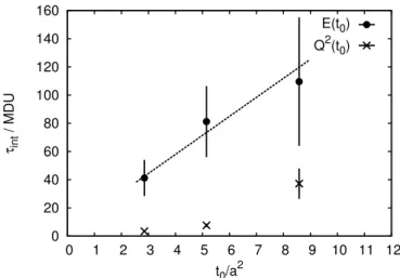
Figure 2. Scaling of the integrated autocorrelation time of Q²(t0) andE(t0). For the energy, we observe very good scaling, whereas for the charge, significant violations are observed. At coarser lat- tices the topological charge decorrelates significantly faster than predicted by the scaling hypothesis, very similar to the pure gauge case [7].

the thereby neglected tail, we employ the method described in ref. [4]. Its essential input is an estimate for the exponential autocorrelation time, which we discuss in the following.

4.1 Scaling of the autocorrelations

As we approach the continuum limit, the autocorrelation times are expected to grow due to critical slowing down. The open boundary conditions used in our setup should prevent catastrophic scaling due to the freezing of the topological charge. Since we have chosen the trajectory length constant in all our runs, we expect Langevin scaling τ_int∝a⁻².

In figure 2 we show autocorrelation times of notoriously slow observables: the global topological charge and the action density averaged over the plateau region, both con- structed from links smoothed by the Wilson flow integrated to flow timet₀. They are both defined in eq. (6.2). We find a situation similar to that encountered in pure gauge theory [7].

While the energy density shows very good scaling, the topological charge decorrelates faster on coarser lattices.

The fast growth of the integrated autocorrelation time of the charge does not mean that the 1/a² scaling is not valid. In pure gauge theory, the behavior could very well be fitted with τint ∝ a⁻²(c+da²). In this picture, there are significant cutoff effects to the scaling, but no catastrophic behavior in thea→0 limit. This is expected when simulating with open boundary conditions.

4.2 Cost of the simulation

Note, in two-flavor QCD with periodic boundary conditions at a lattice spacing of roughly a = 0.05 fm [8] the topological charge does not decorrelate slower than the smoothed energy. Rather, it shows similar autocorrelations for quark masses around 400 MeV. This means that we are not yet in the position to fully profit from the effect of the open boundary

JHEP02(2015)043

conditions, however, going to finer lattice spacings the freezing observed in two-flavor QCD ata≈0.03 fm [52] will be avoided.

In the sense of fast decorrelations and minimal requirements on the number of units of molecular dynamics time (MDU), the presented simulations are not cheap, nevertheless.

The exponential autocorrelation time ofτexp ≈14(3)t0/a² is consistent with what is found in figure 2. For biases to be small and a simulation to be reliable we need a total Monte- Carlo history of at least O(50)×τexp. Forβ= 3.4 this translates to 2000 MDU, whereas for β = 3.55 and β = 3.7 a statistics of 3600 MDU and 6000 MDU, respectively, is necessary.

For most of our ensembles listed in table1, we exceed these numbers, but for some, which are still in production, they are not yet reached. Those quoted results therefore have to be taken with care in these cases.

5 Reweighting factors

The simulations are not done with the exact QCD action as given by eqs. (2.1) and (2.3), but differ due to the twisted-mass reweighting eq. (3.4) and the inaccurate rational function in the RHMC eq. (3.6). The observables are reweighted to the target theory, for which the reweighting factorW =W0W1 needs to be computed. The factors W0 andW1, as defined in eqs. (3.2) and (3.5) respectively, contain ratios of determinants which are estimated stochastically as described below.

Expectation values hAi of primary observablesA can then be computed from expec- tation values in the theory with the modified actionh· · · i_W, according to

hAi= hAWi_W

hWi_W . (5.1)

5.1 Twisted-mass reweighting factor

The twisted-mass reweighting plays an important role in our setup. From a conceptual point of view, it removes barriers of infinite action created by zero eigenvalues of the Wilson Dirac operator. Together with Hasenbusch factorization, it also reduces the fluctuations of the forces which makes the simulations cheaper and more reliable in practice [38].

This situation is especially favoured for a large value of µ₀ in eq. (3.2). It might, however, also lead to significant fluctuations in the reweighting factor and as a consequence to a larger statistical error of certain observables.

As a consequence, what constitutes the optimal choice of the parameter µ₀ will in general depend on the observable. As can be seen in figure 3, W₀ is close to a constant for most configurations; only on some configurations the value will be much smaller. For observables with little or no correlation to the reweighting factor, like the gluonic ones we consider below, this effectively amounts to a reduction in statistics [53]. This reduction is negligible for our ensembles sincehvar(W)i hWi² in all cases.

For observables with a strong correlation withW₀, the situation is more delicate. Even after reweighting, this can lead to large fluctuations in the measurements and significantly increased statistical error. In particular in the case of anticorrelation, the situation is more problematic due to the stochastic estimation of W and, possibly, the observable. The

JHEP02(2015)043

0 0.2 0.4 0.6 0.8 1 1.2

W/<W>

aµ₀=3 ⋅10^-4 aµ₀=6 ⋅10^-4

0 0.2 0.4 0.6 0.8 1 1.2

10 30 100 300 1000

fPP⋅106

10 30 100 300 1000

1 3 10 30 100

0 1000 2000

W/<W> fPP⋅106

MDU

1 3 10 30 100

0 1000 2000

MDU

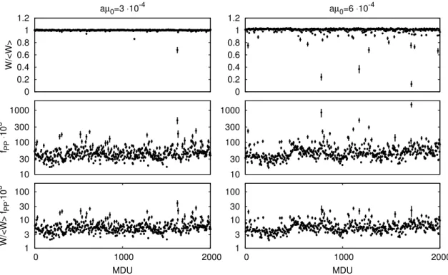
Figure 3. Time history of the reweighting factor (top), the pseudoscalar correlatorf_PP(x₀) (center) and the productW fPP(x0) (bottom) on two C101 ensembles with different values of the reweighting parameter,aµ0 = 0.0003 andaµ0 = 0.0006, respectively, evaluated on time-slice x0 = (T +a)/2.

The error bars indicate the uncertainty due to the stochastic estimation of these quantities.

cancellation between, e.g. a large value of the observable and a small value of W might require a rather precise determination of the two.

5.2 Reweighting and the pseudoscalar correlation function

The pseudoscalar correlation function is an observable showing a strong anticorrelation between its value and the reweighting factor. This can be easily understood by noting that at small quark masses both receive significant contributions from the smallest (in magnitude) eigenmodes of the Hermitian Dirac operator. It is precisely this region where the reweighting term has the largest effect.

To illustrate the cancellation between the fluctuations in W and f_PP(x₀), figure 3 displays the time series of the two (top and central panel) atx0 = (T+a)/2 together with the productW f_PP(x₀); see eq. (6.7) for its definition. Data for C101 and two values of µ₀ is shown. As we can see, the larger µ₀ leads to larger fluctuations in W and f_PP(x₀), as expected. In the product, however, they cancel and the average valuehW f_PP(x0)i/hWi is then consistent within the statistical errors between the two ensembles.

5.3 Computation of W₀

Since the determinant ratios needed for the computation of W0(µ0) cannot be computed directly, a stochastic estimator is taken instead. This can either be done by directly esti- mating the determinant ratio in eq. (3.2) or by first splitting it up and then using stochastic

JHEP02(2015)043

estimates for the individual factors [54], a strategy already successful in Hasenbusch’s mass factorization.

Among the many possibilities, we here restrict ourselves to splitting the interval be- tweenµ= 0 and µ=µ₀ intoN_sp smaller steps µ₀= ˜µ₀ >µ˜₁ >· · ·>µ˜_Nsp = 0

W₀(µ₀) =

Nsp

Y

i=1

detR(˜µi−1,µ˜_i) ; R(µ₁, µ₂) = ( ˆQ²+µ²₂)² ( ˆQ²+µ²₁)²

( ˆQ²+ 2µ²₁)

( ˆQ²+ 2µ²₂). (5.2) Now each of the factors is evaluated stochastically withN_r complex-valued Gaussian ran- dom fieldsη of unit variance

R(µ˜ ₁, µ₂, N_r) = 1 Nr

Nr

X

i=1

exp{− η_i,(R⁻¹(µ₁, µ₂)−1)η_i

}, (5.3)

such that up to an irrelevant constant factor the determinant is retrieved by averaging over the noise fields

detR(µ1, µ2)∝ hR(µ˜ 1, µ2, Nr)i_η. (5.4) Following the initial proposal of ref. [12], it is sufficient to use a single stepN_sp = 1 with a suitably chosen value ofN_r. Its value along with the other parameters of the reweighting can be found in table4. This is the method implemented in openQCD-1.2.

Once the fluctuations in the reweighting factor increase, it is advisable to use interme- diate ˜µ, a possibility given in openQCD-1.4. This is because the distribution of the results for the reweighting factors become long-tailed once exceptionally small eigenvalues of the Qˆ² are encountered. In this situation it is very difficult to argue about the uncertainty of W0 [55]. By splitting the estimate into smaller intervals in ˜µ, the distribution of each of the factors becomes significantly more regular.

For ensemble H105r002 we find precisely such a situation. While with a single step in

˜

µ the smallest reweighting factors show a distribution which is far from Gaussian, using ten intermediate ˜µ the individual factors can be computed reliably to O(15%) accuracy using 15 sources each.

5.4 RHMC reweighting factor

Since the rational approximation has been chosen to a good accuracy, the fluctuations in the reweighting factor are small and it turns out to be sufficient to estimate it with one stochastic source per configuration. The associated variances are given in table 4. They are seen to receive a considerable contribution from the stochastic estimation of W₁.

In order to study the effect of more sources, we observe using five instead of one stochastic estimate reduces the variance of W₁ by more than a factor 4, on ensemble H105r005. The same is true for the H200 ensembles. Still, even with one source per gauge configuration the noise introduced by W1 is negligible for all observables we investigated.

Note that in some early runs we underestimated the upper bound of the interval in which the rational function is accurate. Since the accuracy does not deteriorate quickly outside the interval, the fluctuations of the reweighting factors nevertheless are suffi- ciently small.

JHEP02(2015)043

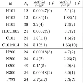
id N_r ^var(W_hW ⁰⁾

0i² ·10^{3 var(W}_hW ¹⁾

1i² ·10⁵ H101 12 0.00047(9) 5.1(2)

H102 12 0.036(4) 1.88(5)

H105 36 3.2(4) 7.3(2)

H105r005 24 0.0032(9) 3.7(2)

C101 24 1.8(1.1) 1.6(2)

C101r014 24 5.1(2.1) 1.63(10) H200 24 0.00018(5) 4.7(2)

N200 24 0.4(2) 2.23(7)

D200 48 0.15(5) 4.9(3)

N300 24 0.00018(2) 3.0(1)

J303 24 3.7(3.2) 1.3(2)

Table 4. Parameters of the reweighting. We give the number of sources Nr used to estimate the twisted-mass reweighting factor W₀ — for the RHMC reweighting factor W₁ we always use one source — and the resulting variances of W0 and W1. Nsp = 1 in all cases. H105 refers to runs r001 and r002, whereas C101 to runs r013 and r015. J303 have not reached sufficient statistics for a reliable result.

6 Observables

6.1 Wilson flow

The Wilson flow can be a very useful tool in lattice QCD from which quantities with a finite continuum limit can be constructed [6,56,57]. The gauge fields U(x, µ) are subjected to the smoothing flow equation

∂_tV_t(x, µ) =−g²₀{∂_x,µS_W(V_t)}V_t(x, µ), V_t(x, µ)

t=0= U(x, µ), (6.1) with S_W being the Wilson action. With clover-type discretization of the field strength tensor ˆGµν(x, t) constructed from the smooth fieldsVt, the time slice energy E(x0, t) and the global topological chargeQ_top(t) can be constructed

E(x0, t) =− a³ 2L³

X

~ x

tr{Gˆµν(x, t) ˆGµν(x, t)}, Qtop(t) =− a⁴

32π² X

x

µναβtr{Gˆµν(x, t) ˆGαβ(x, t)}.

(6.2)

With the vacuum expectation value of the energyhE(t)i, the scale parametert₀ is then defined by

t²E(t)

t=t0 = 0.3. (6.3)

Throughout this paper we quote the observables of eq. (6.2) at flow timet₀.

JHEP02(2015)043

0.2 0.4 0.6 0.8 1

0 2 4 6 8 10 12 14 16

t02 E(x0,t0)

x₀/√t₀

β=3.4 β=3.55 β=3.7

Figure 4. In the vicinity of the boundary, significant cutoff effects inE(x₀, t₀) are observed. They are noticable in the expected region: x0 = 4ais roughly at x0/√

t0 = 2.3, 1.7 and 1.4 forβ= 3.4, 3.55 and 3.7, respectively. At the same time, the dependence on the quark masses is negligible:

for each lattice spacing we plot the data for all available quark masses. The dotted lines represent fits to eq. (6.4). They are used to set the lower bound of the plateau fit indicated by the vertical dashed line.

6.2 Effects of the boundary

Due to the open boundary conditions in the temporal direction, time translational invari- ance is lost. Sufficiently far away from the boundaries, local observables are expected to assume their vacuum expectation values up to exponentially small corrections with a decay rate equal to the lightest excitation with vacuum quantum numbers.

On top of this continuum boundary effect, large discretization errors are observed close to the boundary. As an example we show in figure 4the behavior of the smoothed energy E(t, x0), defined in eq. (6.2). A further example for the pseudoscalar correlation function with the sink approaching the boundary can be found in ref. [53].

In the case of the energy, it should be noted that it is at this point difficult to disentangle the discretization effects in the underlying gauge field from the ones introduced by the Wilson flow and the observable used to define the field strength tensor, but recent work by Ramos and Sint might clarify this issue [58]. Also the Dirac operator used in the measurement of the effective mass is only tree-level improved at the boundary. Still, the effects of the finite lattice spacing are very prominent at our coarser lattices, but become much less notable as the continuum limit is approached.

As can be seen in figure 4, no sizable dependence on the quark mass is observed in t²₀E(x₀, t₀). This is trivial for the bulk, since its value is equal to 0.3 by definition. But also the (cutoff) effects close to the boundaries show no quark mass dependence. Whether this is a generic feature of the sea quark contribution being small or it is due to our particular choice of chiral trajectory eq. (2.8) cannot be judged from the data presented here.

In the context of the present paper we will not discuss these effects in detail, but perform the measurements in a region where they can be neglected. The determination

JHEP02(2015)043

of the plateau region is not always clear due to an effect already observed in ref. [12]:

in precise observables, like the examples above, long-range waves are visible. They are a consequence of the limited statistics and do not exceed what is expected if the statistical analysis is done properly, however, they do make the plateau determination more difficult.

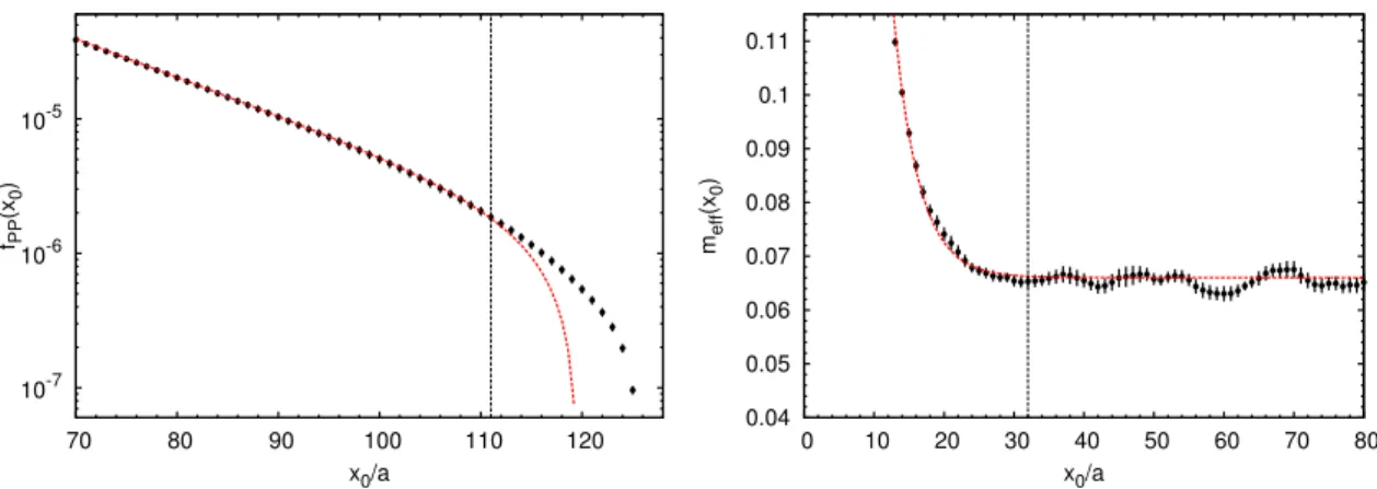
For meson correlation functions, these waves have been discussed previously [59], see figure 6 for an example from our simulations. In other simulations they are typically not visible, because time translational invariance is used on the level of the correlation function by using different source positions in time and averaging them before computing effective masses. Again, this is not a principal problem. However, we need to ensure sufficient statistics and that errors are under control and require a procedure to deal with these waves.

6.3 Measurement of t₀

For the determination oft0, we need to determine the plateau inE(x0, t) for t=t0. Since we are looking at a smoothing radius of√

8t₀, the effects of the boundary visible in figure4 are at the expected length scale. Discretization effects are large though, and it is therefore difficult to argue about the expected functional form. In this situation, we use a two-stage procedure: first we fit

E(x0, t) =E(t) +c0e^−mT2 cosh

−m

x0−T 2

(6.4) in the range where this ansatz describes the data. This is only used to determine the fit range by the condition that in the whole range the statistical uncertainty δE(x0) is dominating over the systematic effect from a non-vanishing c₀, i.e., we require for the fit interval [x_0,min, T −x_0,min]

1

4δE(x0,min, t)> c0e^−mT2 cosh

−m

x0,min−T 2

. (6.5)

At the current accuracy of the data, the result of this investigation is that a singlex_0,min is sufficient for each value of β, as might be expected from figure4. The effect of the quark mass is negligible. In particular we have

x0,min(β = 3.4)/a= 20 ; x0,min(β= 3.55)/a= 21 ; x0,min(β = 3.7)/a= 24, (6.6) and the final value of E(t) in the vicinity of t=t₀ is determined by averaging E(x₀, t) in the corresponding interval. The value oft0/a² is then determined by eq. (6.3). The results are listed in table5.

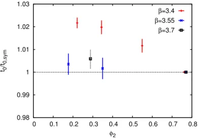
In figure 5 the quark mass dependence of t0 is given for the three available lattice spacings. Recall, the values are given in terms of the symmetric point which defines the chiral trajectory at m_ud = m_s. From a Taylor expansion around this point [14] as well as ChPT [27] one expects a constant behavior to the respective leading order. This is confirmed for the finer lattices to our level of accuracy. Only at the coarsest lattice spacing, cutoff effects seem to cause some deviation, albeit on a rather small scale.

JHEP02(2015)043

0.98 0.99 1 1.01 1.02 1.03

0 0.1 0.2 0.3 0.4 0.5 0.6 0.7 0.8 t0/t0,sym

φ₂

β=3.4 β=3.55 β=3.7

Figure 5. Dependence of t0/t0,sym on φ2, where t0,sym is the value at mud = ms along our trajectory. The dashed errorbars indicate the low statistics in the J303 ensemble.

6.4 Pseudoscalar masses

The masses of the pseudoscalar particles are computed from the pseudoscalar correlation function projected to zero momentum. With quark fields of flavor r and s, and the pseu- doscalar densityP^rs= ¯ψ^rγ₅ψ^s, it is given by

f_PP(x0, y0) =−a⁶ L³

X

~x,~y

hP^rs(x)P^sr(y)i . (6.7)

Due to the open boundary conditions in time, the translational invariance in the temporal direction is broken. However, we find that there is little to gain from using source fields at different time slices [53]. The U(1) stochastic source fields are therefore put only aty₀ =a and y₀=T−a[60]. In the following we analyze

f_PP(x0)≡ 1

2{f_PP(x0+a, a) +f_PP(T−a−x0, T−a)}. (6.8) In the continuum limit and for large volume and sink positions far away from the source and boundary, x0 0 and x0 T, the two-point function is expected to fall off as [12]

f_PP(x₀) =Asinh(m_PS( ˜T −x₀)). (6.9) In line with ref. [12], ˜T is a free parameter. We follow a similar strategy as in section 6.3 to make sure that in our final fit the excited state contribution is negligible.

We show an example of an effective mass plot in figure 6, where we can see that this fit works very well in a wide range of x0. The results for the masses are listed in table 5.

Even though we do not give results on decay constants, let us remark that also in this case the sources can be put in the vicinity of the boundaries. Methods similar to the ones already developed in the Schr¨odinger Functional [61] can be used to cancel the matrix element of the source operator such that only the sink has to be sufficiently far away