Characterizing cosmic neutrino sources

A Measurement of the Energy Spectrum and Flavor Composition of the Cosmic Neutrino Flux Observed with the IceCube Neutrino Observatory

DISSERTATION

zur Erlangung des akademischen Grades doctor rerum naturalium

(Dr. rer. nat.) im Fach Physik eingereicht an der

Mathematisch-Naturwissenschaftlichen Fakult¨at der Humboldt-Universit¨at zu Berlin

von

Lars Bastian Mohrmann

Pr¨asident der Humboldt-Universit¨at zu Berlin:

Prof. Dr. Jan-Hendrik Olbertz

Dekan der Mathematisch-Naturwissenschaftlichen Fakult¨at:

Prof. Dr. Elmar Kulke Gutachter:

1. Prof. Dr. Marek Kowalski 2. Prof. Dr. Klas Hultqvist

3. Priv.-Doz. Dr. Alexander Kappes Tag der m¨undlichen Pr¨ufung: 11.11.2015

The IceCube Neutrino Observatory is a km³-sized neutrino telescope located at the geographical South Pole. The telescope consists of an array of more than 5,000 photosensors, embedded deep in the glacial ice, that record the Cherenkov radiation emitted by secondary parti- cles created in neutrino interactions. Its primary purpose is the detec- tion of high-energy cosmic neutrinos. Such neutrinos are expected to be produced in interactions of high-energy cosmic rays with ambient matter or photons close to their acceleration sites. With their unique properties, neutrinos may help to identify these sites, and probe the acceleration process.

In 2013, the IceCube Collaboration has reported the first evidence for a flux of high-energy cosmic neutrinos. While the origin of the flux remains unknown so far, the properties of its sources can be constrained by measuring its energy spectrum and its composition of electron, muon, and tau neutrinos (designated as “flavor composition”). The present work constitutes the first comprehensive analysis of IceCube data with respect to these principal characteristics of the flux.

Several data sets that were originally collected for separate studies were assembled and simultaneously studied in a combined analysis.

Experimentally observed distributions of reconstructed energy, zenith angle and particle signature were fitted with model distributions for the background of atmospheric muons and neutrinos and for the cosmic neutrino flux. The combination of models that describes the data best was determined with a maximum-likelihood estimator.

Assuming the cosmic neutrino flux to be isotropic and to consist of equal flavors at Earth, the all-flavor spectrum is well described by a power law with normalization (6.7^+1.1_−1.2)×10⁻¹⁸GeV⁻¹s⁻¹sr⁻¹cm⁻² at 100 TeV and spectral index −2.50±0.09 for neutrino energies be- tween 25 TeV and 2.8 PeV. A spectral index of −2, an often-quoted benchmark value, is disfavored with a significance of 3.8 standard de- viations.

The flavor composition is compatible with that expected for standard neutrino production processes at the sources. However, a scenario in which only electron neutrinos are produced, e.g. in the decay of

the neutrino flavors during propagation from the sources to the Earth, the measured fraction of electron neutrinos at Earth is (18±11)%.

These results constitute the most precise characterization of the cos- mic neutrino flux observed with the IceCube Neutrino Observatory obtained so far.

Keywords:

Astroparticle physics, Neutrino, IceCube, Spectrum, Flavor

Das IceCube Neutrino Observatorium ist ein km³-großes Neutrino- teleskop und befindet sich am geographischen S¨udpol. Das Teleskop besteht aus mehr als 5.000 Photosensoren, die tief in das Gletschereis eingelassen sind und Cherenkov-Strahlung messen, welche von in Neu- trinowechselwirkungen erzeugten Sekund¨arteilchen abgestrahlt wird.

Das Hauptziel des Experiments ist es, hochenergetische kosmische Neu- trinos nachzuweisen. Es wird erwartet, dass solche Neutrinos in Wech- selwirkungen von hochenergetischer kosmischer Strahlung mit Materie oder Photonen in der N¨ahe ihrer Beschleunigungsumgebung entstehen.

Durch ihre einzigartigen Eigenschaften k¨onnen Neutrinos dazu beitra- gen, diese Umgebungen zu identifizieren und den Beschleunigungspro- zess zu untersuchen.

Der erste Nachweis f¨ur einen Fluss von hochenergetischen kosmi- schen Neutrinos wurde 2013 von der IceCube-Kollaboration erbracht.

Der Ursprung des Flusses ist noch nicht bekannt, dennoch k¨onnen die Eigenschaften der Quellen durch eine Messung des Energiespektrums und der Zusammensetzung aus Elektron-, Muon-, und Tau-Neutrinos (der “Flavor-Zusammensetzung”) des Flusses eingeschr¨ankt werden.

Die vorliegende Arbeit stellt die erste umfassende Analyse von Daten des IceCube-Experiments im Hinblick auf diese wesentlichen Eigen- schaften des Flusses dar.

Mehrere Datens¨atze, welche urspr¨unglich f¨ur separate Studien aus- gew¨ahlt wurden, wurden kombiniert und gemeinsam analysiert. Da- bei wurden experimentell beobachtete Verteilungen von rekonstruier- ter Energie, Zenithwinkel und Teilchen-Signatur mit Modellverteilun- gen f¨ur den Untergrund von atmosph¨arischen Muonen und Neutrinos und f¨ur den kosmischen Neutrinofluss angepasst. Die Kombination aus Modellen, welche die Daten am besten beschreibt, wurde mit einem Maximum-Likelihood-Sch¨atzer bestimmt.

Unter der Annahme, dass der Fluss isotrop ist und zu gleichen Teilen aus allen Neutrino-Flavors besteht, wird das Spektrum durch ein Po- tenzgesetz mit Normalisierung (6.7^+1.1_−1.2)×10⁻¹⁸GeV⁻¹s⁻¹sr⁻¹cm⁻² bei 100 TeV und spektralem Index −2.50±0.09 zwischen Neutrino- Energien von 25 TeV und 2.8 PeV gut beschrieben. Ein spektraler Index

Die Flavor-Zusammensetzung ist kompatibel mit Erwartungen f¨ur Standard-Prozesse der Neutrino-Produktion an den Quellen. Die aus- schließliche Produktion von Elektron-Neutrinos, z.B. durch den Zerfall hochenergetischer Neutronen, kann hingegen mit einer Signifikanz von 3.6 Standardabweichungen ausgeschlossen werden. Unter der Annah- me, dass die Neutrino-Flavor w¨ahrend der Propagation von den Quel- len zur Erde durch Standard-Neutrino-Oszillationen transformiert wer- den, betr¨agt der gemessene Anteil an Elektron-Neutrinos an der Erde (18±11)%.

Diese Ergebnisse stellen die bisher pr¨aziseste Charakterisierung des kosmischen Neutrinoflusses am IceCube Neutrino Observatorium dar.

Schlagw¨orter:

Astroteilchenphysik, Neutrino, IceCube, Spektrum, Flavor

1 Introduction 1 2 The Neutrino as a Messenger Particle 5

2.1 Fundamental Properties of Neutrinos . . . 8

2.1.1 Neutrino Production Processes . . . 10

2.1.2 Neutrino Interactions at High Energies. . . 11

2.1.3 Neutrino Oscillations. . . 13

2.2 Established Neutrino Sources . . . 16

2.2.1 Artificially Produced Neutrinos . . . 16

2.2.2 Neutrinos from the Supernova Explosion SN 1987a 18 2.2.3 Solar Neutrinos . . . 20

2.2.4 Atmospheric Neutrinos. . . 22

2.3 Predicted Neutrino Sources . . . 23

2.3.1 The Cosmic Neutrino Background . . . 24

2.3.2 The Diffuse Supernova Neutrino Background . . 24

2.3.3 Neutrinos from Dark Matter Annihilation or Decay 24 3 Neutrinos from the Acceleration Sites of Cosmic Rays 27 3.1 General Considerations. . . 29

3.1.1 Production Mechanisms . . . 29

3.1.2 Energy Spectrum . . . 31

3.1.3 Flavor Composition . . . 36

3.1.4 Connection to Ultra-High-Energy Cosmic Rays . 39 3.1.5 Connection to High-Energy Gamma Rays . . . . 41

3.2 Candidate Source Classes . . . 41

3.2.1 The Hillas Plot . . . 42

3.2.2 Sources of TeV Gamma Rays . . . 44

3.2.3 Galactic Source Candidates . . . 44

3.2.4 Extragalactic Source Candidates . . . 47

3.2.5 Flux Predictions . . . 50

4 The IceCube Neutrino Observatory 53 4.1 A Neutrino Telescope at the South Pole . . . 54

4.2 Detection Principle . . . 56

4.2.1 Neutrino Interactions in Ice . . . 57

4.2.2 Cherenkov Radiation. . . 58

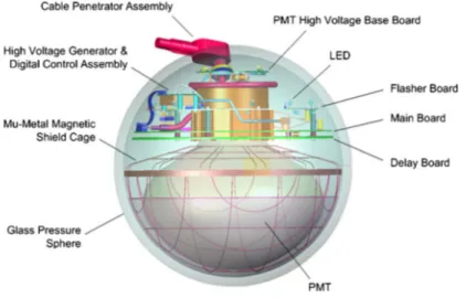
4.3 Detector Components . . . 60

4.3.1 The Digital Optical Module . . . 62

4.3.2 The Deep Antarctic Ice . . . 63

4.3.3 Data Acquisition and Online Filtering . . . 64

4.4 Detector Simulation . . . 65

4.5 Event Signatures . . . 67

4.6 Event Reconstruction . . . 67

4.6.1 Track Reconstruction . . . 69

4.6.2 Shower Reconstruction. . . 72

4.6.3 Relation to Neutrino Properties. . . 72

5 Atmospheric Backgrounds in Neutrino Telescopes 75 5.1 Atmospheric Muons . . . 77

5.1.1 Flux Characteristics . . . 77

5.1.2 Estimating the Background with Simulations . . 79

5.2 Atmospheric Neutrinos. . . 80

5.2.1 Flux Characteristics . . . 80

5.2.2 Modeling of the Background . . . 83

5.3 Rejection Techniques . . . 85

5.3.1 Selecting Upgoing Track Events. . . 85

5.3.2 Selecting Shower Events . . . 86

5.3.3 Vetoing Atmospheric Muons. . . 87

5.3.4 The Atmospheric Neutrino Self-Veto . . . 88

6 Searches for Cosmic Neutrinos with IceCube 91 6.1 Searches for a Diffuse Flux of Neutrinos . . . 93

6.1.1 Searches for Shower Events . . . 93

6.1.2 Searches for Track Events . . . 95

6.1.3 Hybrid Event Searches . . . 98

6.1.4 Effective Areas and Observable Distributions . . 98

6.2 Compilation of a Combined Event Sample . . . 100

7 A Likelihood Analysis on Multiple Event Samples 109 7.1 Modeling . . . 110

7.1.1 Background Components . . . 111

7.1.2 Cosmic Neutrino Component . . . 111

7.2 Likelihood Method . . . 114

7.2.1 Test Statistic . . . 114

7.2.2 Pseudo Experiments . . . 115

7.2.3 Likelihood Ratio Tests . . . 115

7.2.4 Construction of a Credible Energy Interval . . . 117

7.3 Systematic Uncertainties. . . 117

7.3.1 Energy Calibration Scale . . . 118

7.3.2 Spectral Index of the Primary Cosmic-Ray Flux 121 7.3.3 Normalization of the Muon Background . . . 122

7.3.4 Atmospheric Pion-to-Kaon Ratio . . . 122

7.4 Data Challenges . . . 122

7.4.1 Energy Spectrum . . . 123

7.4.2 Flavor Composition . . . 124

7.4.3 P-Values . . . 127

8 Results 131 8.1 Results on the Energy Spectrum . . . 132

8.1.1 Power Law Model . . . 132

8.1.2 Other Spectral Models . . . 142

8.1.3 North-South Model. . . 143

8.2 Results on the Flavor Composition . . . 145

8.2.1 2-Flavor Model . . . 145

8.2.2 3-Flavor Model . . . 145

9 Discussion and Outlook 149 9.1 Comparison to Previous Measurements. . . 150

9.1.1 Energy Spectrum . . . 150

9.1.2 Flavor Composition . . . 151

9.2 Implications of the Measurement Results. . . 153

9.3 Outlook . . . 154

10 Conclusion 159

A Time Consumption of Muon Background Simulation 164

B Extension of Event Sample S2 170

C Binning of Observables 172 D Comparison of Results with Restored Event Samples 174

Bibliography 177

List of Figures 209

List of Tables 213

Acknowledgements / Danksagung 215

Selbstst¨andigkeitserkl¨arung 217

Introduction

“I have done a terrible thing, I have postulated a particle that cannot be detected.”

— Wolfgang Pauli [1]

10¹⁴ 10¹⁵ 10¹⁶ 10¹⁷ 10¹⁸ 10¹⁹ 10²⁰ E [eV]

10¹³ 10¹⁴ 10¹⁵ 10¹⁶

E2.7×Φ[eV1.7 s−1sr−1cm−2]

“knee” “ankle”

Tibet Kascade Kascade Grande Tunka

IceTop

Telescope Array Auger

Figure 1.1 —The Energy Spectrum of Cosmic Rays. Shown are measure- ments of the all-particle cosmic-ray energy spectrum by the Tibet-III Air-Shower Array [2], the KASCADE experiment [3], the KASCADE- Grande experiment [4], the Tunka-133 EAS Cherenkov light array [5], IceTop [6], the Telescope Array [7] and the Pierre Auger Observatory [8].

Note that the vertical axis is scaled withE^2.7, to enhance the visibility of spectral features.

E

ventually, Wolfgang Pauliwas proven wrong. The neutrino, whose existence Pauli had postulated in a letter in 1930 [1], but of which he famously stated that it could not be detected, was in fact discovered in an experiment conducted by Frederick Reines and Clyde Cowan in 1953 [9]. It was not long after this that Kenneth Greisen and again Frederick Reines realized the neutrino’s potential as a cos- mic messenger: in 1960, both published articles in which they pointed out that neutrinos can be expected to be created in extraterrestrial environments, and that they propagate unaffected by cosmic magnetic fields or interstellar matter and hence carry unique information from their point of creation directly to the Earth [10,11]. Because of the technological challenge that neutrino detection presents, however, neu- trino astronomy remained wishful thinking for many decades.

In the meantime, great progress in understanding the high-energy Universe has been made through the observation of high-energy pho- tons and high-energy charged particles. Both reaching us from the depths of the cosmos, these are commonly referred to as gamma rays and cosmic rays, respectively. As an example, the energy spectrum of cosmic rays (predominantly ionized nuclei) as measured by present-day experiments is displayed infig. 1.1. While the exact transition point is still a matter of debate, it is generally acknowledged that cosmic rays with energies up to the “knee” are accelerated within the Milky Way, whereas cosmic rays with energies above the “ankle” are thought to be of extragalactic origin. This leads to the conclusion that both within and outside of our galaxy, cosmic rays are accelerated to remarkably high energies, certainly beyond the reach of any man-made accelera- tor. And yet, the acceleration sites of these particles have not been revealed until today.

It is well possible that the unambiguous identification of cosmic- ray acceleration sites is only achievable through the detection of high- energy neutrinos. These are inevitably produced when cosmic rays interact with ambient gas or photon fields, both of which are expected to be present at the acceleration sites. Unlike the cosmic rays, neu- trinos are not magnetically deflected on their way to the Earth, and unlike gamma rays, they are not produced in processes that do not involve high-energy nuclei, such as inverse Compton scattering. These properties make the neutrino an ideal cosmic messenger. The expected flux of cosmic neutrinos is small however, together with the low interac-

tion cross section of the neutrino this implies that very large detection volumes are needed to be able to record it.

Moisei Markov was the first to realize that natural detection media could be employed to accomplish this task. In 1960, he proposed “to install detectors deep in a lake or a sea and to determine the direction of charged particles with the help of Cherenkov radiation” [12] (as cited in [13]). The “charged particles” are created when neutrinos interact with nuclei in the water, and their directions are strongly correlated with those of the primary neutrinos. Several such “neutrino telescopes” have been conceived, some – like the DUMAND project off the coast of Hawaii [14] – were never put into effect, others – like the Baikal neutrino experiment in the lake Baikal in Siberia [15] or the ANTARES detector in the Mediterranean [16] – successfully take data to this day.

A new idea was published by Francis Halzen and John Learned in 1988: instead of deploying the detector under water, they proposed to utilize transparent, deep polar ice as a detection medium [17]. In 2000, a first detector of this concept, similar in size to the Baikal experiment and ANTARES, was finished near the Amundsen-Scott station at the geographical South Pole: AMANDA [18]. While all three detectors – the Baikal experiment, ANTARES and AMANDA – were successful in measuring atmospheric neutrinos, which constitute the most important background to searches for cosmic neutrinos, none of them was large enough to be able to detect a flux of cosmic neutrinos. However, they paved the way for larger successor experiments, one of which – the IceCube Neutrino Observatory – has already been put into operation.

The IceCube Neutrino Observatory is the successor experiment of AMANDA and has been installed at the same location over a period of 6 years from 2004 to 2010. With more than 5,000 optical sensors within a volume of roughly 1 km³ of deep Antarctic ice, it is by far the largest neutrino telescope that has ever been taken into operation, bringing the detection of cosmic neutrinos within reach for the first time. Indeed, only three years after the completion of the IceCube detector, and more than 50 years after the first proposals by Greisen, Reines and Markov, the IceCube Collaboration announced that it has found evidence for extraterrestrial neutrinos in 2013 [19]. The cosmic flux manifests itself as a deviation from the energy spectrum and zenith angle distribution expected of atmospheric neutrinos in the TeV–PeV

energy range (1 TeV = 10¹²eV; 1 PeV = 10¹⁵eV), and has in this way been confirmed in several follow-up searches [20–22]. In retrospect, it becomes evident that indications for this flux had already been vis- ible in earlier searches on data taken during the construction phase of IceCube [23–25]. The sources of the flux were searched for, but have escaped identification so far [20,26–30]. This suggests that there are numerous sources, none of which is currently strong enough to be detected above the background of atmospheric neutrinos by itself.

Nevertheless, it is possible to constrain the properties of these sources by analyzing the energy spectrum and the flavor composition of the neutrino flux they produce [31–35]. This is attempted in the present thesis.

To this effect, the energy spectrum and flavor composition of the cosmic neutrino flux in the TeV–PeV energy range are determined with a maximum-likelihood analysis in this work. Templates for back- ground and signal components, obtained through simulation, are fitted to the distributions of reconstructed energy, zenith angle, and particle signature recorded with the IceCube detector. Similar measurements have already been done [20–22,36], but were based on data sets much smaller than the one used here. The event samples used in this thesis were originally selected for individual studies [20–25] and were com- piled by the author for the purpose of this measurement. The work thus constitutes the first comprehensive analysis of IceCube data with regard to the energy spectrum and flavor composition of the cosmic neutrino flux.

The thesis is organized as follows: In chapter 2, the neutrino as a messenger particle is introduced. General properties and possible sources of a cosmic neutrino flux are discussed in chapter 3, while chapter 4gives an introduction to the IceCube Neutrino Observatory.

Chapter 5 outlines the atmospheric backgrounds that are specific to searches for cosmic neutrinos with IceCube. An overview of the differ- ent searches that have previously been performed is given inchapter 6, along with a characterization of the event samples that are used in this work. The likelihood framework that is used to simultaneously analyze these samples is introduced inchapter 7, the results of the analysis are presented inchapter 8. Chapter 9gives an interpretation of the results, as well as an outlook to results that can be expected to be obtained in the foreseeable future. Finally,chapter 10concludes the thesis.

The Neutrino as a Messenger Particle

“[...], which means that they propagate essentially unchanged in direction and energy from their point of origin [...] and so carry information which may be unique in character.”

— Frederick Reines (1960) [11]

10⁻⁶ 10⁻³ 10⁰ 10³ 10⁶ 10⁹ 10¹² 10¹⁵ 10¹⁸ 10²¹ E [eV]

10⁻³⁸ 10⁻³² 10⁻²⁶ 10⁻²⁰ 10⁻¹⁴ 10⁻⁸ 10⁻² 10⁴ 10¹⁰ 10¹⁶

Φ[eV−1 s−1sr−1cm−2]

CνB Solar Terrestrial

SN 1987a Diffuse SN

Atmospheric

GZK AGN

GRB

Figure 2.1 —Neutrinos from Natural Sources. Shown are predicted spec- tra of the cosmic neutrino background (CνB) [37], solar neutrinos [38], terrestrial neutrinos [39], the supernova 1987a and the diffuse super- nova neutrino background [40], atmospheric neutrinos [41], neutrinos from active galactic nuclei (AGN) [42–44] and from gamma ray bursts (GRB) [45], and cosmogenic neutrinos (GZK) [46].

T

he first important characteristic of the neutrino as a messen- ger particle is its extremely feeble interaction with other particles.

Because it does not carry electric charge, it is not subject to the elec- tromagnetic force. The neutrino can interact with matter via the weak force, but does so only with very low cross sections. This means that it can escape all but the densest environments, including, for example, the interior of the Sun. It also implies that neutrinos can reach the Earth from the farthest edges of the Universe, even if they carry a large energy. This distinguishes them from photons, which, with in- creasing energy, are more and more likely to get absorbed in electron pair-production interactions with ambient radiation fields, such as the cosmic microwave background. This “gamma-ray horizon”, from be- yond which photons are unlikely to reach the Earth, is depicted in fig. 2.2. Furthermore, the neutrino shares the photon’s property not to be affected by magnetic fields, thus traversing the cosmos without changing its direction. This is not the case for charged cosmic rays, which are deflected from their trajectories by the ever-present magnetic fields within and between galaxies.

The second feature that makes the neutrino an excellent messenger particle is its permanent emergence in a manifold of environments. Fig- ure 2.1 shows the energy spectra of a selection of naturally occurring neutrino species, ranging from the cosmological neutrino background at milli-electronvolts to the so-called cosmogenic neutrinos at more than 10¹⁸eV. Some of these neutrino species have successfully been observed, such as solar, terrestrial, and atmospheric neutrinos. In ad- dition, measurements with neutrinos that were artificially produced in reactors and accelerators have been performed. All of these mea- surements have yielded rich knowledge both about the sources of the neutrinos as well as the properties of the neutrinos themselves, showing the rich potential of the neutrino as a messenger particle. Section 2.1 introduces the fundamental properties of the neutrino that we know to- day, focusing on those that are relevant for this work. Section 2.2then gives a summary of the most important established neutrino sources and outlines the implications of essential measurements of neutrinos from these sources.

Other neutrino species have not been measured yet, but are theo- retically well established; these are briefly outlined insection 2.3. Of particular relevance for this thesis is the conjecture that, just like in

10⁻⁵ 10⁻³ 10⁻¹ 10¹ 10³ z

10⁷ 10⁸ 10⁹ 10¹⁰ 10¹¹ 10¹² 10¹³ 10¹⁴ 10¹⁵ 10¹⁶

E[eV] Galacticcenter Andromeda Mrk501

CMB infrared

visual UV

Figure 2.2 — The Gamma-Ray Horizon. The horizon is marked by the boundary of the gray area, as a function of the distance to the Earth, measured in cosmological redshiftz. Gamma-ray photons of a partic- ular energyE from beyond this horizon are likely to be absorbed by the radiation fields denoted by the labels in black font (CMB: cosmic microwave background; UV: ultra-violet radiation). Also indicated are the distances to the center of our Galaxy, the Andromeda galaxy, and the active galaxy Markarian 501. There is no corresponding horizon for neutrinos of the same energies. Reproduced from [47].

the Earth’s atmosphere, cosmic rays create neutrinos nearby their ac- celeration sites,i.e.that the sources of high-energy cosmic rays are also sources of high-energy neutrinos. Detecting a flux of neutrinos from these as yet unidentified sources, and thus to learn about their nature, is the primary target of neutrino telescopes like the IceCube Neutrino Observatory. Theoretical expectations and candidate sources for such a cosmic neutrino flux are presented in more detail inchapter 3.

2.1 Fundamental Properties of Neutrinos

The neutrino was hypothesized in 1930 by Wolfgang Pauli as a means to rescue the law of energy conservation, which appeared to be violated in measurements ofβ-decay spectra in the late 1920’s. The first theo- retical framework that contained the neutrino and its interactions was then formulated in Enrico Fermi’s famous paper “Versuch einer Theo- rie derβ-Strahlen” in 1934 [48], only four years after Pauli’s postulate, and long before it was first detected. Later, the neutrino became an integral component of the theory of the so-called Fermi (or weak) in- teraction, proposed by Sudarshan and Marshak [49] and Feynman and Gell-Mann [50] in 1958. Today, neutrinos and their interactions are described within the Standard Model of particle physics (for a general review, see [51]).

In the Standard Model, there are three generations of neutrinos:

the electron neutrino (νe), the muon neutrino (νµ), and the tau neu- trino (ντ), as well as their antiparticles (¯ν_e,¯ν_µ,ν¯_τ). The distinction between neutrinos and antineutrinos is unimportant for most of this work, the expressionneutrino stands for both unless explicitly noted.

Neutrinos are electrically neutral and subject only to weak interac- tions. Via the exchange of heavy gauge bosons (W^± and Z⁰), they can interact with the other fermions of the Standard Model, i.e.the charged leptons (the electron, muon, and tau) and the quarks. The basic Feynman diagrams for these interactions are shown in fig. 2.3.

According to the electric charge of the mediator, the interactions are called charged-current (W^±) and neutral-current (Z⁰) interactions. In charged-current interactions, due to charge conservation, neutrinos are transformed into the corresponding charged leptons: electron neutri- nos into electrons, muon neutrinos into muons, and tau neutrinos into tau leptons. In contrast, no particle transformation takes place in neutral-current interactions.

While neutrinos are massless in the original formulation of the Stan- dard Model, the observation of neutrino oscillations (for a summary see section 2.1.3) suggests that neutrinos do have mass. Experiments aiming at measuring the neutrino mass have been carried out, but have only provided upper limits so far. The currently most strin- gent, although model-dependent upper limits are obtained indirectly by cosmological and astrophysical measurements; these constrain the

l W

q,l q,

(a)

Z

q,l q,l

(b)

Figure 2.3 —Feynman Diagrams for Neutrino Interactions. (a)charged- current interaction;(b)neutral-current interaction. q denotes quarks, l charged leptons. Note that in charged-current interactions, initial and final state particles are not identical.

sum of all neutrino masses to be smaller than 0.2−1.3 eV, depending on the measurement technique [52]. More directly, measurements of the endpoint of the β-decay spectrum have provided upper limits of

∼2 eV on the average electron neutrino mass [53]. Employing the same technique, the KATRIN experiment, currently under construction, is designed to be sensitive down to 0.2 eV [53].

Given these restrictive upper limits, neutrinos can be treated as massless for all practical purposes other than neutrino oscillations in excellent approximation. In this case, the neutrino’shelicity

h=~s·~p

|~p| , (2.1)

i.e. the projection of its spin~sonto its momentum ~p, is a conserved quantity. Furthermore, the helicity coincides with the chirality, or handedness, of the neutrino, which governs its interaction with other particles. Experimentally, only neutrinos with helicity h = −1 and antineutrinos with helicityh= 1 have been observed so far; this was first found by Goldhaberet al. [54] and Palathingal [55], respectively.

Therefore, in the Standard Model, neutrinos interact always as left- handed particles and antineutrinos always as right-handed particles.

2.1.1 Neutrino Production Processes

Neutrinos are produced in a variety of processes, very often in the decay of other particles. For instance, the muon and tau are both unstable and their decay products always include neutrinos. The muon virtually always decays into an electron, an electron antineutrino and a muon neutrino (or their antiparticles):

µ⁻ → e⁻+ ¯νe+ν_µ;

µ⁺ → e⁺+νe+ ¯ν_µ. (2.2) The tau has many decay modes, all containing at least one tau neutrino in the final state. Furthermore, electron and muon neutrinos are pro- duced in the main decay modes, either directly or indirectly through the decay of secondary pions (seeeq. 2.4) [51].

Neutrinos are also often produced in the weak decay of hadronic particles,i.e.particles consisting of quarks. The classic example is the beta decay of the neutron,

n → p + e⁻+ ¯ν_e, (2.3)

in which electron antineutrinos are produced. Heavier atomic nuclei can also undergo beta decay, always leading to the production of elec- tron antineutrinos. Decay modes of heavier baryons that include neu- trinos often have very small branching fractions [51].

Another example of neutrino production by the decay of hadronic particles is meson decay. The lightest meson is the pion; charged pions almost exclusively decay into a muon and a muon neutrino:

π⁻ → µ⁻+ ¯ν_µ;

π⁺ → µ⁺+ν_µ. (2.4)

Heavier mesons often have multiple decay modes, many of which con- tain neutrinos in the final state [51].

Finally, it should be mentioned that neutrinos are also created in nuclear fusion processes,e.g.in the Sun. In contrast to neutrinos pro- duced in particle decays, which are limited in energy only by the energy of the mother particle, neutrinos created in fusion processes carry en- ergies not larger than ∼ 20 MeV [38], and are thus not important in the scope of this thesis.

2.1.2 Neutrino Interactions at High Energies

Of particular interest for this work is the interaction of high-energy neutrinos with nucleons. For a general overview on neutrino interac- tions, seee.g.[56].

In neutrino-nucleon interactions, neutrinos with energies&10 GeV can resolve the constituents of the nucleon and scatter off individual quarks. This process is called deep inelastic scattering (DIS) and is by far the dominant interaction process for neutrinos in the energy range relevant to this work, Eν &1 TeV [56] (with the partial exception of the Glashow resonance, see further below). Figure 2.4shows Feynman diagrams of charged-current and neutral-current DIS processes. In both cases, the interacting nucleus is ripped apart, giving rise to a hadronic particle shower. In addition, the final state contains either a charged lepton or, in neutral-current interactions, a neutrino.

l

X N

W

(a)

X N

Z

(b)

Figure 2.4 —Feynman Diagrams for Deep Inelastic Scattering.

(a)charged-current interaction; (b) neutral-current interaction. N de- notes the interacting nucleon, X symbolizes a hadronic particle shower.

The cross sections for scattering of neutrinos with nucleons at high energies are shown in fig. 2.5. Up to energies of∼10¹³eV, the cross section grows linearly with the neutrino energy and is larger for neutri- nos than for antineutrinos; the latter is a consequence of the opposite helicities of neutrinos and antineutrinos [56]. At higher energies, the energy transferred in the interaction by the intermediate boson can no

longer be neglected with respect to its mass, this leads to a suppression of the cross section and disperses the difference between neutrinos and antineutrinos [56].

Figure 2.5also shows the cross section for the scattering of electron antineutrinos with electrons. As first pointed out by Glashow, this process has a resonance when the center-of-mass energy of the system reaches the mass of the mediating boson [57]. For electrons at rest and the mass of the W^± boson mW = 80.4 GeV, the Glashow reso- nance occurs at a neutrino energy of 6.3×10¹⁵eV. As can be seen from the figure, the interaction probability for electron antineutrinos is dramatically enhanced at this energy.

10¹² 10¹³ 10¹⁴ 10¹⁵ 10¹⁶ 10¹⁷ 10¹⁸ E [eV]

10⁰ 10¹ 10² 10³ 10⁴ 10⁵ 10⁶

σ[pb]

CC NC

¯ νe+ e⁻

ν+ N

¯ ν+ N

Figure 2.5 —Neutrino Cross Sections at High Energies. Cross sectionσ for charged-current (blue) and neutral-current (orange) neutrino-nucleon scattering of neutrinos with energyE. The cross section for the scat- tering of electron antineutrinos with electrons is shown in purple, this process is dominant around the so-calledGlashow resonanceat 6.3 PeV.

Reproduced from [58].

2.1.3 Neutrino Oscillations

Neutrino oscillations refers to the phenomenon that neutrinos can change their type – or flavor – during propagation: there is a non- zero probability that a neutrino produced with a particular flavor is detected as another flavor. It was first pointed out by Pontecorvo that this possibility occurs if neutrinos have mass [59]. As neutrino oscilla- tions have been observed, it is generally acknowledged today that this must be the case. The Standard Model, assuming massless neutrinos, is hence incomplete in this respect. It can however be extended to in- clude massive neutrinos, where two general cases can be distinguished:

(i) the neutrino could be a so-called Dirac fermion, acquiring mass in the same way as the other fermions, i.e. the charged leptons and quarks; (ii) the neutrino could be a Majorana fermion, acquiring mass by a different mechanism that is based on the conception that neu- trinos and antineutrinos are identical. The latter is a possibility that exists because neutrinos are, in contrast to all other fermions, electri- cally neutral. For more details on the acquirement of neutrino masses, seee.g.[60]. In the following derivations, it is assumed that neutrinos are Dirac fermions; this choice has no impact on any conclusions drawn here.

The theory of neutrino oscillations in vacuum is briefly outlined in this section, following the review in [61]. Neutrino oscillations in mat- ter are not relevant for the present work and are not covered here. In the following, natural units are used (~=c= 1).

The basic conditions for neutrino oscillations to occur is that

• there are three neutrinomass eigenstates|ν1i,|ν2i,|ν3iwith dif- ferent masses;

• the mass eigenstates do not coincide with the flavor eigenstates

|νei,|ν_µi,|ν_τi.

While the flavor eigenstates are defined by the neutrino production and interaction processes, the propagation of neutrinos is governed by the mass eigenstates. The flavor eigenstates and mass eigenstates are connected by the transformation

|ναi=X

j

U_αj^∗ |νji, (2.5)

withα= e,µ,τandj= 1,2,3. The unitary rotation matrixU is called Pontecorvo-Maki-Nakagawa-Sakata (PMNS) matrix, named after pio- neers of the theory. It is commonly parametrized as

U =





c12c13 s12c13 s13e^−iδ

−s12c23−c12s13s23e^iδ c12c23−s12s13s23e^iδ c13s23

s12s23−c12s13c23e^iδ −c12s23−s12s13c23e^iδ c13c23



, (2.6) where sjk ≡sinθjk andcjk ≡cosθjk. The matrix hence depends on four independent parameters, three mixing angles (θ12, θ13, and θ23) and one phase parameter (δ).

The temporal evolution of the mass eigenstates is given by the Schr¨odinger equation, which, for particles propagating in vacuum, has the solution

|νj(t)i=e^−iEjt|νj(t= 0)i, (2.7) wheretdenotes the time andEj the energy of the neutrino (using the so-calledplane wave approximation, seee.g.[61] and references therein for more details).

The probability to detect a neutrino with initial state|ναias state

|νβiis then

Pνα→νβ =

νβ|e^−iEjt|να

2=

X

j

U_αj^∗ Uβj e^−iEjt

2

=X

j,k

U_αj^∗ UβjUαkU_βk^∗ e^{−i(Ej−Ek)t}. (2.8) Using the fact that neutrinos are ultra-relativistic for all cases consid- ered here, we can now simplify

Ej = q

p²_j+m²_j ' pj+m²_j

2pj ' E+m²_j

2E (2.9)

andt'L, whereLis the propagation distance of the neutrino. This leads to

−i(Ej−Ek)t ' −i∆m²_jkL

2E , (2.10)

with the squared mass differences ∆m²_jk≡m²_j−m²_k. Using this,eq. 2.8 can be written as

Pνα→νβ =δαβ−4X

j>k

Re U_αj^∗ UβjUαkU_βk^∗

sin² ∆m²_jkL 4E

!

+ 2X

j>k

Im U_αj^∗ UβjUαkU_βk^∗

sin ∆m²_jkL 2E

! ,

(2.11)

where δαβ is the Kronecker delta function. The oscillatory phase can conveniently be expressed as

∆m²_jkL

4E ≈ 1.267×∆m²_jk eV²

L km

GeV

E . (2.12)

Fromeq. 2.11it may now be observed that the oscillation probability depends on the four parameters of the PMNS matrix U, the squared mass differences ∆m²_jk, and the ratio of the propagation distance to the neutrino energy, L/E. While the latter is determined by the ex- perimental setup, the other parameters are fundamental and have to be determined experimentally. This has been achieved to reasonable precision for all parameters except the phase parameterδ, seetable 2.1 for an overview.

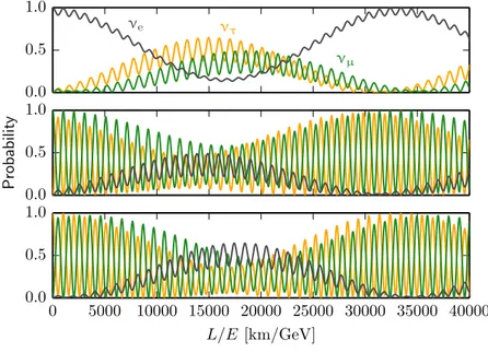
A graphical illustration of the effect of neutrino oscillations may be obtained fromfig. 2.6, which shows the oscillation probability (eq. 2.11) for the different neutrino flavors as a function of theL/Eparameter.

If multiple neutrinos from a source are observed, coherence effects become important. Specifically, if the neutrinos are produced incoher- ently (i.e.out of phase) and travel sufficiently far, the probability to observe a particular neutrino flavor (eq. 2.11) must be averaged over L/E:

hPνα→νβi=δαβ−2X

j>k

Re U_αj^∗ UβjUαkU_βk^∗

. (2.13) This probability is now independent of the squared mass differences

∆m²_jk as well as independent of the propagation distance L and the neutrino energyE. Hence, in an incoherently produced neutrino beam, the probability to observe a particular flavor is fully determined by the input energy spectrum and flavor composition of the neutrinos.

Table 2.1 — Neutrino Oscillation Parameters. Best-fit neutrino oscilla- tion parameters as determined in [62]. Note that the sign of ∆m²₃₂is yet unknown, the table gives the best-fit values assuming so-called normal ordering (∆m²₃₂>0;m1< m2< m3) and inverted ordering (∆m²₃₂<0;

m3 < m1 < m2) separately. The inverted ordering is slightly preferred in [62], although with very low significance.

Parameter / Unit Normal ordering Inverted ordering θ12/^◦ 33.48^+0.78_−0.75 33.48^+0.78_−0.75 θ13/^◦ 8.50^+0.20_−0.21 8.51^+0.20_−0.21 θ23/^◦ 42.3^+3.0_−1.6 49.5^+1.5_−2.2

δ /^◦ 306⁺³⁹₋₇₀ 254⁺⁶³₋₆₂

∆m²₂₁/10⁻⁵eV² 7.50^+0.19_−0.17 7.50^+0.19_−0.17

∆m²₃₂/10⁻³eV² 2.457^+0.047_−0.047 −2.449^+0.048_−0.047

2.2 Established Neutrino Sources

This section gives a short overview of measurements of neutrinos from known sources, showing how neutrinos were employed as messenger particles in the past (and still are today). The existence of three gen- erations of neutrinos and many of their fundamental properties have been determined in experiments with artificially produced neutrinos, seesection 2.2.1. The only identified source of neutrinos from beyond the solar system is SN 1987a, a supernova explosion that took place in the Large Magellanic Cloud in 1987 (section 2.2.2). Finally, the fact that neutrinos can oscillate,i.e.change their flavor during propagation, was established in measurements of solar and atmospheric neutrinos, as summarized insection 2.2.3andsection 2.2.4.

2.2.1 Artificially Produced Neutrinos

The two most important classes of artificially produced neutrinos are reactor neutrinos and accelerator neutrinos, which are explained in this section. Significant numbers of neutrinos are also produced in the explosion of nuclear weapons, this is not discussed here.

0.0 0.5 1.0

νe

νµ

ν_τ

0.0 0.5 1.0

Probability

0 5000 10000 15000 20000 25000 30000 35000 40000 L/E[km/GeV]

0.0 0.5 1.0

Figure 2.6 — Neutrino Oscillation Probabilities. Shown are the prob- abilities for an initial electron neutrino (top), muon neutrino (center), and tau neutrino (bottom) to be detected as an electron neutrino (gray), muon neutrino (green), or tau neutrino (yellow) as a function of the pa- rameterL/E. Calculated witheq. 2.11, using the neutrino oscillations parameters intable 2.1(inverted ordering).

Reactor Neutrinos

In nuclear reactors, energy is released by nuclear fission of heavy iso- topes. The fission fragments undergo beta decay (see eq. 2.3), thus producing some 10²⁰ electron antineutrinos per second in a typical re- actor [63]. A fraction of these neutrinos can then be detected via the inverse beta decay reaction

¯

νe+ p → e⁺+ n. (2.14)

In their pioneering experiment in 1953, Reines and Cowan used a de- tector filled with cadmium-loaded scintillator to identify reactions of this kind, where the coincident detection of a prompt scintillation sig-

nal from the positron and a delayed signal from neutron capture on cadmium provided a unique signature [9]. This experiment constituted the first detection of the neutrino, thus confirming Pauli’s postulate.

Today, experiments with very similar techniques are still performed at different nuclear reactors around the world. Recently, these exper- iments have provided the first measurement of the neutrino mixing angleθ13[64,65], one of the few remaining unknown parameters in the theory of neutrino oscillations.

Accelerator Neutrinos

Neutrinos can also be produced by colliding high-energy protons with a massive target. The secondary products of such collisions include charged pions, which decay into a muon and a muon neutrino (see eq. 2.4). In 1962, the muon neutrino was first detected in an experiment located at an accelerator at the Brookhaven National Laboratory [66].

The muons produced in the pion decay were stopped in a thick iron wall before they could decay; the neutrinos were detected in a spark chamber behind the wall. Unlike in the case of the electron neutrino, in which electrons are produced in the interaction, muons were found as interaction products. This lead to the important conclusion that there are more than one type of neutrinos.

Similarly, the tau neutrino was discovered in an accelerator exper- iment in 2000, this time originating from the decay of DS mesons that were created in the collision of a proton beam with a tungsten target [67]. With this discovery three generations of neutrinos were established, matching the three generations of charged leptons and quarks that had been detected by this time.

Nowadays, accelerator neutrinos are being employed to perform pre- cision measurements of neutrino oscillations. In particular, the first experiments that have measured neutrinos of a flavor different from the one produced (so-calledappearance experiments) were recently carried out with accelerator neutrinos [68,69].

2.2.2 Neutrinos from the Supernova Explosion SN 1987a On February 23, 1987, a burst of neutrino events was observed in three different underground neutrino detectors, located in Japan, the

United States, and the Soviet Union, within a time interval of less than a minute [70–72].¹ The sequence of the neutrino arrival times and energies is shown infig. 2.7. Even though only 24 neutrinos were detected in total, the expected background within the detection time window was much lower, so that the detection was highly significant.

0 20 40

E[MeV] Kamiokande

0 20 40

E[MeV] IMB

7 : 35 : 35 7 : 35 : 45 7 : 35 : 55 7 : 36 : 05 7 : 36 : 15 7 : 36 : 25 Time on Feb 23, 1987 (UT)

0 20 40

E[MeV] Baksan

Figure 2.7 — Neutrinos from SN 1987a. Time sequence showing the arrival times and energies of the neutrino events detected in the Kamiokande detector in Japan [70], the IMB detector in the United States [71], and the Baksan detector in the Soviet Union [72]. Note that the times of the events in the Kamiokande detector are uncertain to

±1 minute and the times of the events in the Baksan detector have an uncertainty of⁺²₋₅₄ seconds [75].

One day later, on February 24, a core-collapse supernova explosion (named SN 1987a) was discovered in the Large Magellanic Cloud, a satellite galaxy of the Milky Way. Since core-collapse supernovae are

1Another detector located at the French-Italian border also reported the detection of several neutrinos [73]. However, since these neutrinos were detected several hours prior to those in the other three experiments, their origin is questionable (see [74]).

expected to release about 99% of the available energy by emitting a short burst of∼10⁵⁸neutrinos [76], it is very likely that the neutrinos detected on the previous day originated from the supernova explosion.

This is remarkable because SN 1987a remains the only identified object outside the solar system from which neutrinos have been detected as of this writing. The observations of the neutrino burst are in accordance with basic models for core-collapse supernova explosions [74], showing that our theoretical understanding of these phenomena is solid.

2.2.3 Solar Neutrinos

In the Sun, neutrinos are a product of the nuclear fusion process. The majority of the neutrinos are produced in the pp-reaction

p + p → d + e⁺+ν_e, (2.15) with energies of up to 0.4 MeV. These neutrinos are produced so abun- dantly that∼60 billion pass through every square centimeter per sec- ond at Earth [38]. Fewer, yet still numerous neutrinos with energies of up to 15 MeV are created in the decay of boron-8 in the Sun,

8B → ⁸Be + e⁺+νe. (2.16) Note that only electron neutrinos are produced in the Sun.

The first attempt to measure neutrinos from the Sun was made by Ray Davis at the end of the 1960’s in an experiment located in the Homestake gold mine in South Dakota [77]. He employed a large tank filled with perchloroethylene, or C2Cl4, a common cleaning fluid. Upon interaction with electron neutrinos, chlorine atoms in the fluid con- verted into radioactive argon isotopes,

νe+ ³⁷Cl → ³⁷Ar + e⁻, (2.17) which were collected and counted. Because the expected count rates were very low, the experiment was conducted over a very long time un- til 1995. Famously, the rate of solar neutrinos measured by Davis was only about one third of that predicted by the standard solar model [78].

This discrepancy between the theoretical prediction and the measure- ment of solar neutrinos became known as the solar neutrino problem.

A different technique was employed by the Kamiokande experiment and its successor experiment Super-Kamiokande, which is still running today. The Super-Kamiokande detector consists of a large tank of ultra-pure water, viewed by more than 10,000 photomultiplier tubes [79]. Neutrinos of any type α can be detected via neutrino-electron scattering,

να+ e⁻ → να+ e⁻ (2.18)

where the sensitivity to electron neutrinos is larger because both neu- tral and charged-current interactions are possible. Because also the direction of the incident neutrinos can be determined, it was possi- ble for the first time to demonstrate that the detected neutrinos were coming from the direction of the Sun. Nevertheless, the rate of solar neutrinos that was measured was only 36% of the predicted rate [80], enhancing the solar neutrino problem further.

The problem was finally solved in 2001 by the Sudbury Neutrino Observatory (SNO), an experiment installed in a mine in Sudbury, Canada. While similar in design to the Super-Kamiokande detector, instead of normal water, the target material of the SNO detector con- sisted of heavy water, D2O. In addition to the electron scattering re- action (eq. 2.18), neutrinos could be detected by charged-current and neutral-current interactions with deuterons,

νe+ d → e⁻+ p + p ;

ν_α+ d → ν_α+ n + p, (2.19) where α can again be any neutrino flavor. Thus, the SNO detector was able to measure the charged-current interaction rate of electron neutrinos and, independently, the combined neutral-current interaction rate of all three neutrino flavors [81]. While the SNO experiment, like the other experiments, measured a deficit of electron neutrinos compared to the predictions, the inferred flux of all neutrino flavors was compatible with the predicted electron neutrino flux [82]. This was convincing evidence that solar neutrinos oscillate, changing their flavor on the way to Earth from electron neutrinos to muon and tau neutrinos.

Thus, after many years of debate, the observation of solar neutrinos not only has shown that the common understanding of the fusion pro-

cess in the Sun is correct, but also has revealed fundamental properties of the neutrino itself.

2.2.4 Atmospheric Neutrinos

The atmosphere of the Earth is constantly bombarded by cosmic rays, charged particles that can reach very high energies (cf.fig. 1.1). When such a cosmic ray hits an atom in the atmosphere, a cascade of sec- ondary particles is created, called an air shower. These secondary particles include charged pions, which eventually produce electron and muon neutrinos in their decay (see eq. 2.2 and 2.4). These neutri- nos, as well as those produced in the decay of other particles created in air showers, are referred to as atmospheric neutrinos. Because the primary cosmic rays may carry very large energies, atmospheric neu- trinos can reach much higher energies than those produced artificially, in supernovas, or in the Sun [83] (cf.fig. 2.1).

Atmospheric neutrinos were first detected in 1965 in two experiments that were independently carried out by two different groups. Both groups used scintillation detectors deep underground, one in a gold mine in India [84], the other in a gold mine in South Africa [85]. The large material overburden suppressed the background of cosmic-ray induced muons to a very small level, so that in both experiments only a handful of neutrino events were sufficient to claim the detection of atmospheric neutrinos.

Since the spectrum of cosmic rays is well measured, the spectrum of atmospheric neutrinos can be inferred, too (see e.g.[83]). In 1998, the Super-Kamiokande experiment, already introduced in the previous section, measured a significant deviation from these predictions [86].

Specifically, a deficit of atmospheric muon neutrino events from cer- tain directions was observed, while the measurement agreed with pre- dictions in other directions. The deficit was consistent with the inter- pretation that the neutrinos change their flavor as a function of the propagation distance, the measurement therefore constituted the first solid evidence for neutrino oscillations (although measurements of so- lar neutrinos had indicated this since long before, as summarized in the previous section).

For neutrino telescopes such as the IceCube Neutrino Observatory, atmospheric neutrinos are of importance as they constitute a back-

ground to searches for cosmic neutrinos, but also because they can be used as a calibration signal. In fact, as displayed in fig. 2.8, mea- surements of the atmospheric neutrino flux were performed with the IceCube experiment, but alsoe.g.with the Fr´ejus experiment and the ANTARES neutrino telescope. Atmospheric neutrinos as a background in neutrino telescopes are discussed further in chapter 5.

10⁰ 10¹ 10² 10³ 10⁴ 10⁵ 10⁶

E[GeV]

10⁻⁹ 10⁻⁸ 10⁻⁷ 10⁻⁶ 10⁻⁵ 10⁻⁴ 10⁻³ 10⁻² 10⁻¹

E2×Φ[GeVs−1sr−1cm−2]

Fr´ejusνµ

ANTARESνµ

IceCube-59ν_µ

Fr´ejus νe

IceCube-79 νe

Figure 2.8 — Measurements of the Atmospheric Neutrino Flux. Shown are measurements of the atmospheric neutrinos flux from the Fr´ejus ex- periment [87], ANTARES [88], and IceCube [89,90]. The vertical axis is scaled withE² for better readability.

2.3 Predicted Neutrino Sources

Several species of neutrino sources have been predicted but not yet (directly) detected. Some of these species are theoretically firmly es- tablished, others are more speculative. One species of particular inter- est for this work – neutrinos from the sources of high-energy cosmic

rays – is discussed in the following chapter. This section gives a short overview over other undetected sources, where the interested reader is referred to the provided references.

2.3.1 The Cosmic Neutrino Background

Analogous to the cosmic microwave background (CMB), the Universe is also filled with relic neutrinos from the Big Bang, the cosmic neu- trino background (CνB) [37]. These neutrinos have not been measured directly, however, their properties are well constrained by cosmologi- cal measurements, e.g.of the CMB [91]. The number density of the CνB is expected to be∼112 cm⁻³ and the average neutrino momen- tum is ∼ 5×10⁻⁴eV [92] (cf. fig. 2.1). While several methods to directly detect the CνB have been proposed (e.g. via the mechanical force induced by elastic scattering of relic neutrinos, via the capture of relic neutrinos on radioactive nuclei, or via absorption features in ultra-high-energy neutrino spectra), current experimental techniques still fall short several orders of magnitude of the required sensitivity (see [92] and references therein).

2.3.2 The Diffuse Supernova Neutrino Background

As already noted in section 2.2.2, supernova explosions of type II release a large fraction of their gravitational energy into a burst of

∼10⁵⁸ neutrinos with energies of some tens of MeV [76]. Such events are observable in neutrino detectors on Earth if the explosion takes place within or close to the Milky Way galaxy, as in the case of SN 1987a. Supernova explosions of type II in other galaxies produce a cu- mulative flux of neutrinos that arrive isotropically at Earth, referred to as diffuse supernova neutrino background (DSNB). Based on models for core-collapse supernova, expectations for the magnitude of this flux have been derived [40]. The DSNB has not been measured experimen- tally yet, but it has been argued that its detection may be in reach for current-generation neutrino experiments [93].

2.3.3 Neutrinos from Dark Matter Annihilation or Decay There is compelling indirect evidence that a large fraction of the matter in the Universe is “dark”,i.e.consists of particles beyond the Standard

Model of particle physics that do not participate in the electromagnetic interaction (for a review, see [94]). If these dark matter particles exist and have sufficient mass, they could annihilate or decay into known standard-model particles that would produce neutrinos in their sub- sequent decay chains, where the energy of the neutrinos is bounded by the dark matter particle mass. Many models predict masses in the GeV–TeV range, but models including much heavier particles have also been proposed [94].

Dark matter particles could accumulate in regions of large den- sity, such as the Sun or the center of galaxies, leading to enhanced annihilation rates and hence to an enhanced flux of neutrinos from there [95–97]. While many other regions of high dark matter density can also be probede.g.with photons, dark matter annihilation in the Sun can only be probed with neutrinos. The current best limit on the annihilation rate of dark matter particles in the Sun was obtained with the IceCube Neutrino Observatory [98].

High-energy neutrinos could also be produced in the decay of dark matter particles, if these are unstable. Such scenarios have been dis- cussed for dark matter particles with masses up to 10 TeV [99] as well as for extremely heavy dark matter particles [100,101].

Neutrinos from the Acceleration Sites of Cosmic Rays

“Space is big.

You just won’t believe how vastly, hugely, mind-bogglingly big it is.”

— Douglas Adams (1979) [102]

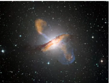
Figure 3.1 — Composite Image of the Active Galaxy Centaurus A. Sub- millimetre data (λ= 870µm) are shown in orange, X-ray data in blue.

Credit: ESO / WFI (Optical); MPIfR / ESO / APEX / A.Weisset al.

(Submillimetre); NASA / CXC / CfA / R.Kraftet al.(X-ray).

T

he paradigm ofhigh-energy¹neutrino astronomy rests upon one observational fact and two subsequent assumptions. The obser- vational fact is that cosmic rays (i.e.ionized nuclei) of immensely high energies reach the Earth from the cosmos (cf. fig. 1.1). The two as- sumptions are

(i) that these cosmic rays obtain their high energies through accel- eration in astrophysical environments; and

(ii) that they undergo interactions with other particles within or close to these environments.

If both assumptions hold, high-energy neutrinos are produced in conjunction with the cosmic rays and, being neutral particles, will propagate to the Earth in straight lines. In this case, their detection would offer a promising opportunity to uncover the acceleration sites of high-energy cosmic rays and to probe astrophysical acceleration pro- cesses.

Observations supportive of the first assumption include that the ac- celeration of charged particles has been observed at the Sun (up to energies of a few GeV, for a review seee.g.[103]), and that the signa- ture of pion decay has been observed with gamma rays in two super- nova remnants, which implies cosmic-ray acceleration up to TeV ener- gies [104]. Furthermore, as already noted in 1934 by Walter Baade and Fritz Zwicky [105,106], the observed intensity of cosmic rays can be sustained by supernova explosions in the Milky Way if these convert a few percent of their explosion energy into high-energy cosmic rays (see e.g.[107]).²

The second assumption is easily motivated when bearing in mind that the Universe is filled with gas clouds and radiation fields such as starlight or the cosmic microwave background radiation; in fact, it is hard to imagine an acceleration environment without ambient matter or photons. For these reasons, it is commonly expected that high- energy neutrinos reach us from the sources of high-energy cosmic rays (seee.g.[108]).

1In the context of this work, “high-energy” means energies larger than 1 TeV (10¹²eV).

2Note that this argument does not apply to the highest-energy cosmic rays, which are believed to be of extragalactic origin.

Experiments like the IceCube Neutrino Observatory have been de- signed to detect this flux of high-energy neutrinos, and eventually to re- solve its sources, the cosmic-ray acceleration sites. Before introducing the detector in the next chapter, it is instructive to review the expected general properties of a neutrino flux from cosmic sources (insection 3.1) and introduce some specific source candidates (insection 3.2).

3.1 General Considerations

3.1.1 Production Mechanisms

The vast majority of high-energy cosmic rays are either protons or heavier ionized nuclei. These particles can produce neutrinos when they interact with ambient target particles or radiation. The properties of the produced neutrino flux depend on the primary cosmic-ray flux as well as the properties of the target. There are two classes of targets generally considered, these are discussed in the following.

If the acceleration site is surrounded by interstellar gas clouds, the accelerated cosmic rays will collide with gas nuclei, producing neutral and charged pions in inelastic scattering processes. In the simplest case, both interacting nuclei are protons; hence this neutrino produc- tion mechanism is referred to as pp scenario (or, more general,hadronu- clearscenario). While the neutral pions give rise to high-energy gamma rays,

π⁰ → γ+γ, (3.1)

the charged pions produce neutrinos in their decay (cf.eq. 2.2and2.4), π⁺ → µ⁺+ν_µ → e⁺+ν_e+ ¯ν_µ+ν_µ;

π⁻ → µ⁻+ ¯ν_µ → e⁻+ ¯ν_e+ν_µ+ ¯ν_µ. (3.2) The simultaneous production of gamma rays and neutrinos implies a very tight connection between these two messenger particles in the pp scenario.

The other possibility is the so-called pγor photohadronic scenario.

In this case, the target for the high-energy cosmic rays are photons from radiation fields that are present at the acceleration sites (e.g.ambient