Virtual fatigue diagnostics of wake-affected wind turbine via Gaussian Process Regression

Research Collection

Journal Article

Virtual fatigue diagnostics of wake-affected wind turbine via Gaussian Process Regression

Author(s):

Avendaño Valencia, Luis David; Abdallah, Imad; Chatzi, Eleni Publication Date:

2021-06

Permanent Link:

https://doi.org/10.3929/ethz-b-000470688

Originally published in:

Renewable Energy 170, http://doi.org/10.1016/j.renene.2021.02.003

Rights / License:

Creative Commons Attribution-NonCommercial-NoDerivatives 4.0 International

This page was generated automatically upon download from the ETH Zurich Research Collection. For more information please consult the Terms of use.

ETH Library

Virtual fatigue diagnostics of wake-affected wind turbine via Gaussian Process Regression

Luis David Avenda~ no-Valencia ^{a , 1} , Imad Abdallah ^{b , * , 1} , Eleni Chatzi ^b

a

Department of Mechanical and Electrical Engineering University of Southern Denmark, Campusvej 55, 5230, Odense M, Denmark

b

Institute of Structural Engineering, ETH Zurich, Switzerland

a r t i c l e i n f o

Article history:

Received 8 November 2020 Received in revised form 31 January 2021 Accepted 1 February 2021 Available online 8 February 2021

Keywords:

Wind turbine Fatigue Wake Uncertainty

Bayesian Gaussian process regression Virtual sensing

a b s t r a c t

We propose a data-driven model to predict the short-term fatigue Damage Equivalent Loads (DEL) on a wake-affected wind turbine based on wind field inflow sensors and/or loads sensors deployed on an adjacent up-wind wind turbine. Gaussian Process Regression (GPR) with Bayesian hyperparameters calibration is proposed to obtain a surrogate from input random variables to output DELs in the blades and towers of the up-wind and wake-affected wind turbines. A sensitivity analysis based on the hyperparameters of the GPR and Kullback-Leibler divergence is conducted to assess the effect of different input on the obtained DELs. We provide qualitative recommendations for a minimal set of necessary and suf fi cient input random variables to minimize the error in the DEL predictions on the wake-affected wind turbine. Extensive simulations are performed comprising different random variables, including wind speed, turbulence intensity, shear exponent and inflow horizontal skewness. Furthermore, we include random variables related to the blades lift and drag coef fi cients with direct impact on the rotor aero- dynamic induction, which governs the evolution and transport of the meandering wake. In addition, different spacing between the wind turbines and W€ ohler exponents for calculation of DELs are considered. The maximum prediction normalized mean squared error, obtained in the tower base DELs in the fore-aft direction of the wake affected wind turbine, is less than 4%. In the case of the blade root DELs, the overall prediction error is less than 1%. The proposed scheme promotes utilization of sparse structural monitoring (loads) measurements for improving diagnostics on wake-affected turbines.

© 2021 The Author(s). Published by Elsevier Ltd. This is an open access article under the CC BY-NC-ND license (http://creativecommons.org/licenses/by-nc-nd/4.0/).

1. Introduction

The load effects and degradation of structural components of wind turbines (WTs) do not uniformly evolve across a wind farm due to, largely, wake effects and variability in the in fl ow conditions (and waves for offshore wind farms [27]). The assessment of fatigue damage accumulation on assumption of availability of direct load effects measurements on all main structural components across all wind turbines within a wind farm is not realistic. The assumption of availability of high- fi delity aero-servo-elastic simulators of the investigated wind turbines coupled to site-speci fi c in fl ow and wake models is convenient, but often not borne out of the actual reality experienced by wind farm owners and operators. At best, the designer/manufacturer of the wind turbine might make a single

comprehensive one-off set of output load effects of such wind farm simulations available to the owner/operator of the wind farm.

A further and, from the view of this paper, perhaps more important hindrance lies in the precise estimation of structural response signals that are typically not available in the standard data emanating from the Supervisory Control and Data Acquisition (SCADA) monitoring systems embedded on wind turbines. A number of works therefore attempt condition monitoring on the basis of SCADA availability [28,50]. However, when structural monitoring information becomes available [19], then this can be exploited as a more direct proxy to diagnose sudden damage [8], or to further accurately assess the remaining useful lifetime of a wind turbine in a given wind farm [18,21,36,47]. We therefore posit that considerable improvements to the operation, maintenance and prediction of remaining useful life of a wind turbine can be accomplished by delivering access to transparent, simple, yet powerful and interpretable data-driven predictive models. Such models could be trained, tuned and updated via (fairly) easily accessible and cheap structural response observations from a

*

Corresponding author.

E-mail address: abdallah@ibk.baug.ethz.ch (I. Abdallah).

1

Authors made equal contributions to the study and the publication.

Contents lists available at ScienceDirect

Renewable Energy

j o u r n a l h o m e p a g e : w w w . e l s e v i e r . c o m / l o c a t e / r e n e n e

https://doi.org/10.1016/j.renene.2021.02.003

0960-1481/© 2021 The Author(s). Published by Elsevier Ltd. This is an open access article under the CC BY-NC-ND license (http://creativecommons.org/licenses/by-nc-nd/4.0/

).

limited number of appropriately selected wind turbines in a given wind farm [34].

The work presented herein focuses on the effects induced by wakes on the Damage Equivalent Loads (DELs) on structural com- ponents of WTs. The fatigue load variation within an offshore wind farm is primarily a product of wake-induced fl ow disturbances [45].

The form and severity of the wake-induced turbulence and de fi cit depend on multiple factors, which are in this work grouped into three classes:(a) ambient conditions (wind speed, ambient turbu- lence, atmospheric stability, wave height, and others); (b) wind turbine operational regime (rotor thrust, rotational speed, and power set point); and (c) relative position of the wake source(s) with respect to the disturbed turbine. Recent literature has attempted to tackle the fatigue variability issue, by delivering predictive frameworks that capitalize on availability of SCADA data.

The approaches in delivering such predictive models may be distinguished in terms of two main categories, namely the physics- based and data-driven classes.

Initiating from a physics-based approach, research in Ref. [13]

and in similar works [40,44] exploits a surrogate approach, relying on Polynomial Chaos Expansions (PCE) and Arti fi cial Neural net- works (ANN), trained on pre-simulated load scenarios, to predict the fatigue load variation on WTs for a wind farm with arbitrary layout under wake effects. ANNs are shown to outperform PCE in terms of prediction accuracy and computational speed [43], albeit being prone to over fi tting, while further require signi fi cantly more data for achieving acceptable performance. Both methods allow for obtaining analytical derivatives, which is a useful trait in optimi- zation and sensitivity analysis. In Ref. [12] the performance of fi ve surrogate models is assessed by comparing site-speci fi c lifetime fatigue load predictions at 10 sites using an aeroelastic model of an individual DTU 10 MW reference wind turbine. The compared methods include PCE, quadratic response surface, universal Kriging, importance sampling, and nearest-neighbor interpolation. The authors argue that PCE-based (and Kriging) models may sometimes have a practical advantage over ANNs, due to the “ white-box ” features e such as being able to track separate contributions to variance (and uncertainty). Research in Ref. [17] proposed a pro- cedure for producing a lifetime fatigue load variation map within an offshore wind farm. Factors such as 10-min average free wind

speed, free wind direction, ambient turbulence, farm layout and wake effects, wave height, peak period, and alignment with the wind were considered. The procedure relies on direct aero-elastic simulations of the whole wind farm including wake effects using the DWM model. A similar approach was adopted in the work of Tagliatti [46]. This mapping is not directly extendable for use with continuous and long-term structural health monitoring data (SHM).

In a purely data-driven scheme, which does not take aeroelastic analyses into account, Papatheou et al. [37] focus on power pre- diction for the Lillgrund wind farm [2] for the purpose of condition monitoring and fault detection. They adopt both ANNs and Gaussian Processes (GPs) for producing individual and population- based power curves. They then attempt prediction of the power produced on individual WTs based on measurements extracted from other turbines in the farm. A comparison between neural networks and GPs reveals no signi fi cant difference in terms of precision, but showcases the inherent ability of the GPs to produce probabilistic bounds. Woo et al. [49] propose a Multi-Tasks Con- volutional Long Short-Term Memory Network approach to simul- taneously predict the energy output and structural load from the target wind turbine, while modeling the spatio-temporal structure of the input wind fl ow. The work is veri fi ed on simulations from a stand-alone NREL-5MW onshore reference wind turbine. The pre- dictions are delivered in a short-term horizon, i.e., few seconds ahead. In both [37,49] wake effects are not considered. Wake is tackled in Ref. [35], where a trained Variational Autoencoder (VAE) is exploited to map the high dimensional correlated stochastic variables over the wind-farm, such as power production and wind speed, to a parametric probability distribution of much lower dimensionality, with the ultimate goal of condition monitoring.

In a method that attempts to fuse physics-based simulators with data, in what concerns the training of predictive ML models, Dimitrov et al. [14] propose to use a combination of limited SCADA based measurements and wind turbine/farm simulations. An arti- fi cial intelligence framework is trained to forecast the future per- formance of the wind turbine and the fatigue life consumption of its components. If SCADA measurements, such as measured power production, wind speed and rotor speed, are available, the load mapping can be realized by training a data-driven regression model using e.g. arti fi cial neural networks (ANN). In the absence of actual loads data, an aeroelastic model of the turbine can be used to generate a synthetic data set to serve for training. A comparison of the normalized damage equivalent blade root fl ap moments be- tween measurements and simulations shows a discrepancy of the order of 10% 15% for some of the operating wind speeds. Park &

Park [38] present an attempt to fuse data with engineering prin- ciples via a physics-induced graph neural network (PGNN) model able to estimate the power outputs of all wind turbines in any layout under any wind conditions. An engineering wake interaction model serves as a basis function, which effectively imposes physics- induced bias for modelling the interaction among wind turbines into the network structure. To clearly understand the role of the physics-induced weight function, the authors compare the PGNN performances to a purely data-induced approach, termed data- induced GNN (DGNN). When a target turbine in a wind farm ex- periences more complex wake interaction, the DGNN tends to overestimate power generations. A drawback of the proposed method is the inability to produce probabilistic output.

The overview of existing literature reveals that, on the one hand, deep learning (DL) neural network based methods (Recurrent, Convolution, GraphNets, Auto-encoders, etc.) are suited to the problem at hand, but require special understanding and tuning of the network layers to reach adequate predictive results. Moreover, these often require large training datasets in order to avoid over- Nomenclature

a Wind shear exponent

E Expected value of a random variable V Variance of a random variable

D Rotor diameter

J ^In fl ow horizontal skewness

s ^Turbulence

C

Aerodynamic drag coef fi cient C

Aerodynamic lift coef fi cient DEL Damage Equivalent Load EOP Environmental Operating Points GPR Gaussian Process Regression

m

Wh€ oler exponent for blade (composites) m

Wh€ oler exponent for tower (welded steel) ML Machine Learning

NMSE Normalized Mean Squared Error RV Random Variable

T

Turbulence intensity

U Mean wind speed

WT Wind Turbine

no-Valencia, I. Abdallah and E. Chatzi Renewable Energy 170 (2021) 539e561

fi tting. Despite signi fi cant advancements in this fi eld, DL methods remain black-box in their very nature and comprehensive inter- pretable results remain dif fi cult (for now). A number of surrogate approaches are proposed but are focused on offering an emulator of the load responses across wind turbines in a wind farm based on pre-compiled aeroelastic simulations. A lack is noted with respect to comprehensive efforts for predicting wake-induced load effects on WTs. An important goal would be to predict the loads on un- measured wake-affected WTs via direct input loads and in fl ow measurements extracted from wake-free wind turbines in the same farm. This problem is particularly relevant in a realistic SHM setting for wind farms, since an ef fi cient monitoring scheme, should involve carefully planned and, to the degree possible, sparse structural measurements.

In this work, we propose adoption of classical Gaussian process Regression (GPR) with Bayesian learning of hyper-parameters. We argue that GPR offers a number of advantages over deep learning, or some of the further surrogate modelling approaches, in that it delivers an elegant mathematical formulation and exact inference, it offers a fl exible encoding of linear constraints, it has proven robust in small low dimensional input spaces and scalar univariate (non-time series) output [6,7]. Perhaps the major advantage lies in the built-in feature for uncertainty quanti fi cation that enables effective policies for data acquisition and experimental designs, including Bayesian approaches for hyperparameters optimization.

On the downside, some limitations, which ought to be acknowl- edged include limited scalability to large data-sets and high di- mensions, as well as limited expressivity and robustness to prior assumptions, especially in relation to the choice of kernels. The former consideration does not pose an issue for the analysis pre- sented herein, as we do not deal with output time series datasets, but instead treat aggregated features (such as DELs). Furthermore, our input dimensional space is generally limited to few essential in fl ow and turbine response Random Variables (RVs). Regarding the second consideration on expressivity, the choice of GPR kernels is indeed a source of uncertainty. This can be tackled when kernels are introduced as a RV, as done in Ref. [3], or alternatively Kernel selection could be performed using Approximate Bayesian Computation, as done in Ref. [5].

In order to verify the proposed GP-based approach, an explor- atory and therefore simpli fi ed analysis is adopted in this work, featuring an essential setup comprised of two interacting wind turbines; a fi rst WT situated up-wind, with the second positioned directly in the wake of the fi rst. This simple setup allows us to illustrate our fi ndings on utilization of the proposed framework by means of easily interpretable results. Furthermore, we hypothesise that this setup is suitable for a signi fi cant number of small to me- dium onshore wind farms, such as for instance the layout shown in Fig. 1. The wind rose indicates a narrow band of wind direction between North-North-East and North-North-West, resulting in single meandering wake fi eld amongst the turbines, which is the setup adopted in this paper.

The main contributions of this work pertain to i) identi fi cation of dynamic differences between up-wind and wake-affected tur- bines; ii) development of GPR-based framework to estimate short- term fatigue DELs for the wake-affected wind turbine, based off loads and in fl ow measurements on the up-wind turbine, and iii) recommendations for a minimal set of necessary and suf fi cient input random variables to predict the short-term fatigue damage equivalent loads (DEL) on a wake-affected wind turbine. In appropriately accounting for inherent uncertainties, beyond in fl ow and fatigue related uncertainties, in our design of experiments we inject direct aerodynamic uncertainties on the lift and drag co- ef fi cients of the airfoil sections along the span of the blade, thus

affecting the rotor induction and consequently the dynamic wake evolution and transport.

The remainder of this article is organized as follows. In Section 2 we describe the uncertainties and simulations setups. In section 3 we provide an interpretation of the main output from the numer- ical simulations especially with respect to the effects of the un- certainties (Random Variables) in relation to the short-term DEL of various structural components on the wind turbines. In section 4 we elaborate on the framework of virtual fatigue diagnostics of the wake-affected wind turbine via Gaussian Process Regression (GPR) model, and present the ensuing results in section 5. We fi nish with concluding discussions and outlook in section 6.

2. Uncertainty modeling and wake simulations setup

In this section, we detail our uncertainty framework and the wake meandering aero-elastic simulations setup. Three categories of RVs are considered, namely: wind in fl ow RVs, aerodynamic RVs and fatigue RVs.

2.1. In fl ow RVs and their stochastic models

The variation in the structural dynamic response of wind tur- bines is signi fi cantly dependent on the turbulent in fl ow wind fi eld conditions, including the mean wind speed, turbulence, wind shear, and in fl ow skewness. In accounting for these in fl uences, we introduce the following RVs in the simulations setup: Mean wind speed, U, turbulence intensity, T

, wind shear, a , and horizontal in fl ow skewness, J ^.

The mean wind speed follows a Weibull distribution U W B L ðA

; K

Þ, truncated to ½4 25m = s, with parameters speci fi ed as follows:

EðUÞ ¼ 8:5; where A _U ¼ 2 EðUÞ ffiffiffi p p K _U ¼ 2:0

(1)

The conditional dependence between the turbulence s

and the mean wind speed U is de fi ned in the Normal Turbulence Model described in the wind turbine design standard [1]. Here, we elect to use a reference ambient turbulence intensity I

¼ : 16 (the ex- pected value of the turbulence intensity at 15 m/s is called I

). This dependency is given by the local statistical moments of s

L N ð m s

; s

_s

Þ as:

Eð s U jUÞ ¼ I _ref ð0:75u þ 3:8Þ Vð s U jUÞ ¼

1:4I ref

₂ (2)

The wind pro fi le above ground level is expressed using the power law relationship, which de fi nes the mean wind speed U at height Z above ground as a function of the mean wind speed at hub height U

measured at hub height Z

as reference:

U U _h ¼

Z Z _h

_a

(3)

where a is a constant called the shear exponent. The conditional dependence between the wind shear exponent a N ð m a ; s

a Þ and the mean wind speed U is given by Ref. [15]:

no-Valencia, I. Abdallah and E. Chatzi Renewable Energy 170 (2021) 539e561

Eð a ^{jUÞ ¼} 0:088ðlnðuÞ 1Þ

Vð a ^{jUÞ ¼ 1} _u ^{2 (4)}

We de fi ne a custom conditional dependence between the in fl ow horizontal skewness J and the mean wind speed U, truncated to ½

11 ; 11deg : , J N ð m J ; s

_J ^Þ:

Eð J ^{jUÞ ¼ lnðuÞ 3}

Vð J ^{jUÞ ¼ 15} _u ^{2 (5)}

2.2. Aerodynamic RVs and their stochastic models

A well know result from Blade Element Moment theory (BEM) links the aerodynamic lift (C

) and drag (C

) coef fi cients to axial (a) and tangential (a

) induction factors as follows:

a

1 a ¼ s

^ðC L cos4 þ C _D sin4Þ 4sin ² 4 a

1 a ¼ s

^ðC L sin4 C _D cos4Þ 4 l r sin ² 4

(6)

where s

is the rotor solidity, F is the angle of the incoming relative wind with the rotor plane, tip speed ratio l ^{¼ u}

, u is the rotor speed, r is the radial distance from the rotor center, and V

is the

freestream wind speed. The distribution of aerodynamic axial and tangential induction over the rotor essentially governs the evolu- tion and transport of the wake [26]. Hence, our approach to affecting aerodynamic induction is by introducing a stochastic model of the lift and drag coef fi cients curves in BEM. Several sources of uncertainties affect the lift and drag coef fi cients with direct impact on aerodynamic induction. These uncertainties are associated with assessment of airfoil characteristics in wind tun- nels, uncertainties due to 3D fl ow correction, uncertainties stem- ming from surface roughness, uncertainties related to the blade geometric distortions in manufacturing and handling, uncertainties related to the blade geometric distortions when de fl ected under load, uncertainties due to the effects of Reynolds number, un- certainties associated with extending airfoil aerodynamic charac- teristics to post stall, and fi nally uncertainties stemming from the validation of airfoil data by fi eld full scale measurements. It is not possible to quantify the joint distribution of all these RVs and, as a result, a simpli fi ed approach is chosen via a stochastic model, as proposed in Ref. [4]. The stochastic model consists in parameter- izing the lift coef fi cient curve by the slope in the linear range

_a

, the point indicating the start of the trailing edge separation ðAoA

; C

Þ, the point of maximum lift ðAoA

; C

Þ and the point where the stall recovery is initiated ðAoA

; C

Þ. The drag coef fi - cient is several orders of magnitude smaller than the lift coef fi cient for small angles of attack (below stall) and, thus, its impact is limited. Furthermore, it generally displays minor variability regardless of the airfoil type, geometry, or thickness to chord ratio.

Consequently, the drag coef fi cient is only parameterized by the point where minimum and maximum drag coef fi cient occurs at AoA ¼ 0

and AoA ¼ ± 90

, respectively. According to Ref. [4] the

Layout of an onshore wind farm in complex terrain, located in central Greece.

no-Valencia, I. Abdallah and E. Chatzi Renewable Energy 170 (2021) 539e561

probabilistic distributions, expected values, coef fi cient of variations and correlation coef fi cients are assigned to the aforementioned parameters (for brevity, we do not repeat these here). Fig. 2 shows samples of the stochastic lift and drag coef fi cients curves. These perturbations result in modi fi ed C

and C

curves that maintain the primary characteristics of the original aerodynamic polars, but differ in both magnitude and feature location. Note that these synthetic aerodynamic lift and drag coef fi cients curves are sampled independently from the wind in fl ow RVs.

Furthermore, we vary the spacing between the up-wind and wake-affected WTs, as shown in Table 1.

2.3. Sampling of the random variables

We choose to sample the wind in fl ow and the aerodynamic RVs using the Sobol Quasi-Random sequences, which are designed to generate a sample that is uniformly distributed over the unit hy- percube, i.e., as uniformly as possible over the multi-dimensional input space [42]. In total we sample 2048 Joint samples of the wind in fl ow RVs, as shown in Fig. 3. For a given spacing between the up-wind and wake-affected WTs, a sample of U, s

, a ^and J ^, combined with a sample of stochastic C

and C

, we generate a realization of an in fl ow turbulent wind fi eld time series as input to the FAST-DWM aero-servo-elastic environment to simulate the corresponding aero-elastic response of the wind turbines structure.

2.4. Fatigue RVs and their stochastic models

In this paper, we represent fatigue using the short-term fatigue damage equivalent load (DEL) concept. The advantage of the DEL is that it reduces a long history of random loads to one number, which makes it convenient to compare various load and operating sce- narios [48]. In our probabilistic calculations the exponent of the SeN curve m (Wh€ oler exponent) is considered to be a RV. To get an impression of the in fl uence of the Wh€ oler exponent we compute the DEL based on a range of discrete Wh€ oler exponents for a given material as shown in Table 2. We assume that the blades compos- ites Wh€ oler exponent varies between 9 and 13. We assume that the tower structural/welded steel Wh€ oler exponent varies between 3 and 4. The short-term fatigue damage equivalent loads (DEL) follow from the computed 10-min output time series response of the wind turbine:

DEL ¼ 1

N eq

X

i

n _i ð D ^S i Þ ^m _1=m

(7)

where i corresponds to the number of a load cycle bin, D ^S

is the cycle ’ s load range value (including the Goodman correction), n

designates the number of load cycles for that bin, m is the inverse of the material Wh€ oler slope and N

is the reference equivalent number of load cycles, which is calculated taking as reference fre- quency of 1Hz. The cycles in a given time series are computed using the well-known Rain fl ow Counting Method. For further explana- tions, chapter 2 from Ref. [10] can be consulted.

2.5. Dynamic wake meandering and aero-servo-elastic simulations setup

Our dynamic wake meandering and aero-servo-elastic simula- tions setup is based on the coupled DWM [33] and FAST numerical models [22]. The simulations in DWM-FAST considered two refer- ence NREL three-bladed up-wind, horizontal-axis WT [23] with 126m rotor diameter, 5MW rated power and hub height of 90m. The rated power of 5MW occurs at a wind speed of 11 : 4m = s and a rotor speed of 12 : 1RPM. We list some of the more important properties of the simulated wind turbine in Table 3. In the DWM setup, the two turbines are aligned as shown in Fig. 4.

FAST is a wind-turbine-speci fi c time domain aeroelastic com- puter simulator that employs a combined modal and multibody dynamics formulation, adopting limited degrees of freedom (DOF).

Since FAST models fl exible elements using a modal representation, the reliability of this representation depends on the generation of accurate mode shapes by the engineer, which are then used as input into FAST. Large structural elements, such as blades and tower models, are characterized by properties such as stiffness and mass per unit length to represent the fl exibility characteristics. FAST models the turbine using 24 DOF, including two blade- fl ap modes and one blade-edge mode per blade, two fore-aft and two side-to- side tower bending modes, nacelle yaw, the generator azimuth angle and the compliance in the drive train between the generator and hub/rotor. The aerodynamic model is based on the Unsteady Blade Element Momentum theory, including skew in fl ow, dynamic stall and generalized dynamic wake [11]. The Blade aerodynamic pro fi les ’ properties are provided as a-priori input and are used as lookup tables or for interpolation. The stochastic input wind fi eld uses the Kaimal turbulence model [24]. Aeroelastic simulations of

Fig. 2.

Samples of the stochastic lift and drag coefficients C

and C

curves of airfoil NACA 64-618.

no-Valencia, I. Abdallah and E. Chatzi Renewable Energy 170 (2021) 539e561

WTs are stochastic largely due to the stochastic nature of the input wind fi eld; It is thus a common practice to generate a signi fi cant number of stochastic simulations for various operating and

environmental conditions in order to cover variability on aero- elastic fatigue and extreme load analysis. Wind turbines located in wind farms experience a wind fi eld that is modi fi ed compared to the undisturbed ambient wind fi eld. A wake is characterized by a decrease in the mean wind speed and increase in wind speed fl uctuations (turbulence) behind a turbine. The downstream transport of a wake follows a stochastic pattern known as wake meandering (oscillations). It appears as an intermittent phenome- non, where winds at down-wind positions may be undisturbed for part of the time, but interrupted by episodes of intense turbulence and reduced mean speed as the wake hits the observation point [30]. Thus, a correct wind turbine load prediction requires the in- clusion of the downstream evolution of wake de fi cit, the increased small-scale wake turbulence and the wake meandering. In this paper we choose to use the DWM wake model coupled to FAST following the NREL implementation. This coupling is well docu- mented in Ref. [20]. The dynamic wake meander model coupled

Spacing between wind turbines.

Random variable Description Probability Distribution Parameters

D

Spacing in multiples of rotor diameters between turbines Discrete

Fig. 3.

Samples from the joint wind inflow random variables.

Table 2

Fatigue related random variables.

Random variable Description Probability Distribution Parameters

m

Wh€ oler exponent for tower (welded steel) Discrete m

m

Wh€ oler exponent for blades (composites) Discrete m

12;13

Table 3

Properties of the NREL 5-MW reference wind turbine.

Number of blades 3

Rotor diameter 126m

Hub height 90m

Rated power 5MW

Cut-in wind speed 3m=s

Cut-out wind speed 25m=s

Control Variable Speed, Collective Pitch

Variable speed from cut-in to cut-out wind speed

Variable pitch from cut-in to cut-out wind speed

Rated wind speed 11:4m=s

Cut-in and rated RPM 6:9 12:1RPM

no-Valencia, I. Abdallah and E. Chatzi Renewable Energy 170 (2021) 539e561

into FAST is used to model the up-wind (Turbine 1 in Fig. 4) wind turbine ’ s wake effect on the structural dynamics of the down-wind wake-affected turbine (Turbine 2 in Fig. 4). While FAST is simu- lating an up-wind turbine, DWM calculates the wake de fi cit ve- locity, the meandered wake center positions with respect to time, and the added turbulence intensity due to the presence of the wake mixing. While a down-wind wake-affected turbine is being simu- lated in FAST, the in fl ow wind to this wake-affected turbine is modi fi ed based on the wake modelling results of its up-wind tur- bines. Thus, the effect of the wakes can be re fl ected on the wake- affected turbine according to its immediate wake [20]. It should be noted that the wake-induced load effects are obtained under the assumptions underlying the DWM model, i. e, that the wake de fi cit behaves as a passive tracer following the transverse wind fl uctua- tions and that the ambient turbulence causing the meandering can be described by a Gaussian random turbulence model, such as the Mann model. Consequently, the FAST and DWM models might suffer from model-form de fi ciencies and lack of inclusion of some physics, which should not distract from the main objective and thrust of this work. Our simulations setup is limited to only two turbines, with fl ow down a row. We would expect to see more differences in larger wind farms because of blockage and deep array effects.

2.6. Retained sensorial output of aero-servo-elastic simulations

Out of the hundreds of sensorial output available from our simulations, we elect to retain only four for the sake of interpret- ability of the results and brevity of the publication, as shown in Table 4. These include the blade root and the tower base bending moments. Our presumption is to retain the sensorial output of aero-servo-elastic simulations that could, in the real-world, be directly deployed with little technical and economic cost if not

already available in today ’ s structural health monitoring systems on WTs in the fi eld using, for instance, fi ber-based strain sensing.

3. Interpreting the simulations output

In this section we attempt to provide an interpretation of the numerical simulations, speci fi cally with respect to the elementary effects of the in fl ow RVs on the short-term DEL of the blades and tower base in relation to the wake formation and transport. A qualitative analysis is here offered with the purpose of informing the subsequent GPR and sensitivity analysis.

3.1. Effect of mean wind speed U and turbulence s

In Fig. 5 the up-wind wind turbine is operating below rated power, which corresponds to a high thrust coef fi cient and high induction, thus leading into a signi fi cant wake de fi cit (lower wind speed in the wake) and an increase in turbulence. When the spacing is set to 3 5D the tower base fore-aft DEL of the wake- affected wind turbine is higher compared to DEL of the up-wind wind turbine. The high thrust coef fi cient and high induction from the up-wind wind turbine lead in reduction of the mean wind speed and an increase in the turbulence intensity of the transported wake towards the down-wind turbine. A wake-affected wind tur- bine experiences increased turbulence on the basis of two main contributions. Firstly, small-scale turbulence due the breakdown of tip vortices and turbulence generated by the shear layer in the edges of the wake and secondly from the meandering of the wake de fi cit relative to the position of the wake-affected rotor [26]. This increase in turbulence explains why the short-term tower base fore-aft DEL (welded steel) of the wake-affected wind turbine is higher compared to DEL of the up-wind wind turbine. This does not hold true for WT separation between 8 11D, where turbulence and wind speed recovers, nor does it hold true for the blade root fl ap moment DEL. This implies a more pronounced effect of mean wind speed and the large scale effects of wake meandering on the composite blades versus turbulence for the welded steel tower. For spacing above 8D the difference in DEL for both upwind and wake- affected wind turbine are marginal for both blades and tower structures. For wind speeds that lie above rated > 11m = s and for a spacing of 3 5D, the upwind turbine tower base fore-aft DEL start to exceed that of the wake-affected wind turbine ( fi gures omitted

Schematic of up-wind and wake-affected wind turbines with a single meandering wake

Table 4

Retained sensorial output of aero-servo-elastic simulations.

Sensor Description

TwrBsMyt Tower base fore-aft bending moment

TwrBsMxt Tower base side-side bending moment

RootMyb1 Blade 1 root

RootMxb1 Blade 1 root edgewise bending moment

no-Valencia, I. Abdallah and E. Chatzi Renewable Energy 170 (2021) 539e561

for brevity). This implies that the small scale mixing in the wake dominates the large scale effects of wake meandering, with the mean wind speed rendered the main driver of DEL. This may be attributed to less ef fi cient transport of the wake meandering, as a result of lower thrust coef fi cient and induction on the rotor at higher wind speeds. It is further noted that for increasing mean wind speed, the gap in the blade root fl apwise DEL reduces grad- ually between the upwind and wake affected wind turbine ( fi gures omitted for brevity).

3.2. Effect of wind shear, a

Wind shear induces a periodic higher induction effect on one part of the rotor, which results in loss of symmetry for the wake de fi cit. This implies that elevated wind shear reduces the overall ef fi ciency of the rotor, while creating a less severe wake in the process. This is particularly true for wind speeds above rated. This effect is well captured in Fig. 6 (c). The data is fi ltered to u 2

½15 25m = s above rated wind speed, where rotor induction is low to start with. The shear exponent is varied in ranges corresponding to a 2 ½0 : 05 0 : 11, a 2 ½0 : 13 0 : 18 and a 2 ½0 : 2 0 : 31. When the shear exponent is low and in the narrow range a 2 ½0 : 05 0 : 11 the blade root fl apwise bending moment DEL of the wake-affected wind turbine is shown to exceed the DEL of the up-wind wind turbine. When the shear exponent increases, the up-wind turbine exhibits higher DEL with respect to the wake-affected wind turbine.

For wind speeds below rated, i.e., those corresponding to high thrust and high induction, as shown in Fig. 6a, inef fi ciencies due to wind shear start to appear in the tail of the exceedence probabili- ties (corresponding to U z 10m = s) for the blade root fl apwise bending moment DEL of the wake-affected WT, with a reversal resulting in higher loads for a 2 ½0 : 05 0 : 11 compared to higher

shear exponent ranges.

3.3. Effect of horizontal in fl ow skewness J

In Fig. 7a the up-wind wind turbine is operating below rated power, resulting in signi fi cant wake de fi cit, i.e., lower wind speed in the wake, and increase in turbulence. When the spacing amounts to 3 5D and the horizontal in fl ow skewness is negative J 2 ½ 10 1, the tower base side-side bending moment DEL of the wake-affected WT is higher compared to DEL of the up-wind WT.

However, this difference in Fig. 7b vanishes once the horizontal in fl ow skewness becomes positive J 2 ½1 10. A similar effect of the horizontal in fl ow skewness is also observed on the blade root edgewise bending moment DEL as shown in Fig. 7c and d.

3.4. Recommendations

This work aims to establish a data-driven model to predict the loads in the wake-affected WT, relying on loads measurements extracted from adjacent WTs, operating on availability of sparse structural measurements across the farm. From a structural health monitoring and life cycle assessment point of view, the following guidelines/recommendations can be suggested for in fl ow RVs:

We recommend acquiring wind in fl ow turbulence data with high accuracy and precision, primarily for wind speeds below rated, when the aim lies in yielding a con fi dent predictor/sur- rogate of the tower base fore-aft DEL loads of the wake-affected wind turbine.

We recommend acquiring wind in fl ow shear data with high accuracy and precision, primarily for wind speeds correspond- ing to maximum thrust (i.e. U z 10m = s) and above rated wind

Exceedence probabilities for tower base fore-aft bending moment DEL and blade root

u2½3 10m=s.

no-Valencia, I. Abdallah and E. Chatzi Renewable Energy 170 (2021) 539e561

Fig. 6.

Exceedence probabilities for blade root

5D.

Fig. 7.

Exceedence probabilities for tower base side-side bending moment DEL and blade root edgewise bending moment DEL, conditional on u2½3 10m= s, and spacing 3 5D.

no-Valencia, I. Abdallah and E. Chatzi Renewable Energy 170 (2021) 539e561

speed (i.e. U > 14m = s), when the aim lies in yielding a con fi dent predictor/surrogate of blade fl ap DEL loads of the wake-affected wind turbine.

We recommend acquiring horizontal in fl ow skewness data with high accuracy and precision, primarily for wind speeds below maximum thrust (i.e. U < 10m = s), when the aim lies in yielding a con fi dent predictor/surrogate of the tower base side- side and blade root edgewise DEL loads of the wake-affected wind turbine.

4. Methodological framework

This section describes the generalities of the GPR method that is later used for prediction of DELs. Whilst to some extent the pre- sented methodology follows the classical GPR framework, here we introduce a Bayesian hyperparameter identi fi cation method aided by the Metropolis-Hastings algorithm to capture the GPR modeling uncertainty. In addition, we postulate an approach based on the GPR hyperparameters to assess the sensitivity of the regressed variable to individual inputs. Finally, we propose a method based on the Kullback-Leibler divergence to compare between the DEL response surfaces observed in up-wind and wake-affected WTs using the obtained GPRs as surrogates.

4.1. Gaussian Processes

Consider the function f ð x Þ 2R of the input vector x2 R

. The function fð , Þ is referred to as a Gaussian Process (GP) if its value, when sampled on a fi nite number of inputs X ¼ ½ x

x

/ x

, follows the multivariate normal distribution N ð m ^ð X Þ ;K ð X;X ÞÞ, with mean m ^ð X Þ ¼ Ef f ð X Þg and covariance K ð X; X Þ ¼ Efð f ð X Þ

m ^ð X ÞÞ , ð f ð X Þ m ^ð X ÞÞ

g, where f ð X Þ ¼ ½ fð x

Þ f ð x

Þ / f ð x

Þ

[39, Sec. 2.2]. In turn, the mean and covariance are of the form:

m ^ðXÞ¼ 2 6 6 4

m ^ðx 1 Þ m ðx 2 Þ m ðx « N Þ 3 7 7

5 KðX;XÞ ¼ 2 6 6 4

kðx 1 ;x 1 Þ kðx 1 ;x 2 Þ / kðx 1 ;x N Þ kðx 2 ;x 1 Þ kðx 2 ;x 2 Þ / kðx 2 ;x N Þ

« « 1 «

kðx N ;x 1 Þ kðx N ;x 2 Þ / kðx N ;x N Þ 3 7 7 5

(8)

where kð x

; x

Þ is the respective covariance function, a symmetric positive de fi nite function which measures the similarity between the pair of input RVs x

and x

. The GP is determined by the mean and covariance functions. Hereafter, the mean function is assumed as zero, while the covariance kernel is selected as the squared exponential, which is de fi ned as follows [39, pp. 83 e 84]:

kðx; x

Þ ¼ s ² _f ,exp 1 2

X ⁿ

i¼1

[ ² _i , ðx _i x _i

Þ ²

!

(9)

where s

: ¼ kð x; x Þ is the function variance, and [

, i ¼ 1 ; …; n are scaling factors for each one of the input dimensions. The scaling factors determine the smoothness of the function on the respective input dimension: a very large value indicates large differences be- tween adjacent points, thus leading to non-smooth behavior; a very small value indicates signi fi cant similarity between remote points, and suggests that there are no signi fi cant variations on the signal.

As will be explained later, these values are adjusted to the observed data, while the obtained scaling factors can be used to determine the in fl uence of the input dimensions on the function outcomes.

4.2. Gaussian Process regression

In a Gaussian Process Regression (GPR), the covariance kernel is utilized to associate the function values observed on a set of training points, X ¼ ½ x

x

/ x

, to a test input vector x

, and thus provide an estimate of the function value on the test point. To this end, it is fi rst assumed that a set of noisy values of the function are observed y

, i ¼ 1 ; …; N, where y

¼ fð x

Þ þ w

with w

a zero- mean normally and independently distributed process, with vari- ance s

. The noisy function values, grouped in the vector y : ¼ ½ y

y

/ y

, and the function value on the test input f ð x

Þ are jointly normally distributed variables, as follows [39, Sec.

2.2]:

f ðx

Þ y

N 0

0 _N1

;

"

kðx

; x

Þ kðx

; XÞ kðX; x

Þ KðX; XÞ þ s ² w I N

#!

(10)

where k ð x

; X Þ ¼ k

ð X; x

Þ ¼ ½kð x

; x

Þ / kð x

; x

Þ is the cross- covariance between the test and the training input vectors. Then, using the properties of the multivariate normal distribution, the distribution of the function on the test input conditioned on the training noisy function values y is also Gaussian, as follows [39, Sec.

2.2]:

pðf ðx

Þjy; XÞ ¼ N ðf ðx

Þ; Qðx

ÞÞ (11)

with conditional mean f ð x

Þ and variance Q ð x

Þ, which are calcu- lated as follows:

f ðx

Þ ¼ k

,

K þ s ² w I _N

y (12a)

Qðx

Þ ¼ k

k

,

K þ s ² w I N

,k ^T

(12b)

and where k

: ¼ kð x

; x

Þ, k

: ¼ k ð x

; X Þ, and K : ¼ K ð X; X Þ.

4.3. Bayesian approach for adjustment of the hyperparameters of the GPR

The performance of the GPR is de fi ned by the kernel parameters, comprised by s

^, [

for i ¼ 1 ;…; n, and s

, which are jointly referred to as the hyperparameters P : ¼ f s

; s

; [

; /; [

g. Often, the GPR hyperparameters are optimized via maximization of the marginal likelihood, de fi ned as follows [39, Sec. 2.3]:

ln pðy j X; P Þ ¼ 1 2 y ^T

K þ s ² w I N

y 1 2

K þ s ² w I N

N 2 ln2 p

(13) This is a non-linear optimization problem, which is typically solved by gradient-based non-linear optimization methods with the help of the partial derivatives of the marginal likelihood with respect to each one of the hyperparameters. This optimization re- sults in point estimates of the hyperparameters.

Contrariwise, Bayesian methods aim at determining a distribu- tion for the hyperparameters given the available data, based on some original assumptions on the hyperparameter distribution.

Therefore, Bayesian methods aim at calculating the hyper- parameter posterior distribution [41, pp. 12 e 13]:

pðP jy; XÞ ¼ pðyjX;P Þ , pðP Þ,p

ðyjXÞ (14) where pð P Þ is the prior hyperparameter distribution, which

no-Valencia, I. Abdallah and E. Chatzi Renewable Energy 170 (2021) 539e561

encapsulates any a-priori knowledge of the hyperparameter dis- tribution, and pð y j X Þ comprises the model evidence, de fi ned as follows:

pðyjXÞ : ¼ ð U

pðyjX;P Þ ,pðP Þ dP (15)

where U represents the space where P is de fi ned.

In the case of GPR, an analytical expression for the hyper- parameter posterior is not possible, due to the non-linear interac- tion of the hyperparameters with the likelihood. Instead, Markov Chain Monte Carlo (MCMC) methods can be used to obtain a sample of the hyperparameter posterior [41, Ch. 6 e 7]. In the analysis pre- sented below, the Metropolis-Hastings algorithm is used for this purpose. Further details on the Metropolis-Hastings sampling method can be found [41, Ch. 7].

4.4. Sensitivity analysis based on the GPR input scaling factors

The input scaling factors [

associated with the squared expo- nential kernel function de fi ned in Eq. (9) determine the smooth- ness of the kernel on the respective input dimension x

. Large positive values of [

indicate a very rough behavior of the function on the dimension x

[39, pp. 21e22]. This happens because the correlation between values on x

and x

þ D ^{x, with} D ^{x a small} increment, drops very fast. Otherwise, values of [

close to zero indicate that the function is essentially fl at on the dimension x

[39, pp. 21 e 22]. In this case, the increment D ^x required to produce a signi fi cant change in the correlation needs to be very large. This property can be used as a way to evaluate the sensitivity of a function approximated by a GPR to each one of the input di- mensions. This is shown below.

The squared exponential kernel in Eq. (9) can be factorized as follows:

kðx; x

Þ ¼ s ² _f , Y ⁿ

i¼1

exp

1

2 [ ² _i ,ðx i x _i

Þ ²

¼ s ² _f , Y ⁿ

i¼1

k _i ðx _i ; x _i

Þ

k _i ðx _i ; x _i

Þ :¼ exp

1

2 [ ² _i ,ðx _i x _i

Þ ²

(16)

and thus the contribution of input x

to the kernel can be decoupled.

The value D ^x r is here de fi ned as the increment in x

required to decrease by a value r the maximum covariance value. More pre- cisely D ^x r 2R

is the value such that:

k _i ðx _i ;x i þ D ^x r Þ ¼ k _i ðx _i ; x _i Þ r ⁽¹⁷⁾

with 0 < r ≪ 1 a small positive number. Applying the de fi nition of k

ðx

; x

Þ and using the fact that k

ðx

; x

Þ ¼ 1, then:

exp

1

2 [ ² _i , D ^{x 2} _r ^{¼ 1} r ⁽¹⁸⁾

and then, solving for D ^x r , the following value is obtained:

D ^x r ¼ [

_i , ffiffiffiffiffiffiffiffiffiffiffiffiffiffiffiffiffiffiffiffiffiffiffiffiffiffiffiffi 2,lnð1 r ^Þ q

(19) The value D ^x r can be interpreted as the distance required to move along the i-th input to decrease the correlation (similarity) between the function values f ðx

Þ and f ðx

þ D ^x r Þ by the value r ^{. If} the value of D ^x r is larger than the range of the data on the i-th input, then the desired change in the correlation is not feasible. With r

close to zero, this result would be an indicator of fl atness of the function in the direction x

. In turn, this indicates that the function f ð x Þ is insensitive to the input x

.

Note that although D ^x r can just be interpreted as the inverse of [

, and both variables hold the same information, D ^x r facilitates understanding of the GPR sensitivity towards a certain input.

4.5. Kullback-Leibler divergence for comparison of GPRs

Consider two GPRs represented as M

: ¼ f y

; X

; P

g and M

:

¼ f y

; X

; P

g, with different training data and hyperparameters.

Then, it is necessary to evaluate whether or not the prediction of GPRs M

and M

at a test point x

is the same. Considering that the GPR prediction at the test point follows a Gaussian distribution, it is possible to use the Kullback-Leibler (KL) divergence to compare if both predictive distributions are the same [9, p. 57]. The KL diver- gence for a Gaussian distribution takes the form:

D _KL ðx

jM a ; M b Þ ¼ 1 2

Q _a ðx

Þ

Q _b ðx

Þ þ ðf _a ðx

Þ f _b ðx

ÞÞ ²

Q _b ðx

Þ þ ln Q _b ðx

Þ Q a ðx

Þ 1

!

(20)

where f

ð x

Þ and Q

ð x

Þ, with j ¼ fa ; bg, are the GPR predictive mean and variance calculated with Eq. (12) for each corresponding model.

The global KL divergence of the predictions obtained with both GPRs can be obtained by integrating over the whole domain X 4R

, as follows:

D _KL ðM a ;M b Þ ¼ ð

X

D _KL ðxjM a ;M b Þ dx (21)

while a marginalized KL divergence for input x

, i ¼ 1 ; …; n can be obtained by integrating with respect to the remaining inputs, as follows:

D _KL ðx _i jM a ; M _b Þ ¼ ð

Xi

D _KL ðxjM a ; M _b Þ dx

(22)

where x

represents the input vector after eliminating input x

, and X

is its respective space. Evaluation of the integrals in Eqns. (21) and (22) is not analytically tractable, and instead, numerical ap- proximations are required. The construction of the global and marginalized KL divergences in Eqns. (21) and (22) is based on the assumption that there are no cross-correlations in the predictive distribution, or more precisely,

Efðf ðx

Þ f ðx

ÞÞ , ðf ðx

Þ f ðx

ÞÞ j y; Xg ¼ 0 (23)

for x

sx

. Although this assumption does not comply with the de fi nition of the GP, it largely simpli fi es the calculation of the global and marginalized KL divergences.

5. Results

5.1. Prediction and analysis of DELs from local EOPs

In this initial analysis, GPR models are built to predict the DELs of a single WT component based on locally measured EOPs. This corresponds to the ideal case when all the WTs are fully instru- mented and a complete set of wind fi eld parameters are available on each wind turbine. The objective of this initial analysis is to determine which input variables mostly affect the DELs and to

no-Valencia, I. Abdallah and E. Chatzi Renewable Energy 170 (2021) 539e561

determine if there are signi fi cant differences between the loads in the up-wind and wake-affected WTs at different structural components.

Accordingly, in the present case the input vector x2 R

is made up by the 10 min averages of the wind speed U : ¼ x

, turbulence intensity s : ¼ x

, shear exponent a : ¼ x

, and in fl ow horizontal skewness J : ¼ x

of the respective WT. In turn, the output y cor- responds to the DELs calculated from the respective 10 min loads measured either in the root of one of the blades in the edgewise or fl apwise directions, or in the tower base in the fore-aft or side-to- side directions. For the construction of the regression, the range of the input variables is normalized within the interval ½0 ; 1, while the values of the DELs are scaled down by a factor of 10

. This normalization is used to enhance the numerical stability of the models. Individual GPRs are built for the DELs obtained on the up- wind and wake-affected WTs at different spacing con fi gurations and with different W€ ohler exponents.

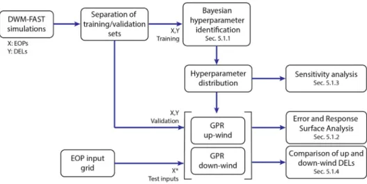
The GPR-driven numerical analysis methodology of the DWM- FAST simulations is summarized in Fig. 8. First, the GPR hyper- parameters are identi fi ed based on the Bayesian optimization method facilitated by Metropolis-Hastings sampling. The obtained hyperparameter distribution is then used to perform sensitivity analysis, while expected values are employed to perform pre- dictions used for construction of response surfaces and comparison of DELs in up-wind and wake-affected WTs.

5.1.1. Hyperparameter identi fi cation

The Bayesian inference approach based on the Metropolis- Hastings (MH) sampling algorithm described in Section 4.3, is used to estimate of the posterior hyperparameter distribution of the GPR predictor based on the available coupled DWM-FAST simulations. To this end, 180 input-output pairs are randomly selected to calculate the GPR ’ s marginal likelihood (Eq. (13)) within the MH sampling loop, while the remaining ones are used for posterior model validation. To ensure even distribution of the training samples, a sampling approach based on clustering of the complete set of inputs is performed. More precisely, an agglomer- ative hierarchical clustering tree based on Ward ’ s linkage on the Euclidean distance is applied. Subsequently, 180 clusters are built based on the obtained linkage and a single input and its respective output are randomly extracted from each one of them.

Independent log-normal distributions are de fi ned for each one of the hyperparameters. Similarly, independent log-normal distri- butions are selected as proposal distributions. The parameters of

these distributions are summarized in Table 5.

Using the previously described set-up, a total of 10 000 samples are simulated with the MH algorithm. Fig. 9 displays the distribu- tion of the GPR hyperparameters based on the sample of the hyperparameter posterior drawn with the MH algorithm, obtained with the data from the up-wind WT tower edgewise and fl apwise DELs. It is fi rst noted that although the initial values and prior distributions are similar for all the GPR hyperparameters, the posterior distributions converge to different intervals. The distri- butions for the noise variance, kernel variance and the fi rst three scale parameters ([

: wind speed; [

: turbulence intensity; [

: shear exponent) are quite narrow, [

: horizontal in fl ow skewness, has wider distributions in both edgewise and fl apwise DELs. The latter seems to indicate that the horizontal in fl ow skewness has a reduced effect in the DELs. Further analysis based on the obtained GRPs is provided in the sequel.

5.1.2. Analysis of DELs based on the obtained GPRs

5.1.2.1. Response surfaces. After estimation of the hyperparameter posterior, it is possible to calculate response surfaces of the DEL for any values in the input space. For instance, 1D slices displaying the DEL as a function of single input variables while the remaining ones are kept fi xed can be calculated with the help of the obtained GPR.

Figs. 10 and 11 display slices of the DEL in the blade e edgewise and fl apwise directione extracted from the GPR with Maximum A Pos- teriori (MAP) hyperparameter estimates on the up-wind and down- wind WTs. On each frame, the remaining inputs are set to the sample median values, while the spacing between WTs is 11 rotor diameters, and the W€ ohler exponent is m ¼ 9. In both cases, the GPR predictive mean is similar in both the up-wind and wake- affected WTs, while a signi fi cant decrement is found in the DEL of the wake-affected WT at high wind speeds. On the other hand, the con fi dence intervals are well con fi ned around the mid-part of the input range, while the dispersion increases towards the boundaries of the input ranges. The increased dispersion is observed due to the reduced number of points towards the boundaries.

Fig. 12 shows the GPR predictive mean of the DEL in the blade fl apwise direction as a function of wind speed and turbulence in- tensity ( a ^and J set to their median values, d ¼ 11, and m ¼ 9). DEL estimates with variance higher than 50 times the minimum pre- dictive variance are censored in the displayed surfaces. As observed in Fig. 11, the DEL in the blade fl apwise direction increases as the wind speed and the turbulence intensity do, with the wind speed making the maximum effect. The training data points, displayed as

Fig. 8.

Flowchart summarizing the GPR-based numerical analysis methodology of the DWM-FAST simulations.

no-Valencia, I. Abdallah and E. Chatzi Renewable Energy 170 (2021) 539e561

red dots in the surface, coincide with the GPR predictive mean, but also are con fi ned to the non-censored area, which indicates that the predictive variance is well-bounded around the area spanned by the training points. In practice, DEL estimates in points outside the non-censored area can be deemed as unreliable, while at the same

time have a low probability of occurrence, according to the joint distribution of U and s ^.

5.1.2.2. Error analysis. The predictive performance of the GPR is measured in terms of the Normalized Mean Squared Error (NMSE)

Settings of the Metropolis-Hastings algorithm for sampling of the GPR hyperparameter posterior.

Hyperparameter Prior Proposal

Kernel variance s

ln s

1;10

ln s

s

s

s

Kernel scaling

1;…;4

ln[

ln[

Noise variance

s

ln s

1;10

ln s

s

s

s

Number of Monte-Carlo samples 10

. The symbols

s

,

, and

s

indicate the values of the same quantity drawn in the previous iteration of the MH sampling algorithm.

Fig. 9.

Boxplots displaying the distribution of the GPR hyperparameters sampled with the MH algorithm for the DELs in the blade edgewise and

ohler exponent: 9.

Fig. 10.

Slices of the DEL predictive mean and 99% confidence intervals (CI) based on a GPR with MAP hyperparameter estimates obtained on the blade in the edgewise direction in the up-wind and down-wind WTs. Other inputs are kept at their training set sample median values indicated on each frame. WT spacing: 11 diameters; W€ ohler exponent: 9.

no-Valencia, I. Abdallah and E. Chatzi Renewable Energy 170 (2021) 539e561

calculated on the validation set. The NMSE is de fi ned as:

NMSE ¼ P _N

i¼1 ðy _i fðx i ÞÞ ² P _N

i¼1 y ² _i (24)

where N

is the number of samples in the validation set. Fig. 13 displays the NMSE obtained on the prediction of the DELs in the blade and tower on the up-wind and wake-affected WTs, with the wake-affected WT located at 11 rotor diameters. The error fi gures in all the cases are quite low, indicating a fair predictability in all cases, while the performance in the up-wind and wake-affected WTs is similar. In the worst case, corresponding to the tower side-to-side loads, the NMSE is under 3%. On the other hand, the best case, corresponding to the blade fl apwise loads, the NMSE is about two levels of magnitude lower than that in the tower side-to-side loads.

For the blade loads, the NMSE appears to mildly increase with the W€ ohler exponent. This tendency is followed by both up-wind and down-wind WTs.

Fig. 14 displays the NMSE as a function of the spacing between WTs for the blade and tower loads in the wake-affected WT. The overall error performance does not evidence large variations at different spacing to the values observed in Fig. 13. Moreover, the magnitude order of the NMSE is the same as that found in the previous analysis.

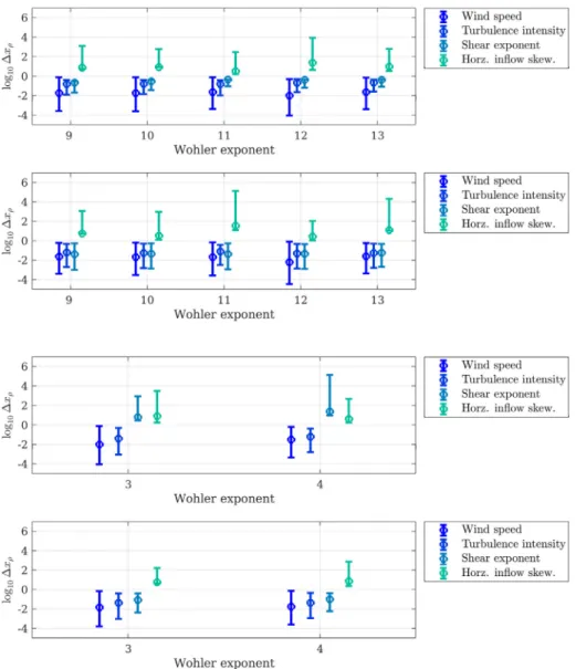
5.1.3. Sensitivity analysis based on the GPR hyperparameters A sensitivity analysis based on the increment method, described in Section 4.4, is performed on the hyperparameter sample ob- tained from the GPR hyperparameter posterior with the MH sam- pling algorithm. Fig. 15 displays the log-increments obtained for the DELs of different components in the up-wind WT as a function of the W€ ohler exponent for a correlation reduction of r ^{¼ 0} : 001. The top frame of Fig. 15 displays the log-increments obtained in the case of the loads in the blade edgewise direction. According to the re- sults, the wind speed requires the lowest variation to perform a change in the DEL, with the turbulence intensity and shear

Slices of the DEL predictive mean and 99% confidence intervals (CI) based on a GPR with MAP hyperparameter estimates obtained on the blade in the

the up-wind and down-wind WTs. Other inputs are kept at their training set sample median values indicated on each frame. WT spacing: 11 diameters; W€ ohler exponent: 9.

Fig. 12.

Surface displaying the GPR predictive mean of the DEL in the blade

direction as a function of wind speed and turbulence intensity, with the shear expo- nent and horizontal inflow skewness set on their median values. W€ ohler exponent: 9.

Red dots indicate input/output data points.

no-Valencia, I. Abdallah and E. Chatzi Renewable Energy 170 (2021) 539e561

exponent following in ranking. On the other hand, the horizontal in fl ow skewness has a much lesser in fl uence on the variation of the DELs. Considering that the range of the variables is normalized to the range ½0 ; 1, then the horizontal in fl ow skewness turns out to be inconspicuous in the DELs. This result can be contrasted with the response slices displayed in Fig. 10 for the wind turbine in the up- wind position. In effect, the wind speed seems to have the most complex in fl uence in the DELs, with the turbulence intensity and shear exponent introducing a less complex and almost linear variation, while the horizontal in fl ow skewness seems to have a

very reduced in fl uence in the DELs. On the other hand, contrasting the increments obtained for different W€ ohler exponents, it appears that this variable makes no difference on the sensitivity of DELs to input variables.

A similar interpretation can be provided for the loads in the blade fl apwise direction, and in the tower side-to-side and fore-aft directions. In the case of the blade fl apwise direction and tower fore-aft direction, the DELs are also sensitive to wind speed, tur- bulence and shear exponent, while insensitive to the horizontal in fl ow skewness. In contrast, the loads in the tower side-to-side

NMSE obtained on the prediction of different DELs on the up-wind and wake-affected WTs based on the GPR with MAP hyperparameters for different W€ ohler exponents.

Wake-affected WT located at 11 rotor diameters. Top left: blade edgewise; top right: blade

Fig. 14.

Median NMSE averaged among W€ ohler exponents as a function of the spacing between WTs in the wake-affected WT based on the GPR with MAP hyperparameters. Top left: blade edgewise; top right: blade

no-Valencia, I. Abdallah and E. Chatzi Renewable Energy 170 (2021) 539e561

direction are insensitive to both the shear exponent and horizontal in fl ow skewness. In all cases, the W€ ohler exponent has no in fl uence on the sensitivity of the DELs to input variables.

With increasing wind speed, the rotor RPM increases linearly below rated wind speed. This invariably results in increased num- ber of fatigue load cycles affecting the blade edgewise loads (most of which are driven by the weight of the blade), which explains the in fl uence of mean wind speed on blade edgewise DEL (more so than turbulence and shear). Similarly, the mean thrust loading in- creases with increasing mean wind speed, which directly in- fl uences the fl apwise loads. This is explained by the fact that at higher W€ ohler exponents, small variations in the mean loads have a disproportionate in fl uence on the DEL. Turbulence introduces sto- chasticity to the load ranges, while shear introduces cyclic varia- tions to the load ranges over one blade rotation, which explains their in fl uence on blade and thrust driven tower fatigue loads in the fore-aft direction (e.g. turbulence driving low cycle fatigue which is critical on welded steel components such as the tower). Further conclusion is that the results show marginal sensitivity to errors in the W€ ohler exponent.

Fig. 16 provides a similar analysis, this time on the loads of the wake-affected WT as a function of the spacing between WTs, with

the W€ ohler exponent set to m ¼ 9 in the case of the blade loads and m ¼ 3 in the case of the tower loads. For the blade edgewise di- rection loads, the spacing seems to bear no in fl uence on the sensitivity. However, it now appears that the horizontal in fl ow skewness has an effect in the DELs of the wake-affected WT measured in the blade edgewise direction. In the case of the blade fl apwise loads, the spacing between WTs seems to in fl uence the DELs, but not signi fi cantly. For the tower loads, the sensitivity to the shear exponent and horizontal in fl ow skewness appears to vary with the spacing between WTs. Particularly, for certain spacing the shear exponent has an effect on the loads while for others it does not. Finally, the effect of wind speed and turbulence intensity in the loads appears to be stable in the wake-affected WT regardless of the spacing to the up-wind WT.

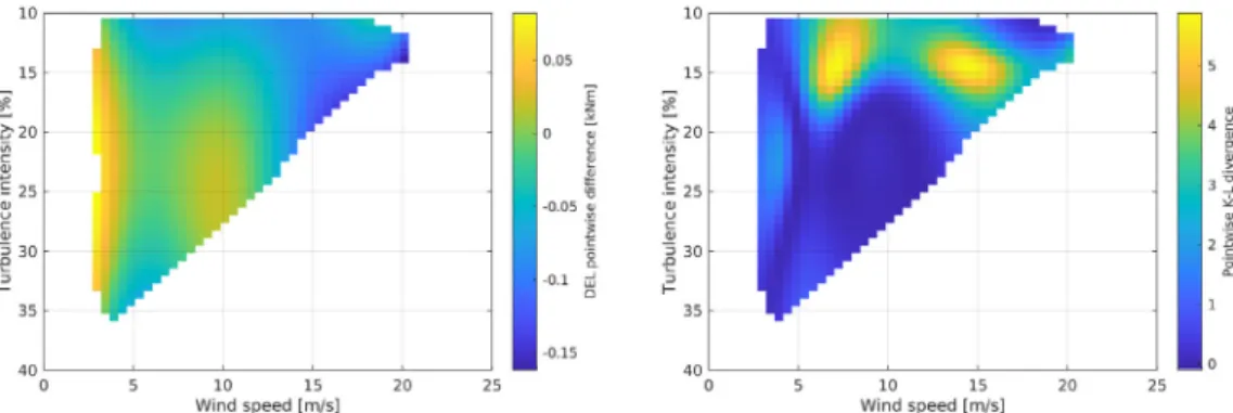
5.1.4. Comparison of up-wind and down-wind DELs

The obtained GPRs are also used to determine the difference of the loads in the up-wind and wake-affected WTs. Pointwise dif- ferences can be evaluated by directly comparing the DEL pre- dictions of the GPRs of the up-wind and down-wind WTs on a test input point x

, simply as:

Fig. 15.

Median and 90% CI of the log-increments found for each one of the input variables based on the GPR model hyperparameter sample as a function of the W€ ohler exponent for different components of the up-wind WT. From top to bottom: Blade edgewise loads, blade

no-Valencia, I. Abdallah and E. Chatzi Renewable Energy 170 (2021) 539e561