Comparison with Observations and Implications for the Dissipation Process in the Solar Wind

(1)

Turbulence with Damping by Kinetic Alfvén Waves:

Comparison with Observations and Implications for the Dissipation Process in the Solar Wind

I n a u g u r a l - D i s s e r t a t i o n

zur

Erlangung des Doktorgrades

der Mathematisch-Naturwissenschaftlichen Fakultät der Universität zu Köln

vorgelegt von Anne Schreiner

aus Daun

Köln 2017

(2)

Berichterstatter: Prof. Dr. Joachim Saur Berichterstatter: Prof. Dr. Yaping Shao

Tag der mündlichen Prüfung: 27. Juni 2017

(3)

The aim of this work is to improve the characterization of small scale processes in the solar wind, particularly, the dissipation process of the turbulent energy. Although some statistical properties of solar wind turbulence are comparable to those of hydrodynamic turbulence, the presence of the interplanetary magnetic field and the composition of the solar wind of charged particles result in important differences.

We present a dissipation model, which is based on a combination of the nonlinear energy transport from large to small scales and the damping process, which becomes important at small scales. We assume that damping is caused by interactions between kinetic Alfvén waves (KAW) and solar wind particles. The first part of this thesis presents a one-dimensional model in wavenumber space, which is compared with solar wind observations. With the help of this model, the following conclusions can be drawn about the dissipation process: assuming an anisotropic energy transport, which follows the critical balance theory, the background turbulence is driven by KAWs and not by whistler waves. This KAW driven cascade results in a quasi- exponentially shaped dissipation range and a dissipation length which corresponds to the electron gyroradius. The model provides an answer to the question as to why the dissipation length in the solar wind is independent of the energy injected at large scales, which is a clear difference compared to hydrodynamic turbulence. The anisotropic nature of the solar wind turbulence influences the transport of energy in such a way that the damping becomes more effective with a larger amount of injected energy. The expansion of the one-dimensional dissipation model to three dimensions and the thereon based calculation of reduced power spectra in the frequency space lead to the following conclusions: Damping due to KAW is able to explain the steep spectral index in the sub-ion range, which is observed in the solar wind plasma but could not be explained by any theory. However, a direct comparison with a set of solar wind observations shows that the spectral index is still steeper in the observations than the spectral index in the model. We conclude that the KAW driven cascade is present in all the observed spectra, but that other effects or wave modes can additionally influence the slope.

(4)

Zusammenfassung

Das Ziel dieser Arbeit ist es, die kleinskaligen Prozesse und insbesondere die Dissipa- tion turbulenter Energie im Sonnenwind Plasma zu charakterisieren. Obwohl einige statistische Eigenschaften der Sonnenwind Turbulenz vergleichbar sind mit denen hydrodynamischer Turbulenz, resultieren die Anwesenheit des interplanetaren Ma- gnetfeldes und die Zusammensetzung des Sonnenwindes aus geladenen Teilchen in deutlichen Unterschieden. Wir präsentieren ein Dissipationsmodell, welches auf einer Kombination aus nicht-linearem Energie Transport von großen zu kleinen Skalen und dem Dämpfungsprozess, der auf kleinen Skalen einsetzt, basiert. Es wird angenom- men, dass die Dämpfung durch Interaktionen zwischen kinetischen Alfvén Wellen (KAW) und den Sonnenwind Teilchen hervorgerufen wird. Der erste Teil dieser Ar- beit präsentiert ein eindimensionales Modell im Wellenzahl-Raum, welches mit Son- nenwind Beobachtungen verglichen wird. Mit Hilfe dieses Modells können folgende Rückschlüsse auf den Dissipationsprozess gezogen werden: Unter der Annahme eines anisotropen Enegietransports, welcher der Critical Balance Theorie folgt, wird die Hintergrund Turbulenz von KAW und nicht von Whistler Wellen getrieben. Diese KAW Kaskade resultiert in einem quasi-exponentiell geformten Dissipationsbereich und einer Dissipationslänge, die dem Elektronen Gyroradius entspricht. Das Modell gibt eine Antwort auf die Frage, warum die Dissipationslänge im Sonnenwind unab- hängig von der Energie ist, die auf großen Skalen injiziert wird, was einen deutlichen Unterschied im Vergleich zu hydrodynamischer Turbulenz darstellt. Die anisotrope Natur der Sonnenwind Turbulenz beeinflusst den Energietransport in der Art, dass bei einer größeren Menge an injizierter Energie die Dämpfung effektiver wird. Die Erweiterung des eindimensionalen Dissipationsmodells auf drei Dimensionen und die darauf basierende Berechnung reduzierter Energiespektren im Frequenz-Raum führt zu folgenden Rückschlüssen: Die Dämpfung aufgrund von KAW ist in der Lage, den steilen spektralen Index im Bereich zwischen Ionen und Elektronen Skalen zu erklären, welcher im Sonnenwind Plasma beobachtet wird, aber bisher durch keine Theorie erklärt werden konnte. Allerdings zeigt sich im direkten Vergleich mit einem Set aus Sonnenwind Beobachtungen, dass der spektrale Index in den Beobachtungen weiterhin steiler ist als der spektrale Index im Modell. Wir schließen daraus, dass die KAW getriebene Kaskade in allen beobachteten Spektren anwesend ist, dass allerdings andere Effekte oder Wellenmoden die Steigung zusätzlich beeinflussen können.

(5)

1 Introduction 1 2 Turbulence Theory and Observations of Solar Wind Turbulence 7

2.1 Hydrodynamic Turbulence and Dissipation . . . 7

2.2 Turbulence and Dissipation in the Solar Wind Plasma . . . 12

2.2.1 MHD Description of Plasma Turbulence . . . 12

2.2.2 Dispersion Relation of Kinetic Alfvén Waves . . . 16

2.2.3 Observational Evidence of Turbulence and Associated Theories 20 3 One-Dimensional Dissipation Model in Wavenumber Space 37 3.1 Idea and Derivation of the One-Dimensional Dissipation Model . . . . 37

3.2 Damping Rates of Kinetic Alfvén Waves . . . 43

3.3 Theoretical Implications for the Solar Wind Dissipation Process . . . 46

3.4 Comparison with Solar Wind Observations . . . 52

3.4.1 Comparison with Exemplary Magnetic Power Spectrum . . . . 52

3.4.2 Statistical Analysis . . . 54

3.5 Discussion . . . 56

4 Model for Reduced Power Spectra in Frequency Space 61 4.1 Calculation of Reduced Power Spectra . . . 61

4.2 Extension of One-Dimensional Dissipation Model to Three Dimensions 65 4.3 Comparison with Solar Wind Observations . . . 72

4.3.1 Data Set . . . 72

4.3.2 Calculation of Reduced Power Spectra . . . 74

4.3.3 Comparison with Exemplary Data Intervals and Analysis of the Spectral Index . . . 76

4.4 Discussion . . . 83

5 Summary and Conclusions 87

(6)

Contents

A Appendix 91

A.1 All 93 Observed Solar Wind Spectra . . . 91 A.2 Modeled Power Spectral Densities for Different Energy Distributions . 103

List of Figures 105

Bibliography 113

(7)

The word turbulence describes a phenomenon of fluid dynamics where eddies of all sizes interact nonlinearly with each other resulting in chaotic and unpredictable flows. Characteristic features of turbulent flows are a self-similar behavior of eddies at all scales, non predictable spatial temporal trajectories of single particles and extremely sensitive dependencies on initial and boundary conditions. A particular feature of turbulence is that it transports energy loss-free from large scales, where the energy is injected, up to the smallest scales, where dissipation becomes effective and transfers the energy into particle heating. Although turbulence can be observed and experienced in our every-day life going from the milk in your cup of coffee to large scale turbulence in the oceans and the Earth’s atmosphere, a complete description of turbulence remains one of the unsolved problems in physics.

The difficulty in predicting turbulent flows arises due to the fact that the Navier- Stokes equation, which is the governing equation of fluid motions, can not be solved in general but only for a few particular initial and boundary conditions. However, a statistical description of turbulence without prediction of single trajectories but statistical properties is able to help better understand the evolution of turbulence.

The first statistical theory of turbulence was proposed by Andrey Kolmogorov in 1941 (Kolmogorov, 1941a,b,c,d). The two main concepts of this work are that the eddies interact only locally¹and that the whole amount of injected energy at large scales will be dissipated into heat eventually at the dissipation scale. With the help of these two concepts in combination with scaling analysis, one can derive the characteristic scaling of the one-dimensional velocity power spectrumE(k)∝k^−5/3, which is a universal feature of hydrodynamic turbulence.

The problem of describing turbulent flows gets even more complicated when we look at magnetized plasmas, which appear in astrophysical environments such as the interstellar medium, the solar wind, or planetary magnetospheres. In these environments, the presence of the magnetic field influences the turbulent flow enormously.

The largest laboratory to study turbulence in magnetized plasmas based on in situ

1Note that the term ‘local’ refers to scales and not to positions.

(8)

1 Introduction

measurements of the magnetic and electric field and the plasma parameters that we have up to now is the solar wind. The solar wind is a steady stream of low density plasma released from the Sun’s corona filling the whole interplanetary space up to the heliopause, which is the boundary of solar wind and the interstellar medium.

The solar wind consists mainly of electrons, protons, and a smaller part of alpha particles and heavier ions. Since the first spacecrafts set out for their journey to the planets of our solar system in the early 1970s, in situ measurements of the solar wind took place and served as basis for the first studies of solar wind turbulence.

It became clear that the solar wind develops turbulent features similar to hydrodynamic turbulence with the characteristic slope of -5/3 for magnetic fluctuations in the inertial range. Most studies back than and now analyze turbulent properties based on magnetic field fluctuations because the magnetic field can be measured with higher time resolution and higher accuracy compared to the other turbulent fields. Therefore, the theoretical description of solar wind turbulence in this thesis will also be restricted to magnetic field fluctuations.

Although magnetic fluctuations in the solar wind show, in a statistical sense, a similar behavior to hydrodynamic fluctuations, three main differences occur when looking at plasma turbulence. First, the solar wind consists of charged particles which bring different characteristic scales into the system such as the gyrofrequency, the gyroradius or the inertial length of both protons and electrons, whereas the dissipation scale is the only characteristic scale in a hydrodynamic flow. Second, fluctuations of the magnetic fields are dissipated by a different mechanism than the viscosity in hydrodynamic turbulence, namely the resistivity. Owing to the extremely low resistivity, and viscosity when looking at the velocity fluctuations, of the solar wind plasma, classical mechanisms for dissipation and heating are ruled out leading to the outstanding problem how the turbulent energy is dissipated in the solar wind. The third difference of solar wind turbulence is the presence of the magnetic field which establishes a preferred direction, which results in different dynamics in the parallel and perpendicular direction with respect to the magnetic field. In addition, the magnetic field with its magnetic pressure and magnetic tension gives rise to new wave modes, namely the magnetosonic waves and the Alfvén wave, respectively. The latter modifies the turbulent nature of plasma turbulence

(9)

waves. Together, the magnetic field and the Alfvénic nature of fluctuations result in the anisotropy of plasma turbulence, which implies that the turbulent energy is transferred more rapidly to smaller perpendicular scales than to smaller parallel scales.

However, despite these remarkable differences, the self-similar behavior of magnetic fluctuations in the inertial range indicates that the qualitative picture of plasma turbulence is comparable to that of hydrodynamic turbulence, at least at scales where the MHD approximation is valid. In the inertial range, the considered scales are much larger than the characteristic plasma length scales and the wave frequencies are much smaller than the characteristic frequencies; therefore, a fluid description in the framework of magnetohydrodynamics is possible. It is well established that nonlinear interactions of Alfvén waves lead to the formation of the turbulent energy cascade to smaller scales. In this MHD limit, the scales can be seen as the diameter of an eddy which interacts nonlinearly with other eddies, analogously to hydrodynamic turbulence. Thus, it is no surprise that magnetic field fluctuations show the same spectral index of 5/3 as hydrodynamic spectra.

At scales comparable to the ion scales, namely the ion gyroradius and the ion inertial length, the MHD approximation breaks down and it becomes necessary to apply a kinetic description for the dynamics of the ions and electrons. These scales are usually referred to as the kinetic range of solar wind turbulence. In the past decade, high time resolution magnetic field measurements taken by spacecraft such as ACE, Cluster, or ARTEMIS led to a flurry of research activity to determine the characteristics of kinetic scale processes. But despite the growing number of observed data sets, there is still insufficient information to fully establish the properties of electron scale processes. Additionally, due to the requirement for a kinetic description at these scales, the interpretation of observations with the help of simulations and theoretical considerations remains particularly difficult. Therefore, a number of fundamental physical aspects of small-scale solar wind turbulence are still poorly understood. Improved characterization of these small-scale processes, especially the dissipation and heating mechanism, could give answers to outstanding questions such as how the solar corona is heated and how the solar wind is heated

(10)

1 Introduction

and accelerated.

A widely accepted picture of what happens to the turbulent energy at kinetic scales can be described as follows: When the energy reaches scales comparable to the ion gyroradius, the Alfvén wave undergoes a transition to the dispersive kinetic Alfvén wave (KAW), which generates another turbulent cascade down to the electron scales. In the vicinity of the electron gyroradius or the electron inertial length, the KAW is subject to strong Landau damping via wave-particle interactions (e.g., Howes et al., 2006; Schekochihin et al., 2009; Sahraoui et al., 2009). However, since the properties of the whistler wave, another prominent candidate for damping of turbulent fluctuations via wave-particle interactions, are similar to those of the KAW, it is difficult to distinguish these waves in observations. Hence, there is still an ongoing debate whether the small-scale fluctuations consist of whistler waves or KAWs. An- other open question is whether the turbulent cascade and the dissipation mechanism is as universal as in hydrodynamic turbulence, where a flow with the same Reynolds number and the same amount of injected energy results in the same power spectrum and where the turbulent energy is dissipated at a universal dissipation scale. In the case of solar wind turbulence, one could speculate that the behavior of turbulent fluctuations depends strongly on the current plasma parameters. Please note that similar to common terminology in the literature, the term ‘dissipation’ refers in this thesis to the transfer of energy from the magnetic field into perturbations of the particle distribution function via wave–particle interactions. The final transfer of this non-thermal free energy in the distribution function to thermal energy, i.e., the irreversible thermodynamic heating of the plasma, can only be achieved by collisions (Schekochihin et al., 2009; Howes, 2015; Schekochihin et al., 2016).

In this thesis, we focus on the description and analysis of kinetic range turbulence, especially on the dissipation processes at the smallest observed scales, the electron scales. In order to constrain the underlying physical mechanism of dissipation, we present a one-dimensional ‘quasi’-analytical dissipation model in wavenumber-space, which describes magnetic power spectra at kinetic scales. Our model combines the energy transport from large to small scales and collisionless damping, which re- moves energy from the magnetic fluctuations in the kinetic regime. We assume wave–particle interactions of kinetic Alfvén waves to be the main damping process.

(11)

plasma dispersion relation for waves in magnetized plasmas. A problem in comparing the one-dimensional spectrum in wavenumber space to observed power spectra arises when the field-to-flow angle between magnetic field and the solar wind direction is less than90°. In this case different wavevectors map to the power spectrum at a certain frequency. To overcome this problem, we extend the one-dimensional model to three dimensions and use a forward modeling approach by von Papen &

Saur (2015) to calculate reduced power spectra in frequency space, which can be compared directly with measurements. By doing so, we analyze the question whether KAW damping at electron scales can explain the sub-ion range of magnetic fluctuations, which is steeper than a theoretical description of KAW turbulence without damping predicts.

In order to create a theoretical basis for the studies in this thesis, we present relevant theories concerning solar wind turbulence and dissipation in more detail in Chapter 2. Additionally, linear theory of dispersion relations and the corresponding plasma wave modes will be presented. In Chapter 3, we describe the general idea and derivation of the one-dimensional dissipation model, show theoretical implications for the dissipation process that arise from our theoretical description, and compare the model to observed power spectra at electron scales. The results indicate that solar wind turbulence develops a universal character in a way that the electron gyroradius acts as a universal dissipation scale independently of the amount of injected energy at large scales, which is a remarkable difference compared to hydrodynamic turbulence. Part of this chapter has already been published in Schreiner & Saur (2017). In Chapter 4, we present the extension to three dimensions and the idea of the forward modeling approach, as well as comparisons of the reduced power spectra with a set of solar wind observations. In general, the sampling effect, which arises due to the mapping of different wavevectors to the power spectrum at one certain frequency, in combination with KAW damping is able to explain the steep spectral index in the sub-ion range. However, additional effects, such as intermittency and other wave modes might lead to additional steepening. Finally, in Chapter 5 we summarize our findings and discuss the limitations of our approach and the resultant implications for the solar wind dissipation process.

(12)

(13)

Observations of Solar Wind Turbulence

In order to create a basis for the understanding of the main concepts of our dissipation model, we give a short introduction to hydrodynamic turbulence in the framework of Kolmogorov’s phenomenology in the next section. Turning to solar wind turbulence, we present the theory of MHD turbulence, which shows that the concepts of hydrodynamic turbulence are in a sense transferable to plasma turbulence. Following, we introduce the concept of dispersion relations for the description of plasma waves, which play a main role in understanding the turbulent energy cascade as well as the the dissipation process in the solar wind plasma. The main part of this chapter gives an overview of solar wind observations and related theories concerning primarily the dissipation process of magnetic fluctuations. Finally, we summarize outstanding questions that arise from these observations and that create the prime motivation for the derivation of our dissipation model.

2.1 Hydrodynamic Turbulence and Dissipation

As was mentioned in the Introduction, the solar wind flow develops turbulent features similarly to hydrodynamic turbulent flows. Andrey Kolmogorov’s 1941 theory has therefore been a widely used starting point for solar wind turbulence theory. As we will see in Chapter 3 and 4, Kolmogorov’s theory on the energy cascade process and the associated dissipation scale is also one of the basis concepts in our solar wind dissipation model. On this account, we present a phenomenological description of turbulence and dissipation based on Kolmogorov’s 1941 theory in this section.

The underlying equation for the description of motions of viscous fluid substances is the Navier-Stokes equation, which principally allows a mathematical description

(14)

2 Turbulence Theory and Observations of Solar Wind Turbulence

of turbulent motions. The Navier-Stokes equation for an incompressible fluid can be written as

∂v

∂t +v· ∇v=−1

ρ∇p+ν∆v+F, (2.1)

∇ ·v= 0, (2.2)

wherevdefines the fluid velocity,ρthe mass density,pthe pressure,ν the kinematic viscosity, andFexternal forces. Here and in all following equations, upright boldface letters represent vector quantities. On the basis of the Navier-Stokes equation, a dimensionless quantity to characterize a turbulent flow, the Reynolds number Re, can be estimated by the ratio of the nonlinear termv· ∇vto the viscous termν∆v,

Re = v· ∇v ν∆v ∼ LV

ν , (2.3)

whereL and V represent a characteristic length scale and a characteristic velocity, respectively. For similar Reynolds numbers, two flows behave in a similar way independently of the actual size or velocity of the fluid. For small Reynolds numbers, a laminar flow occurs with a smooth and constant fluid motion. With increas- ing Reynolds numbers, eddies start to form, and symmetries that are given by the Navier-Stokes equation start to break. In this thesis, we will consider only high Reynolds number flows (Re1000), where the symmetries are restored in a statistical sense, which is known as fully developed turbulence.

Up to now, it has not been possible to derive a complete turbulence theory based on the Navier-Stokes equation in a deductive way. Therefore, a phenomenological theory is frequently applied to predict statistical properties of fully developed turbulence. Lewis Fry Richardson was one of the early pioneers in this research area who introduced the modern concept of an energy cascade from large to small scales and its dissipation at the smallest scales for the first time (Richardson, 1922). This idea of energy transport is called Richardson cascade, which is illustrated schematically in Figure 2.1. Here, l0 is the characteristic length scale or outer scale of the system, as it is often referred to in plasma turbulence theory, and η the dissipation scale.

With the help of these characteristic scales, the scales of the turbulent process can be

(15)

Figure 2.1: Richardson cascade of hydrodynamic turbulence. The energy is transported from large scales/large eddies to the smaller ones. Figure from Frisch (1995) p. 104.

Reproduced by permission of the Camebridge University Press.

divided into three ranges: First, the energy injection range for scales l ∼ l0, where energy is injected into the system, e.g., by an obstacle in the flow.² Second, the inertial range on scalesl with l0 lη, where the energy is transported loss-free from large to small scales; and third, the dissipation range for scales l ∼ η, where dissipation due to viscosity becomes effective and the turbulent energy is converted to heat.

Based on Richardson’s ideas of energy transport, Kolmogorov developed his fa- mous 1941 phenomenological theory. This theory is presented here very briefly following Frisch (1995), who revisited Kolmogorov’s theory in the light of newly developed theories and observations. The schematic picture of energy transport shown in Figure 2.1 brings out the two main assumptions of Kolmogorov’s phenomenology:

First, the self-similarity of eddies at all scales within the inertial range. One exam- ple of phenomenon in turbulent motions which is not self-similar is intermittency, which would result in eddies that are less and less space-filling with decreasing scale.

Second, the localness of interactions which implies that only eddies of similar size interact with each other. Under these assumptions, Kolmogorov’s 1941 theory can

2Within this phenomenological description and in the remainder of this thesis, the symbol ∼ means equal apart from constant factors on the order of unity.

(16)

be described as follows. At the energy injection scalel0, eddies with diameterd∼l0

are generated and start to decompose into smaller eddies. Eddies at scale l, with l between the injection scale l0 and the dissipation scale η, have a characteristic velocityvl, which is defined as the root-mean-square (rms) value of the velocity in a bandpass filtered interval around the wavenumberl⁻¹. The time, in which an eddy of size l undergoes a significant distortion, or in simple terms, in which one eddy decomposes into two smaller eddies, is referred to as the ‘eddy turnover time’,

tl∼ l vl

. (2.4)

In the picture of eddy decomposition, tl is also the time in which the energy is transferred from one scale to the next smaller one. Therefore, the energy flux Πl

from one scalel to smaller scales can be estimated by Πl ∼ v_l²

tl ∼ε. (2.5)

Owing to the constant flux of energy without direct energy injection or dissipation in the inertial range, the energy flux is independent of scalel and equal to the mean energy dissipation rate ε. Insertion of (2.4) into (2.5) results in

vl ∼ε^1/3l^1/3. (2.6)

The one-dimensional power spectrumEk(k)as a function of the wavenumberk ∼l⁻¹ is related to the mean kinetic energy1/2hv²i via

1 2hv²i=

Z ∞ 0

Ek(k)dk. (2.7)

With (2.6) and dimensional analysis of (2.7), the power spectrum can be written as

Ek(k)∼ε^2/3k^−5/3. (2.8)

Relation (2.8) reveals that the power spectrum follows a power-law k^−κ with a characteristic spectral indexκ = 5/3, which is often referred to as the Kolmogorov

(17)

spectral index. The existence of this power-law in the inertial range has been widely confirmed by observations and simulations (Frisch, 1995, and references within). A more general form of relation (2.8), which describes both the inertial range and the dissipation range, is given by

Ek(k)∼ε^2/3k^−5/3F(ηk), (2.9) where F(·) is a universal dimensionless function of a dimensionless argument that tends towards the Kolmogorov constant CK for small wavenumbers and becomes effective whenηk ∼1. A review on different approaches to determine the functional form of F(·) can be found in Monin & Yaglom (1975). Kolmogorov postulated in his first hypothesis of similarity that the statistical properties of small scales are uniquely and universally determined by the kinematic viscosityν, the mean energy dissipation rate ε and the scale l. On the basis of this hypothesis in combination with dimensional analysis, the characteristic Kolmogorov dissipation scale,

η= ν³

ε 1/4

(2.10) can be derived. The dissipation scale marks the end of the inertial range, in which energy dissipation is negligible. For scales smaller than the dissipation scale, the energy input at scale l due to nonlinear interactions and the energy drain due to viscous dissipation are equal. At these scales, the turbulent energy is converted to particle heat via collisions. The presented picture of turbulent energy transport is based on the idea of decaying eddies, which transport the energy from large to small scales until the viscosity becomes effective. The next section deals with the question to what extend these ideas can be transferred to the solar wind plasma with its low viscosity and resistivity.

(18)

2.2 Turbulence and Dissipation in the Solar Wind Plasma

In the following, we present an introduction to the theory of MHD turbulence, which results in the equation of motion for a magnetized plasma in terms of Elsässer variables. Leaving the MHD framework, we describe the concept of dispersion relations for plasma waves, especially the kinetic Alfvén wave, which we assume to generate turbulence in the kinetic regime. Based on these theoretical descriptions, we give an overview of solar wind observations concerning kinetic scale turbulence and the dissipation process and theories that arise from these observations.

2.2.1 MHD Description of Plasma Turbulence

As mentioned in the previous section, hydrodynamic, i.e., non-magnetized fluids, are known to be in a fully developed turbulent state for sufficiently high Reynolds numbersRe. For a magnetized plasma, e.g., the solar wind, one can derive an anal- ogous dimensionless quantity, the magnetic Reynolds number Rm, to characterize the turbulent flow. In the following, we derive the general induction equation for the magnetic field, which we use to define the magnetic Reynolds number in a similar way as was done for the hydrodynamic Reynolds number. Combining the induction equation with the MHD equation of motion leads to an equation which is in its form similar to the Navier-Stokes equation for hydrodynamic flows.

A plasma is a gas consisting of charged particles with a quasi-neutral behavior; i.e, on average, a plasma looks electrically neutral to the outside. This quasi-neutrality is a result of having roughly the same number of positive and negative charges in a plasma. Due to their electrical charges, the particles in a plasma are coupled to the electromagnetic field, i.e, their motion is affected by the electromagnetic field. The influence of the electric fieldE and the magnetic field Bon the particle motion and vice versa is described by Maxwell’s equations,

∇ ×B =µ0j+0µ0

∂E

∂t, (2.11)

∇ ×E =−∂B

∂t, (2.12)

(19)

∇ ·B = 0, (2.13)

∇ ·E = ρc

0

, (2.14)

wherej=e(nivi−neve)is the electric current andρc=e(ni−ne)the electric charge density for singly charged ions with electron and ion number densities and velocities nsandvs, respectively³. edefines the electron charge, and0 andµ0 are the vacuum permittivity and susceptibility, respectively. Starting with Faraday’s law in (2.12), and eliminating the electric field by insertion of the generalized Ohm’s law,

j=σ0(E+v×B) (2.15)

leads to

∂B

∂t =∇ ×(v×B− j σ0

), (2.16)

with the plasma conductivity

σ0 = nee² meνc

. (2.17)

Here,me is the electron mass andνc is the collision frequency of Coulomb or neutral collisions. The displacement current 0µ0∂E/∂t in Ampère’s law in (2.11) can be dropped for slow oscillating electric fields, which is a valid assumption in a plasma as long as we do not consider electromagnetic waves. Using Ampère’s law without displacement current and∇ ·B= 0, one obtains the general induction equation for the magnetic field

∂B

∂t =∇ ×(v×B) + 1 µ0σ0

∆B. (2.18)

Thus, the magnetic field can be changed either by motion of the plasma with velocity v (first term on right hand side) or by diffusion (second term on right hand side).

Similarly to the hydrodynamic Reynolds number, the magnetic Reynolds number is defined as the ratio of the convection term ∇ ×(v×B) to the diffusion term (µ0σ0)⁻¹∆B. In simple dimensional form, the magnetic Reynolds number Rm can be written as

Rm =µ0σ0LV = LV ηm

, (2.19)

3Subscriptsstands for different species, i.e., ions or electrons.

(20)

withηm = (µ0σ0)⁻¹ being the magnetic diffusivity, andLand V again characteristic length scales and velocities, respectively. For Rm 1, the diffusion term in the induction equation can be neglected and the magnetic field is frozen-in into the flow, i.e., it moves together with the flow. Only in high magnetic Reynolds number plasma flows, turbulence is generated. For Rm ∼ 1, diffusion starts to become important and the magnetic field is no longer frozen-in into the plasma. Similar to a large viscosity in a hydrodynamic flow, a large diffusivity smooths out any local magnetic inhomogeneity resulting in a non-turbulent magnetic field. In the solar wind plasma, the magnetic Reynolds number is aboutRm ≈7×10¹⁶ (Frisch, 1995);

therefore, the assumption of fully developed turbulence should be valid at least at sufficiently large distances to the Sun (∼ 0.3 AU).

Due to the coupling of charged particles to the electromagnetic field, the Lorentz force

F=q(E+v×B), (2.20)

with particle chargeq has to be taken into account in the equation of motion

∂v

∂t +v· ∇v=−1

ρ∇p+ν∆v+q

ρ(E+v×B). (2.21) Adding up Equation (2.21) for ions and electrons with number density ns, mass ms, thermal pressure ps and velocity vs, and applying a single fluid description (n = ni = ne, ρ = n(me+mi), p = pi +pe, v = (mivi +meve)/(mi +me)), one obtains the MHD equation of motion for an incompressible plasma,

∂v

∂t +v· ∇v=−1

ρ∇p+ν∆v+ 1

ρj×B, (2.22)

∇ ·v= 0. (2.23)

Within the MHD framework, the plasma is described as a single fluid, in which the dynamics of electrons and ions do not decouple. Hence, the MHD picture is valid for frequencies that are much smaller than the gyrofrequencies Ωs = qsB0/ms of ions and electrons, and for scales that are much larger than the ion and electron gyroradius ρs = vs/Ωs. B0 is the mean magnetic field and vs = p

2kBTs/ms the thermal velocity of species s with the Boltzmann constantkB and temperature Ts.

(21)

For slow variations, i.e., when the displacement current in Ampère’s law in (2.11) can be neglected, the Lorentz force termj×B can be written as

j×B =−∇

B² 2µ0

+ 1

µ0

(B· ∇)B, (2.24)

where the first term describes the magnetic pressure pB = B²/2µ0, which simply adds to the thermal pressure, and the second term describes the magnetic tension.

By separating the magnetic field B = B0 +b into the background component B0

and fluctuationsb, and introducing the Elsässer variables z^± = v±b/√µ0ρ (first introduced by Elsässer (1950)), the equation of motion in terms of Elsässer variables can be obtained by adding up (2.18) and (2.22) with the Lorentz force term as written in (2.24),

∂z^±

∂t ∓(vA· ∇)z^±+ (z^∓· ∇)z^± =−1

ρ∇P +1

2(ν+ηm)∆z^±+1

2(ν−ηm)∆z^∓. (2.25) vA=B0/√µ0ρdefines the Alfvén velocity and ∇P =∇p+∇pB is the sum of thermal and magnetic pressure. Equation (2.25) reveals two important implications:

First, if the Elsässer variables are defined in a way thatz⁺ refers to outgoing waves and z⁻ to ingoing waves, the nonlinear term (z^∓· ∇)z^± is only effective for oppo- sitely propagating Alfvén wave packets. Second, the equation of motion for Elsässer variables is in its form similar to the hydrodynamic Navier-Stokes equation indi- cating that similar assumptions concerning the cascade and dissipation process as shown in Section 2.1 can be made in the solar wind. However, the question remains how the turbulent fluctuations are dissipated in the low viscosity and low resistivity solar wind plasma. A mechanism for dissipation that is commonly presented in the literature is damping by wave-particle interactions, by which energy can be transferred from the turbulent fluctuations into perturbations of the particle distribution function leading eventually to particle heating. These wave-particle interactions can be described within the framework of kinetic dispersion relations. Owing to the non-dispersive propagation of MHD plasma waves, dissipation processes can not be described within the framework of MHD, but a kinetic description is needed. In the next section, we present the general kinetic dispersion relation of plasma waves with

(22)

special attention to kinetic Alfvén waves, which we assume to transport the energy in the kinetic regime from large to small scales.

2.2.2 Dispersion Relation of Kinetic Alfvén Waves

For the derivation of the general dispersion relation, it is necessary to express the plasma current in terms of the electric field. One way to do so is to introduce a dielectric tensor . In the following, we linearize Maxwell’s equations by assuming B=B0+δB,E=E0+δE withB0 =const. andE0 = 0. The first order quantities are assumed to vary asexp[i(k·r−ωt)]with position vectorrand frequencyω. The symbolδ for first order quantities is dropped in the following derivation. According to the first of Maxwell’s equations in (2.11), the electric displacement D consists of the vacuum displacement plus the plasma current

∇ ×B=µ0j+0µ0

∂E

∂t =0µ0

∂D

∂t . (2.26)

Fourier transformation in time and space of (2.26) leads to D(ω,k) = E(ω,k) + i

0ωj(ω,k) =(ω,k)·E(ω,k), (2.27) with the dielectric tensor(ω,k). Together with the Fourier transformed Faraday’s law (2.12)

B= 1

ωk×E, (2.28)

(2.26) can be written as

k×(k×E) + ω²

c²·E= 0, (2.29)

wherec² = (0µ0)⁻¹ defines the speed of light. After some vector algebra, the general dispersion relation for waves in a hot plasma

k⊗k−k²1+ ω² c²

·E= 0, (2.30)

(23)

is found, which has only non-trivial solutions for det

k⊗k−k²1+ ω² c²

= 0. (2.31)

1denotes the identity matrix and⊗the tensor product. Assuming that the wavevector is in thexz plane, the dispersion relation can be written in the form

det







xx−n²_k xy xz+nkn⊥

−xy yy−n² yz

xz+nkn⊥ −yz zz −n²_⊥





= 0, (2.32)

with the parallel, perpendicular and total index of refraction nk = kkc/ω, n⊥ = k⊥c/ω and n = kω/c, respectively, where kk is the parallel wavenumber and k⊥

the perpendicular wavenumber with respect to the mean magnetic field. Equation (2.31) describes in general the propagation of linear waves with frequencyω =ω(k). To determine the solution of (2.31), one must first find the dielectric tensor .

The most general way to obtain is to make use of kinetic plasma theory. The kinetic theory describes the properties of the particle distribution function and its evolution. Hence, a kinetic description takes into account kinetic effects that are carried by single plasma components, such as gyromotions of electrons and ions.

The set of fluid equations for mass, momentum and energy conservation have to be replaced by the set of Vlasov equations for every plasma component. The Vlasov equation describes the evolution of the distribution function f in a collisionless plasma according to

∂f

∂t +v∂f

∂x+ q

m(E+v×B)∂f

∂v = 0. (2.33)

Starting from the linearization of the Vlasov equation, one can obtain the tensor elements of the dielectric tensor. The equation set of general dispersion relation and dielectric tensor obtained from the Vlasov equation is therefore often referred to as the linear Maxwell-Vlasov system. The derivation of the tensor elements involves a lengthy calculation, which we do not show here, but which can be found in Stix (1992). The tensor elements for a nonrelativistic plasma with Maxwellian distributed

(24)

electrons and protons with no zero-order drift velocities can be cast in the form (e.g., Chen, 1974; Stix, 1992; Baumjohann & Treumann, 2012)

xx = 1 +X

s

ω_ps² ω²ξ0s

∞

X

n=−∞

n²Γn(µs) µs

Z(ξns), (2.34)

yy = 1 +X

s

ω_ps² ω²ξ0s

∞

X

n=−∞

n²Γn(µs)

µs −2µsΓ⁰_n(µs)

Z(ξns), (2.35)

zz = 1−X

s

ω²_ps ω²ξ0s

∞

X

n=−∞

ξnsΓn(µs)Z⁰(ξns), (2.36)

xy = iX

s

ω_ps² ω² ξ0s

∞

X

n=−∞

Γ⁰_n(µs)nZ(ξns), (2.37)

xz = −X

s

sgn(qs)ω_ps² ω²ξ0s

∞

X

n=−∞

√1 2µs

nΓn(µs)Z⁰(ξns), (2.38)

yz = iX

s

sgn(qs)ω_ps² ω²ξ0s

∞

X

n=−∞

Γ⁰_n(µs)Z⁰(ξns) rµs

2 , (2.39)

where ωps = (nsq_s²/0ms)^1/2 is the plasma frequency of species s, Ωs = qsB/ms

is the gyrofrequency of species s (negative for electrons), ξns = (ω − nΩs)/kkvs, vs = (2kBTs/ms)^1/2 is the thermal speed of species s, andµs = 0.5k²_⊥ρ²_s with the gy- roradiusρs=vs/Ωs. The functionZ(ξ)is the plasma dispersion function, which was introduced by Fried & Conte (1961). Its derivative is given byZ⁰(ξ) =−2−2ξZ(ξ).

Γn(µs) = e^−µ^sIn(µs), where In is the modified Bessel function of the first kind of ordern. Note that the derivative of Γn is given by Γ⁰_n(µs) = (I_n⁰(µs)−In(µs))e^−µ^s. After insertion of the dielectric tensor into the general dispersion relation (2.31), one can obtain the wave frequency as a complex number ω=ωr+ iγ, whereωr describes the dispersion of the wave mode andγ its damping. The validity of applying linear theory of dispersion relations to the nonlinear turbulent energy transport is discussed in the discussion part of Chapter 3. In the limits of MHD, wave frequencies of plasma waves do not have an imaginary part. Hence, only kinetic waves can be responsible for damping of turbulent fluctuations. The most prominent candi- dates for damping presented in the literature are kinetic Alfvén waves and whistler waves, which are both extensions of the MHD Alfvén wave with dispersion relation

(25)

ωA = ±kkvA into the kinetic regime. The difference of KAW and whistler waves is

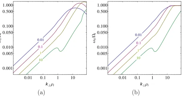
Figure 2.2:Solutionω/Ωi of linear Maxwell-Vlasov equations as a function ofkρi : Real part of wave frequency is shown in blue, damping rate γ in red for different angles of propagationθkB. The inset shows the same plot with double-logarithmic axes to illustrate the transition from non-dispersive to kinetic regime at wavenumbers ∼ kρi = 1. Figure from Sahraoui et al. (2012). Reproduced by permission of the American Astronomical Society.

shown in Figure 2.2. KAWs propagate at quasi-perpendicular propagation angles θkBwith frequenciesωKAW <Ωi, whereas whistler waves are defined as the extension of Alfvén waves with ωw ≥ Ωi. As we will show in Chapter 3, wave frequencies in the solar wind under the assumption of critical balance (a model for the anisotropy of energy transfer in the solar wind with respect to the magnetic field, which is introduced in Section 2.2.3) do not exceed the ion gyrofrequency. Therefore, we refer to the solution of the general dispersion relation in our model as KAWs. Extensions of the MHD magnetosonic modes into the kinetic regime are not considered to carry the energy down to the scales of dissipation, i.e., the electron scales, because the slow

(26)

magnetosonic mode is heavily damped at ion scales and the fast magnetosonic mode undergoes resonances at the ion gyrofrequency (Sahraoui et al., 2012). Against this background, we present observations of power spectral densities of magnetic fluctuations in the solar wind and associated theoretical descriptions in the following section.

2.2.3 Observational Evidence of Turbulence and Associated Theories

In the following, we present observations of magnetic power spectra in the solar wind going from observations at MHD and sub-ion scales to observations at electron scales. On the basis of these observations, the differences of whistler wave and KAW turbulence are introduced, as well as the concept of a critically balanced energy cascade.

Observations from MHD to Sub-Ion Scales

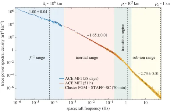
Owing to the extremely high (magnetic) Reynolds numbers of the solar wind plasma at1 AU, the turbulence is assumed to be highly developed. This turbulent state of fluctuations is evidenced by magnetic field measurements, which show very broad- band power spectral densities P(f) or P(k) illustrating the amount of energy per frequency or wavenumber, respectively (e.g., Coleman JR., 1968). This indication of the turbulent cascade is shown in Figure 2.3. We focus in this section on the magnetic power spectral density because it is the focal point of most solar wind turbulent studies, and it gives a simple overview of the scales of interest and the associated physical mechanism. Due to the high speed of the solar wind flow larger than most of the dynamics of the system, Taylor’s hypothesis (Taylor, 1938) can be applied to relate temporal and spatial scales viaf =k⊥vSW/2π with the solar wind velocity vSW. The time series measured by the spacecraft therefore corresponds to one-dimensional spatial measurements along a straight line in the plasma frame. As is shown in Chapter 4, this relation is valid only for measurements with high angles between the magnetic field and the solar wind flow direction θvB. For solar wind measurements close to Earth, where measurements with field-to-flow angles θvB of

(27)

Figure 2.3:Power spectral density of the magnetic field fluctuations for typical solar wind parameters at 1 AU. Blue and red lines are calculated from ACE measurements; yellow line from Cluster measurements. Instruments and interval lengths are given in the legend.

The vertical dashed lines indicate the correlation lengthλc, the ion gyroradiusρi, and the electron gyroradiusρ_e. Figure from Kiyani et al. (2015). Reproduced by permission of the Royal Society.

less than50° are often related to the Earth’s foreshock, and therefore not considered in the analysis of solar wind turbulence, this assumption is sufficiently fulfilled.

In Figure 2.3, four distinct regions of interest are marked by different background colors: the f⁻¹ range, the inertial range, the transition region at ion scales, and the sub-ion range. In the f⁻¹ range, the temporal variability of the Sun and its corona, the source of the solar wind, is visible (Matthaeus & Goldstein, 1986). This connection to the Sun breaks down for scales smaller (frequencies higher) than the correlation lengthλc. Hence, below this scale, the fluctuations are a product of the in situ dynamics in the solar wind flow (Kiyani et al., 2015). The correlation length also defines the size of the largest energy containing ‘eddies’ of the turbulent flow.

In the inertial range the MHD energy cascade from large to small scales takes place.

It is well established that the power spectral density follows approximately the Kol-

(28)

mogorov indexf^−5/3 in this range (e.g., Matthaeus et al., 1982; Denskat et al., 1983;

Horbury et al., 1996; Leamon et al., 1998a; Bale et al., 2005). Although the hydrodynamic phenomenology of neutral fluids can partially be transferred to inertial range plasma turbulence, additional physics of the anisotropy of the energy transport have to be taken into account, which are introduced in Section ‘Anisotropy and Critical Balance’. The inertial range ends when the turbulent energy reaches the ion scales, where the fluid picture of MHD breaks down. At these scales, the physical mechanisms change leading to a modification of the cascading process possibly including dissipation, which results in a steepening of the spectral slope (Leamon et al., 1999;

Alexandrova & Carbone, 2008; Chen et al., 2014). At scales smaller than ion scales, a second cascade range up to electron scales with a steeper slope of about -2.9 to -2.3 is observed (Alexandrova et al., 2009; Kiyani et al., 2009; Chen et al., 2010;

Sahraoui et al., 2010), which is called the sub-ion range. Between the inertial range and the sub-ion range, a transition region is observed, where the spectra exhibit a power-law with a variable spectral slope of -4 to -2 (Leamon et al., 1998a; Smith et al., 2006; Roberts et al., 2013) or a smooth non-power-law behavior (Bruno &

Trenchi, 2014).

These observations appear to be consistent with an important role of KAWs. The following picture of KAW-generated turbulent cascade is presented in the literature:

In the inertial range nonlinear interactions between Alfvén waves are responsible for the generation of the turbulent cascade. The steeping in the transition region has been associated with ion dissipation (Denskat et al., 1983; Smith et al., 2012) or with the presence of coherent structures (Lion et al., 2016). However, the process that leads to a steepening of the spectrum in the sub-ion range, i.e., between ion and electron scales, is the transformation from the non-dispersive Alfvén wave to the dispersive KAW (Howes et al., 2006). The energy in Alfvénic fluctuations generates a dispersive KAW cascade down to the electron scales, which again can be described in fluid-like terms (Schekochihin et al., 2009). Whether the kinetic scale fluctuations have the characteristics of KAW (Leamon et al., 1998b, 2000; Bale et al., 2005;

Howes et al., 2008; Schekochihin et al., 2009) or whistler waves (Stawicki et al., 2001;

Gary & Smith, 2009; Podesta et al., 2010), is still a much debated topic. Recent observations concerning this question are presented in the next section.

(29)

Whistler Waves versus Kinetic Alfvén Waves

Knowledge of the nature of kinetic fluctuations is essentially needed to unravel the physical mechanism by which the turbulent energy is dissipated at small scales.

The problem in identifying the wave mode that generates turbulent fluctuations is that it is not possible to distinguish uniquely between the fluctuations due to the sweeping of spatial structures past the spacecraft and temporal fluctuations in the plasma frame in single-point spacecraft measurements. As mentioned in Section 2.2.2, dispersion relations of KAW and whistler waves are similar, therefore, turbulent energy spectra derived from dimensional analysis are the same for both wave modes. However, two quantities that differ for KAW and whistler waves are the ratio of electric to magnetic fluctuations and the ratio of the amplitude of parallel magnetic fluctuations to perpendicular magnetic fluctuations. By calculating these properties for kinetic Alfvén waves and whistler waves and comparing them directly to spacecraft measurements, Salem et al. (2012) find that small scale fluctuations are not consistent with whistler waves. Weakness of their analysis is that they calculate the mentioned ratios based on the cold plasma dispersion relation for whistler waves and not from linear Maxwell-Vlasov theory. Due to the dependence of this approach on the chosen model for dispersion relations of KAW and whistler waves, various authors came to different conclusions (Sahraoui et al., 2012; Gary & Smith, 2009;

Smith et al., 2012; He et al., 2012; Kiyani et al., 2013).

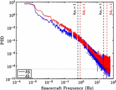
A more recent study of Chen et al. (2013) analyses small scale fluctuations based on the difference in frequencies of KAW and whistler waves. As shown in Section 2.2.2, KAWs are low-frequency waves withω Ωi, orω k⊥viat scales comparable to the ion gyroradius. Hence, the ions, along with the electrons, are fast enough to be involved in the dynamics. On the contrary, whistler waves are high-frequency waves, where ion density fluctuations, and therefore, due to quasi-neutrality also electron density fluctuations, can be neglected. Figure 2.4 shows power spectral densities of the normalized magnetic field in red and the normalized density in blue.

Between ion and electron scales, both spectra show similar amplitudes suggesting that the fluctuations consist of kinetic Alfvén waves, rather than whistler waves.

The observed mean value of δ˜n²/δ˜b²_⊥ = 0.75^+0.22_−0.17 is close to a value of 0.786±0.004 obtained in kinetic Alfvén wave simulations and much larger than the expected

(30)

Figure 2.4: Power spectral densities of the normalized magnetic field δb˜ = δB/B₀ in red and the normalized electron density δn˜ ∼ δn/n₀ in blue measured by ARTEMIS-P2 on October 11, 2010 from 00:21 to 01.14 UT. Vertical dashed lines mark ion and electron gyroradius and inertial length. Figure from Chen et al. (2013). Reproduced by permission of the American Physical Society.

value for whistler waves of ≤ 0.03. The obtained absence of whistler waves in solar wind fluctuations justifies applying Taylor’s hypothesis, which is valid for low- frequency dynamics, to relate temporal and spatial scales. Besides the question, which wave mode transports the energy to smaller scales, the answer to the question how the presence of the magnetic field influences this energy transport is crucial for understanding the dissipation mechanism.

Anisotropy and Critical Balance

In the following, we present the concept of anisotropic turbulence and the problems in analyzing the anisotropy in spacecraft measurements, followed by a brief overview of observations that show evidence of anisotropic turbulence. The presence of a local magnetic field results in a breaking of the isotropy in the properties of turbulent fluctuations as it is the case in non-magnetized fluids. The result is the existence of various anisotropies with respect to the magnetic field: First, the anisotropy of the energy transfer rate, i.e., the energy of turbulent fluctuations is transferred more

(31)

rapidly to smaller perpendicular scales than to smaller parallel scales, which results in a power anisotropy in wavevector space, which is called wavevector anisotropy (e.g., Shebalin et al., 1983; Goldreich & Sridhar, 1995). This anisotropic energy cascade leads secondly to the power anisotropy in frequency space, that is, different levels of power at a certain frequency in the spacecraft frame for different field-to- flow angles (e.g., Bieber, 1996; Horbury et al., 2008). And third, the anisotropic energy cascade results in an anisotropy of the spectral index, i.e., the scaling of the turbulent power is different for different field-to-flow angles (e.g., Horbury et al., 2008).

Difficulties in extracting information regarding these anisotropies from solar wind measurements arise due to the measurement geometry of spacecraft measurements.

The spacecraft measures the so-called reduced power spectrum (Fredricks & Coro- niti, 1976)

P(f) = Z

P(k)·δ(k·vSW −2πf)d³k, (2.40) which contains contributions of various wavevectors with different orientations and wavelengths. In order to make progress in analyzing anisotropic properties, assumptions about the underlying energy distribution in wavenumber space have to be made. In so-called ‘weak’ turbulence, the energy is transported to larger perpendicular wavenumbers, whereas the parallel wavenumber is preserved. For large wavenumbers, the power is consequently associated with wavevectors at very large field-to-flow angles, which is called ‘2D’ turbulence. This picture led to theories, that solar wind fluctuations consist of mainly ‘2D’ fluctuations combined with ‘slab’

fluctuations, where the power lies only in parallel wavevectors (e.g., Matthaeus et al., 1990; Tu & Marsch, 1993; Bieber, 1996). When the power in weak turbulent fluctuations cascades to smaller scales, the nonlinear timescale decreases, whereas the Alfvén timescale remains constant because there is no change in the parallel wavenumber. Therefore, these timescales will become equal eventually, which is called ‘strong’ turbulence. Goldreich & Sridhar (1995) proposed that this equal- ity will remain within the energy cascade to smaller scales, which is called ‘critical balance’. By equating the nonlinear timescale at which the energy is transferred to smaller scales with the linear Alfvén timescale, one finds the ratio of parallel to perpendicular wavenumbersk ∼ k^2/3 (detailed derivation of this ratio in both the

(32)

MHD and the kinetic regime is given in Chapter 3). Hence, the turbulence becomes more anisotropic for high wavenumbers, and the energy is cascaded mainly in the perpendicular direction. In the kinetic regime, where the turbulence is driven by KAWs or whistler waves, a modified critical balance can be derived, where the nonlinear timescales are equated with the linear timescales of the kinetic wave modes, which leads to a wavenumber ratio ofkk ∼k_⊥^1/3(Cho & Lazarian, 2004; Schekochihin et al., 2009). Based on critical balance, a spectral index in the inertial range of 5/3 for θvB = 90° and of 2 for θvB = 0° and in the kinetic regime of 7/3 for θvB = 90°

and of 5 forθvB = 0° (for both KAW and whistler wave driven turbulence) can be derived by dimensional analysis.

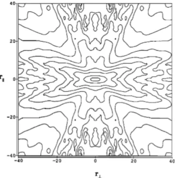
The first clear observational evidence of wavevector anisotropy is presented in Matthaeus et al. (1990), who calculated the correlation function of magnetic field fluctuations as a function of distance parallel and perpendicular to the magnetic field, which is shown in Figure 2.5. The results show that the turbulence is not consistent with a purely isotropic wavevector distribution, which would have circular contours. Evidence of the power anisotropy in the spacecraft frame in the inertial range, i.e., higher levels of power for large field-to-flow angles than for small field- to-flow angles is found in Bieber (1996), Narita et al. (2006), Horbury et al. (2008), Podesta (2009), Osman & Horbury (2009), and Luo & Wu (2010). An exemplary observation of the power anisotropy is shown in Figure 2.6 (Wicks et al., 2010).

The magnetic power spectrum obtained by Fourier transform is shown in black, the spectrum obtained by wavelet analysis for θvB = 0° (filled dots) and for θvB = 90° (filled squares) is shown in blue. The power is isotropic at large scales and becomes more and more anisotropic with decreasing scale. Additionally, Figure 2.6 reveals that the anisotropic power can only be achieved by having different scalings in different directions to the magnetic field. The observed spectral index anisotropy in the inertial range with a spectral index of 5/3 for θvB =90° and of 2 for θvB = 0°

has been commonly reported (e.g., Horbury et al., 2008; Podesta, 2009; Luo & Wu, 2010; Chen et al., 2011), when using the local magnetic field in a scale-dependent way. This scaling is in agreement with critical balance theory. In studies that take the mean magnetic field as the mean of the entire length of the observed interval, no spectral index anisotropy is seen (Tessein et al., 2009).

(33)

Figure 2.5: Contour plot of the two-dimensional correlation function as a function of distance parallel and perpendicular to the magnetic field obtained from 463 intervals of ISEE 3 magnetometer data. The original data in ther_k >0andr⊥>0quadrant has been reflected to fill all four quadrants. rk and r⊥ is shown in units of 10¹⁰cm. Figure from Matthaeus et al. (1990). Reproduced by permission of the American Geophysical Union.

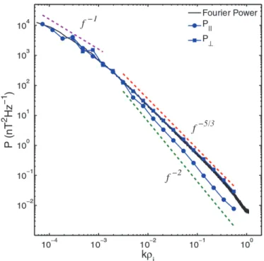
Power anisotropy in the kinetic regime was first reported by Leamon et al. (1998a), who find a lower level of anisotropy in the kinetic range than in the inertial range, whereas more recent studies by Chen et al. (2010) and Sahraoui et al. (2010), using multi-spacecraft techniques, find higher levels of anisotropy in the kinetic range, which are comparable to or even higher than the observed levels of anisotropy in the inertial range. Figure 2.7 shows the spectral index anisotropy in the kinetic regime of magnetic field fluctuations both parallel (red) and perpendicular (blue) to the local magnetic field. The spectral index for perpendicular fluctuations δB_⊥² varies from around 2.6 for large field-to-flow angles to 3.2 for small angles. The authors mention that their method of obtaining the spectral index from the second order structure function can measure spectral indices up to a value of 3. Therefore, the spectrum in the parallel direction is∼k_k⁻³ or steeper. Although the spectral indices at large field-to-flow angles are steeper than the theoretical prediction of 7/3, the

(34)

Figure 2.6:Wavelet (blue) and Fourier (black) spectrum of magnetic fluctuations obtained from Ulysses data of day 100-200 of 1995. Figure from Wicks et al. (2010). Reproduced by permission of the Oxford University Press.

steepening of the spectral index towards small angles suggests that the picture of a critically balanced energy cascade is correct. However, the observed values of δB_k² are less consistent with the theoretical predictions because δB²_k is expected to scale in the same way asδB_⊥² for a KAW energy cascade (Schekochihin et al., 2009). This result suggests that the KAW picture might be incomplete and other wave modes or cascade mechanisms might contribute to the energy transport. Although recent observations and simulations are consistent with the critical balance assumption (TenBarge & Howes, 2012; He et al., 2013; von Papen & Saur, 2015), its applicabil- ity to solar wind turbulence is still subject of debate, and other models are proposed to explain the anisotropy (Narita et al., 2010; Li et al., 2011; Horbury et al., 2012;

Wang et al., 2014; Narita, 2015).

(35)

Figure 2.7: Spectral index of magnetic power spectral densities in the kinetic regime for fluctuations parallel (red) and perpendicular (blue) with respect to the magnetic field obtained by Chen et al. (2010) from Cluster data. Figure from Chen et al. (2010). Repro- duced by permission of the American Physical Society.

Observations of Electron Scale Turbulence

The turbulent energy, which is transported in a KAW generated cascade from ion to smaller scales, finally reaches the electron scales, i.e., the electron gyroradius ρe

and the electron inertial length λe. These scales are typically ∼ 1 km in the solar wind at 1 AU (Alexandrova et al., 2009; Sahraoui et al., 2009), and hence, they are convected past the spacecraft in a couple of milliseconds at typical solar wind velocities. Therefore, observations that are able to resolve the fluctuations at these scales must be made at cadences of the order of 100 Hz, which requires high time resolved magnetic field and plasma data measurements. Although Denskat et al.

(1983) obtained high resolution magnetic spectra from Helios measurements up to 50 Hz at 1 AU and up to 470 Hz at 0.3 AU, the characteristic electron scales were not reached. It was only with the Cluster STAFF instrument, which consists of a search coil magnetometer and a spectrum analyzer instrument, that these scales were resolved for the first time.

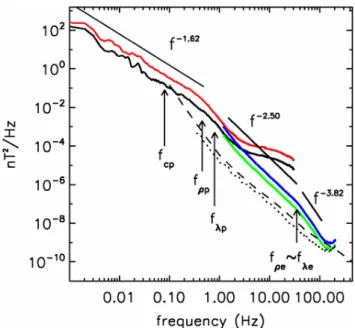
The first direct determination of the dissipation range at electron scales in solar wind turbulence is reported in Sahraoui et al. (2009); their results are shown in Fig- ure 2.8. The parallel (black, green) and perpendicular (red, blue) magnetic power spectral densities follow a power-law with a spectral index close to the Kolmogorov

(36)

Figure 2.8: Parallel (black, green) and perpendicular (red, blue) magnetic power spectral densities of Cluster FGM data up to 33 Hz and STAFF-SC data for frequencies between 1.5 Hzand225 Hzmeasured on 19 March 2006 from 20h30 to 23h20 UT. Dashed and dotted lines give the noise level, respectively. Black arrows indicate characteristic frequencies.

Figure from Sahraoui et al. (2009). Reproduced by permission of the American Physical Society.

index in the inertial range, and a power-law with a spectral index of 2.5 in the sub- ion range, which is in agreement to the observations shown in Section ‘Observations from MHD to Sub-Ion Scales’. These observations show, for the first time, that the turbulent energy cascade at ion scales continues at least for about two more decades in spacecraft frequency. This result suggests that the turbulent energy is at the most slightly damped at ion scales and undergoes another turbulent cascade down to electron scales (marked by fρe and fλe). At these scales, a second breakpoint is seen followed by a steeper spectrum of∼f^−3.8. The observation appears consistent with the KAW theory, were strong electron Landau damping at electron scales re- moves energy from the turbulent cascade, which may explain the strong steepening of the spectrum tof^−3.8. Landau damping is one kind of wave-particle interaction, where the particles gain energy from the turbulent fluctuations when the resonance conditionωr ∼kkvs is fulfilled. By equating the Landau resonance condition and an approximate KAW frequency ωr =±kkvAk⊥ρi/p

βi+ 2/(1 +Te/Ti) (Howes et al.,