Virtual fatigue diagnostics of wake-affected wind turbine via Gaussian Process Regression
Luis David Avenda˜no-Valenciaa,1, Imad Abdallahb,1, Eleni Chatzib
aDepartment of Technology and Innovation, University of Southern Denmark, Campusvej 55, 5230 Odense M, DK
bInstitute of Structural Engineering, ETH Zurich, Switzerland
Abstract
We propose a data-driven model to predict the short-term fatigue Damage Equivalent Loads (DEL) on a wake-affected wind turbine based on wind field inflow sensors and/or loads sensors deployed on an adjacent up-wind wind turbine. Gaussian Process Regression (GPR) with Bayesian hyperpa- rameters calibration is proposed to obtain a surrogate from input random variables to output DELs in the blades and towers of the up-wind and wake-affected wind turbines. A sensitivity analysis based on the hyperparameters of the GPR and Kullback-Leibler divergence is conducted to assess the effect of different input on the obtained DELs. We provide qualitative recommendations for a minimal set of necessary and sufficient input random variables to minimize the error in the DEL predictions on the wake-affected wind turbine. Extensive simulations are performed comprising different random variables, including wind speed, turbulence intensity, shear exponent and inflow horizontal skewness. Furthermore, we include random variables related to the blades lift and drag coefficients with direct impact on the rotor aerodynamic induction, which governs the evolution and transport of the meandering wake. In addition, different spacing between the wind turbines and W¨ohler exponents for calculation of DELs are considered. The maximum prediction normalized mean squared error, obtained in the tower base DELs in the fore-aft direction of the wake affected wind turbine, is less than 4%. In the case of the blade root DELs, the overall prediction error is less than 1%. The proposed scheme promotes utilization of sparse structural monitoring (loads) measurements for improving diagnostics on wake-affected turbines.
Keywords: wind turbine, fatigue, wake, uncertainty, Gaussian Process Regression, Bayesian calibration, sensitivity analysis, virtual sensing
Nomenclature
α Wind shear exponent
E Expected value of a random variable V Variance of a random variable
D Rotor diameter
Ψ Inflow horizontal skewness σ Turbulence
CD Aerodynamic drag coefficient CL Aerodynamic lift coefficient DEL Damage Equivalent Load GP R Gaussian Process Regression
mB Wh¨oler exponent for blade (composites) mT Wh¨oler exponent for tower (welded steel) M L Machine Learning
RV Random Variable
1Authors made equal contributions to the study and the publication
Ti Turbulence intensity U Mean wind speed W T Wind Turbine
1. Introduction
The load effects and degradation of structural components of wind turbines (WTs) do not uniformly evolve across a wind farm due to, largely, wake effects and variability in the inflow conditions (and waves for offshore wind farms [25]). The assessment of fatigue damage accumulation on assumption of availability of direct load effects measurements on all main structural components across all wind turbines within a wind farm is not realistic. The assumption of availability of high- fidelity aero-servo-elastic simulators of the investigated wind turbines coupled to site-specific inflow and wake models is convenient, but often not borne out of the actual reality experienced by wind farm owners and operators. At best, the designer/manufacturer of the wind turbine might make a single comprehensive one-off set of output load effects of such wind farm simulations available to the owner/operator of the wind farm.
A further and, from the view of this paper, perhaps more important hindrance lies in the precise estimation of structural response signals that are typically not available in the standard data emanating from the Supervisory Control and Data Acquisition (SCADA) monitoring systems embedded on wind turbines. A number of works therefore attempt condition monitoring on the basis of SCADA availability [47, 26]. However, when structural monitoring information becomes available [16], then this can be exploited as a more direct proxy to diagnose sudden damage [8], or to further accurately assess the remaining useful lifetime of a wind turbine in a given wind farm [17, 19, 33, 44]. We therefore posit that considerable improvements to the operation, maintenance and prediction of remaining useful life of a wind turbine can be accomplished by delivering access to transparent, simple, yet powerful and interpretable data-driven predictive models. Such models could be trained, tuned and updated via (fairly) easily accessible and cheap structural response observations from a limited number of appropriately selected wind turbines in a given wind farm [31].
The work presented herein focuses on the effects induced by wakes on the Damage Equivalent Loads (DELs) on structural components of WTs. The fatigue load variation within an offshore wind farm is primarily a product of wake-induced flow disturbances [42]. The form and severity of the wake-induced turbulence and deficit depend on multiple factors, which are in this work grouped into three classes:(a) ambient conditions (wind speed, ambient turbulence, atmospheric stability, wave height, and others);(b) wind turbine operational regime (rotor thrust, rotational speed, and power set point); and (c) relative position of the wake source(s) with respect to the disturbed turbine.
Recent literature has attempted to tackle the fatigue variability issue, by delivering predictive frameworks that capitalize on availability of SCADA data. The approaches in delivering such predictive models may be distinguished in terms of two main categories, namely the physics-based and data-driven classes.
Initiating from a physics-based approach, research in [12] and in similar works [41,37] exploits a surrogate approach, relying on Polynomial Chaos Expansions (PCE) and Artificial Neural networks (ANN), trained on pre-simulated load scenarios, to predict the fatigue load variation on WTs for a wind farm with arbitrary layout under wake effects. ANNs are shown to outperform PCE in terms of prediction accuracy and computational speed [40], albeit being prone to overfitting, while further require significantly more data for achieving acceptable performance. Both methods allow for obtaining analytical derivatives, which is a useful trait in optimization and sensitivity analysis. In [11] the performance of five surrogate models is assessed by comparing site-specific lifetime fatigue load predictions at 10 sites using an aeroelastic model of an individual DTU 10MW reference wind turbine. The compared methods include PCE, quadratic response surface, universal Kriging, importance sampling, and nearest-neighbor interpolation. The authors argue that PCE-based (and Kriging) models may sometimes have a practical advantage over ANNs, due to the “white-box”
features – such as being able to track separate contributions to variance (and uncertainty). Research in [15] proposed a procedure for producing a lifetime fatigue load variation map within an offshore wind farm. Factors such as ten-minute average free wind speed, free wind direction, ambient turbulence, farm layout and wake effects, wave height, peak period, and alignment with the wind were considered. The procedure relies on direct aero-elastic simulations of the whole wind farm including wake effects using the DWM model. A similar approach was adopted in the work of Tagliatti [43]. This mapping is not directly extendable for use with continuous and long-term structural health monitoring data (SHM).
In a purely data-driven scheme, which does not take aeroelastic analyses into account, Pap- atheou et al. [34] focus on power prediction for the Lillgrund wind farm [2] for the purpose of condition monitoring and fault detection. They adopt both ANNs and Gaussian Processes (GPs) for producing individual and population-based power curves. They then attempt prediction of the power produced on individual WTs based on measurements extracted from other turbines in the farm. A comparison between neural networks and GPs reveals no significant difference in terms of precision, but showcases the inherent ability of the GPs to produce probabilistic bounds. Woo
et al. [46] propose a Multi-Tasks Convolutional Long Short-Term Memory Network approach to simultaneously predict the energy output and structural load from the target wind turbine, while modeling the spatio-temporal structure of the input wind flow. The work is verified on simulations from a stand-alone NREL-5MW onshore reference wind turbine. The predictions are delivered in a short-term horizon, i.e., few seconds ahead. In both [34,46] wake effects are not considered. Wake is tackled in [32], where a trained Variational Autoencoder (VAE) is exploited to map the high dimensional correlated stochastic variables over the wind-farm, such as power production and wind speed, to a parametric probability distribution of much lower dimensionality, with the ultimate goal of condition monitoring.
In a method that attempts to fuse physics-based simulators with data, in what concerns the train- ing of predictive ML models, Dimitrov et al. [13] propose to use a combination of limited SCADA based measurements and wind turbine/farm simulations. An artificial intelligence framework is trained to forecast the future performance of the wind turbine and the fatigue life consumption of its components. If SCADA measurements, such as measured power production, wind speed and rotor speed, are available, the load mapping can be realized by training a data-driven regression model using e.g. artificial neural networks (ANN). In the absence of actual loads data, an aeroelastic model of the turbine can be used to generate a synthetic data set to serve for training. A com- parison of the normalized damage equivalent blade root flap moments between measurements and simulations shows a discrepancy of the order of 10%−15% for some of the operating wind speeds.
Park & Park [35] present an attempt to fuse data with engineering principles via a physics-induced graph neural network (PGNN) model able to estimate the power outputs of all wind turbines in any layout under any wind conditions. An engineering wake interaction model serves as a basis function, which effectively imposes physics-induced bias for modelling the interaction among wind turbines into the network structure. To clearly understand the role of the physics-induced weight function, the authors compare the PGNN performances to a purely data-induced approach, termed data-induced GNN (DGNN). When a target turbine in a wind farm experiences more complex wake interaction, the DGNN tends to overestimate power generations. A drawback of the proposed method is the inability to produce probabilistic output.
The overview of existing literature reveals that, on the one hand, deep learning (DL) neural network based methods (Recurrent, Convolution, GraphNets, Auto-encoders, etc.) are suited to the problem at hand, but require special understanding and tuning of the network layers to reach adequate predictive results. Moreover, these often require large training datasets in order to avoid over-fitting. Despite significant advancements in this field, DL methods remain black-box in their very nature and comprehensive interpretable results remain difficult (for now). A number of surro- gate approaches are proposed but are focused on offering an emulator of the load responses across wind turbines in a wind farm based on pre-compiled aeroelastic simulations. A lack is noted with respect to comprehensive efforts for predicting wake-induced load effects on WTs. An important goal would be to predict the loads on unmeasured wake-affected WTs via direct input loads and inflow measurements extracted from wake-free wind turbines in the same farm. This problem is particularly relevant in a realistic SHM setting for wind farms, since an efficient monitoring scheme, should involve carefully planned and, to the degree possible, sparse structural measurements.
In this work, we propose adoption of classical Gaussian process Regression (GPR) with Bayesian learning of hyper-parameters. We argue that GPR offers a number of advantages over deep learning, or some of the further surrogate modelling approaches, in that it delivers an elegant mathematical formulation and exact inference, it offers a flexible encoding of linear constraints, it has proven robust in small low dimensional input spaces and scalar univariate (non-time series) output [6, 7].
Perhaps the major advantage lies in the built-in feature for uncertainty quantification that enables effective policies for data acquisition and experimental designs, including Bayesian approaches for hyperparameters optimization. On the downside, some limitations, which ought to be acknowledged include limited scalability to large data-sets and high dimensions, as well as limited expressivity and robustness to prior assumptions, especially in relation to the choice of kernels. The former consideration does not pose an issue for the analysis presented herein, as we do not deal with output time series datasets, but instead treat aggregated features (such as DELs). Furthermore, our input dimensional space is generally limited to few essential inflow and turbine response Random Variables (RVs). Regarding the second consideration on expressivity, the choice of GPR kernels is indeed a source of uncertainty. This can be tackled when kernels are introduced as a RV, as done in [3], or alternatively Kernel selection could be performed using Approximate Bayesian Computation, as done in [5].
In order to verify the proposed GP-based approach, an exploratory and therefore simplified analysis is adopted in this work, featuring an essential setup comprised of two interacting wind turbines; a first WT situated up-wind, with the second positioned directly in the wake of the first.
This simple setup allows us to illustrate our findings on utilization of the proposed framework by
means of easily interpretable results. Furthermore, we hypothesise that this setup is suitable for a significant number of small to medium onshore wind farms, such as for instance the layout shown in Figure 1. The wind rose indicates a narrow band of wind direction between North-North-East and North-North-West, resulting in single meandering wake field amongst the turbines, which is the setup adopted in this paper.
Figure 1: Layout of an onshore wind farm in complex terrain, located in central Greece.
The main contributions of this work pertain to i) identification of dynamic differences between up-wind and wake-affected turbines; ii) development of GPR-based framework to estimate short- term fatigue DELs for the wake-affected wind turbine, based off loads and inflow measurements on the up-wind turbine, and iii) recommendations for a minimal set of necessary and sufficient input random variables to predict the short-term fatigue damage equivalent loads (DEL) on a wake- affected wind turbine. In appropriately accounting for inherent uncertainties, beyond inflow and fatigue related uncertainties, in our design of experiments we inject direct aerodynamic uncertainties on the lift and drag coefficients of the airfoil sections along the span of the blade, thus affecting the rotor induction and consequently the dynamic wake evolution and transport.
The remainder of this article is organized as follows. In Section 2 we describe the uncertainties and simulations setups. In section 3 we provide an interpretation of the main output from the numerical simulations especially with respect to the effects of the uncertainties (Random Variables) in relation to the short-term DEL of various structural components on the wind turbines. In section 4we elaborate on the framework of virtual fatigue diagnostics of the wake-affected wind turbine via Gaussian Process Regression (GPR) model, and present the ensuing results in section5. We finish with concluding discussions and outlook in section 6.
2. Uncertainty modeling and wake simulations setup
In this section, we detail our uncertainty framework and the wake meandering aero-elastic simu- lations setup. Three categories of RVs are considered, namely: wind inflow RVs, aerodynamic RVs and fatigue RVs.
2.1. Inflow RVs and their stochastic models
The variation in the structural dynamic response of wind turbines is significantly dependent on the turbulent inflow wind field conditions, including the mean wind speed, turbulence, wind shear, and inflow skewness. In accounting for these influences, we introduce the following RVs in the simulations setup: Mean wind speed,U, turbulence intensity, Ti, wind shear, α, and horizontal inflow skewness, Ψ.
The mean wind speed follows a Weibull distribution U ∼ WBL(AU, KU), truncated to [4− 25] m/s, with parameters specified as follows:
E(U) = 8.5, where AU = 2×E(U)
√π KU = 2.0
(1)
The conditional dependence between the turbulence σU and the mean wind speed U is defined in the Normal Turbulence Model described in the wind turbine design standard [1]. Here, we elect to use a reference ambient turbulence intensity Iref = .16 (the expected value of the turbulence intensity at 15 m/s is called Iref). This dependency is given by the local statistical moments of σU ∼ LN µσU, σσ2U
as:
E
σU
|
U=Iref(0.75u+ 3.8) V
σU
|
U= (1.4Iref)2(2) The wind profile above ground level is expressed using the power law relationship, which defines the mean wind speed U at height Z above ground as a function of the mean wind speed at hub height Uh measured at hub heightZh as reference:
U Uh =
Z Zh
α
(3) where α is a constant called the shear exponent. The conditional dependence between the wind shear exponent α∼ N(µα, σα2) and the mean wind speed U is given by [14]:
E
α
|
U= 0.088 (ln(u)−1) V
α
|
U= 1
u
2 (4)
We define a custom conditional dependence between the inflow horizontal skewness Ψ and the mean wind speed U, truncated to [−11,11] deg., Ψ∼ N(µΨ, σΨ2):
E
Ψ
|
U=ln(u)−3 V
Ψ
|
U= 15
u
2 (5)
2.2. Aerodynamic RVs and their stochastic models
A well know result from Blade Element Moment theory (BEM) links the aerodnynamic lift (CL) and drag (CD) coefficients to axial (a) and tangential (a0) induction factors as follows:
a
1−a = σ0(CLcosφ+CDsinφ) 4 sin2φ
a0
1−a = σ0(CLsinφ−CDcosφ) 4λrsin2φ
(6)
where σ0 is the rotor solidity, Φ is the angle of the incoming relative wind with the rotor plane, tip speed ratio λ = ωrV
0, ω is the rotor speed, r is the radial distance from the rotor center, and V0
is the freestream wind speed. The distribution of aerodynamic axial and tangential induction over the rotor essentially governs the evolution and transport of the wake [24]. Hence, our approach to affecting aerodynamic induction is by introducing a stochastic model of the lift and drag co- efficients curves in BEM. Several sources of uncertainties affect the lift and drag coefficients with direct impact on aerodynamic induction. These uncertainties are associated with assessment of air- foil characteristics in wind tunnels, uncertainties due to 3D flow correction, uncertainties stemming from surface roughness, uncertainties related to the blade geometric distortions in manufacturing and handling, uncertainties related to the blade geometric distortions when deflected under load, uncertainties due to the effects of Reynolds number, uncertainties associated with extending airfoil aerodynamic characteristics to post stall, and finally uncertainties stemming from the validation of airfoil data by field full scale measurements. It is not possible to quantify the joint distribution of all these RVs and, as a result, a simplified approach is chosen via a stochastic model, as proposed in [4]. The stochastic model consists in parameterizing the lift coefficient curve by the slope in the linear range ∂C∂αL, the point indicating the start of the trailing edge separation (AoAT ES, CL,T ES), the point of maximum lift (AoAmax, CL,max) and the point where the stall recovery is initiated
(AoASR, CL,SR). The drag coefficient is several orders of magnitude smaller than the lift coefficient for small angles of attack (below stall) and, thus, its impact is limited. Furthermore, it generally displays minor variability regardless of the airfoil type, geometry, or thickness to chord ratio. Conse- quently, the drag coefficient is only parameterized by the point where minimum and maximum drag coefficient occurs at AoA = 0◦ and AoA = ±90◦, respectively. According to [4] the probabilistic distributions, expected values, coefficient of variations and correlation coefficients are assigned to the aforementioned parameters (for brevity, we do not repeat these here). Figure 2 shows samples of the stochastic lift and drag coefficients curves. These perturbations result in modified CL and CD curves that maintain the primary characteristics of the original aerodynamic polars, but dif- fer in both magnitude and feature location. Note that these synthetic aerodynamic lift and drag coefficients curves are sampled independently from the wind inflow RVs.
Furthermore, we vary the spacing between the up-wind and wake-affected WTs, as shown in Table 1.
Table 1: Spacing between wind turbines.
Random variable
Description Probability
Distribution
Parameters D Spacing in multiples of rotor
diameters between turbines
Discrete D= [3,5,8,11]
-200 -100 0 100 200
Angle of Attack [deg.]
-1.5 -1 -0.5 0 0.5 1 1.5
Lift Coefficient [-]
Generated Original
(a)CL
-15 -10 -5 0 5 10 15
Angle of Attack [deg.]
0.005 0.01 0.015 0.02 0.025 0.03 0.035 0.04 0.045 0.05
Drag Coefficient [-]
Generated Original
(b)CD
Figure 2: Samples of the stochastic lift and drag coefficientsCL andCD curves of airfoil NACA 64-618
2.3. Sampling of the random variables
We choose to sample the wind inflow and the aerodynamic RVs using the Sobol Quasi-Random sequences, which are designed to generate a sample that is uniformly distributed over the unit hypercube, i.e., as uniformly as possible over the multi-dimensional input space [39]. In total we sample 2048 Joint samples of the wind inflow RVs, as shown in Figure 3. For a given spacing between the up-wind and wake-affected WTs, a sample ofU,σU, αand Ψ, combined with a sample of stochastic CL and CD, we generate a realization of an inflow turbulent wind field time series as input to the FAST-DWM aero-servo-elastic environment to simulate the corresponding aero-elastic response of the wind turbines structure.
2.4. Fatigue RVs and their stochastic models
In this paper, we represent fatigue using the short-term fatigue damage equivalent load (DEL) concept. The advantage of the DEL is that it reduces a long history of random loads to one number, which makes it convenient to compare various load and operating scenarios [45]. In our probabilistic calculations the exponent of the S-N curve m (Wh¨oler exponent) is considered to be a RV. To get an impression of the influence of the Wh¨oler exponent we compute the DEL based on a range of discrete Wh¨oler exponents for a given material as shown in Table 2. We assume that the blades composites Wh¨oler exponent varies between 9-13. We assume that the tower structural/welded steel Wh¨oler exponent varies between 3-4. The short-term fatigue damage equivalent loads (DEL) follow from the computed 10-min output time series response of the wind turbine:
DEL= 1 Neq
X
i
ni(Di)m
!1/m
(7)
Figure 3: Samples from the joint wind inflow random variables.
whereni designates the number of load cycles with rangeDi in the ith range bin of the fatigue load spectrum, and Neq specifies the equivalent number of load cycles.
Table 2: Fatigue related random variables.
Random variable
Description Probability
Distribution
Parameters mT Wh¨oler exponent for tower
(welded steel)
Discrete mT = [3,4]
mB Wh¨oler exponent for blades (composites)
Discrete mB = [9,10,11,12,13]
2.5. Dynamic wake meandering and aero-servo-elastic simulations setup
Our dynamic wake meandering and aero-servo-elastic simulations setup is based on the coupled DWM [30] and FAST numerical models [20]. The simulations in DWM-FAST considered two reference NREL three-bladed up-wind, horizontal-axis WT [21] with 126m rotor diameter, 5 M W rated power and hub height of 90m. The rated power of 5M W occurs at a wind speed of 11.4m/s and a rotor speed of 12.1 RP M. We list some of the more important properties of the simulated wind turbine in Table 3. In the DWM setup, the two turbines are aligned as shown in Figure 4.
Table 3: Properties of the NREL 5-MW reference wind turbine.
Number of blades 3
Rotor diameter 126 m
Hub height 90m
Rated power 5M W
Cut-in wind speed 3m/s Cut-out wind speed 25m/s
Control Variable Speed, Collective Pitch Variable speed from cut-in to cut-out wind speed Variable pitch from cut-in to cut-out wind speed Rated wind speed 11.4 m/s
Cut-in and rated RPM 6.9−12.1RP M
FAST is a wind-turbine-specific time domain aeroelastic computer simulator that employs a combined modal and multibody dynamics formulation, adopting limited degrees of freedom (DOF).
Since FAST models flexible elements using a modal representation, the reliability of this represen- tation depends on the generation of accurate mode shapes by the engineer, which are then used
as input into FAST. Large structural elements, such as blades and tower models, are characterized by properties such as stiffness and mass per unit length to represent the flexibility characteristics.
FAST models the turbine using 24 DOF, including two blade-flap modes and one blade-edge mode per blade, two fore-aft and two side-to-side tower bending modes, nacelle yaw, the generator azimuth angle and the compliance in the drive train between the generator and hub/rotor. The aerodynamic model is based on the Unsteady Blade Element Momentum theory, including skew inflow, dynamic stall and generalized dynamic wake [10]. The Blade aerodynamic profiles’ properties are provided as a-priori input and are used as lookup tables or for interpolation. The stochastic input wind field uses the Kaimal turbulence model [22]. Aeroelastic simulations of WTs are stochastic largely due to the stochastic nature of the input wind field; It is thus a common practice to generate a significant number of stochastic simulations for various operating and environmental conditions in order to cover variability on aeroelastic fatigue and extreme load analysis. Wind turbines located in wind farms experience a wind field that is modified compared to the undisturbed ambient wind field. A wake is characterized by a decrease in the mean wind speed and increase in wind speed fluctuations (turbulence) behind a turbine. The downstream transport of a wake follows a stochastic pattern known as wake meandering (oscillations). It appears as an intermittent phenomenon, where winds at down-wind positions may be undisturbed for part of the time, but interrupted by episodes of intense turbulence and reduced mean speed as the wake hits the observation point [28]. Thus, a correct wind turbine load prediction requires the inclusion of the downstream evolution of wake deficit, the increased small-scale wake turbulence and the wake meandering. In this paper we choose to use the DWM wake model coupled to FAST following the NREL implementation. This coupling is well documented in [18]. The dynamic wake meander model coupled into FAST is used to model the up-wind (Turbine 1 in Figure 4) wind turbine’s wake effect on the structural dynamics of the down-wind wake-affected turbine (Turbine 2 in Figure 4). While FAST is simulating an up-wind turbine, DWM calculates the wake deficit velocity, the meandered wake center positions with re- spect to time, and the added turbulence intensity due to the presence of the wake mixing. While a down-wind wake-affected turbine is being simulated in FAST, the inflow wind to this wake-affected turbine is modified based on the wake modelling results of its up-wind turbines. Thus, the effect of the wakes can be reflected on the wake-affected turbine according to its immediate wake [18]. It should be noted that the wake-induced load effects are obtained under the assumptions underlying the DWM model, i.e, that the wake deficit behaves as a passive tracer following the transverse wind fluctuations and that the ambient turbulence causing the meandering can be described by a Gaussian random turbulence model, such as the Mann model. Consequently, the FAST and DWM models might suffer from model-form difficiencies and lack of inclusion of some physics, which should not distract from the main objective and thrust of this work. Our simulations setup is limited to only two turbines, with flow down a row. We would expect to see more differences in larger wind farms because of blockage and deep array effects.
u
Ambient wind field
Aeroelas�c wake-free turbine dynamics
Dynamic wake meandering:
calcula�on of wake features
Aeroelas�c wake-affected turbine dynamics
Turbine 1 Turbine 2
Meandering wake field
Figure 4: Schematic of up-wind and wake-affected wind turbines with a single meandering wake field.
2.6. Retained sensorial output of aero-servo-elastic simulations
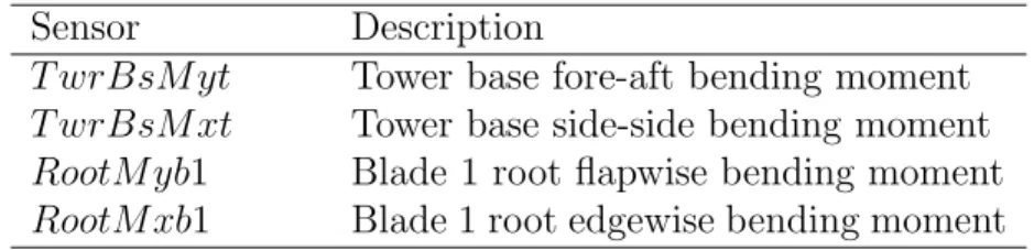
Out of the hundreds of sensorial output available from our simulations, we elect to retain only four for the sake of interpretability of the results and brevity of the publication, as shown in Table 4. These include the blade root and the tower base bending moments. Our presumption is to retain the sensorial output of aero-servo-elastic simulations that could, in the real-world, be directly deployed with little technical and economic cost if not already available in today’s structural health monitoring systems on WTs in the field using, for instance, fiber-based strain sensing.
Table 4: Retained sensorial output of aero-servo-elastic simulations.
Sensor Description
T wrBsM yt Tower base fore-aft bending moment T wrBsM xt Tower base side-side bending moment RootM yb1 Blade 1 root flapwise bending moment RootM xb1 Blade 1 root edgewise bending moment 3. Interpreting the simulations output
In this section we attempt to provide an interpretation of the numerical simulations, specifically with respect to the elementary effects of the inflow RVs on the short-term DEL of the blades and tower base in relation to the wake formation and transport. A qualitative analysis is here offered with the purpose of informing the subsequent GPR and sensitivity analysis.
3.1. Effect of mean wind speed U and turbulence σU
In Figure 5 the up-wind wind turbine is operating below rated power, which corresponds to a high thrust coefficient and high induction, thus leading into a significant wake deficit (lower wind speed in the wake) and an increase in turbulence. When the spacing is set to 3−5D the tower base fore-aft DEL of the wake-affected wind turbine is higher compared to DEL of the up-wind wind turbine. The high thrust coefficient and high induction from the up-wind wind turbine lead in reduction of the mean wind speed and an increase in the turbulence intensity of the transported wake towards the down-wind turbine. A wake-affected wind turbine experiences increased turbulence on the basis of two main contributions. Firstly, small-scale turbulence due the breakdown of tip vortices and turbulence generated by the shear layer in the edges of the wake and secondly from the meandering of the wake deficit relative to the position of the wake-affected rotor [24]. This increase in turbulence explains why the short-term tower base fore-aft DEL (welded steel) of the wake-affected wind turbine is higher compared to DEL of the up-wind wind turbine. This does not hold true for WTG separation between 8−11D, where turbulence and wind speed recovers, nor does it hold true for the blade root flap moment DEL. This implies a more pronounced effect of mean wind speed on the composite blades versus turbulence for the welded steel tower. For spacing above 8D the difference in DEL for both upwind and wake-affected wind turbine are marginal for both blades and tower structures. For wind speeds that lie above rated >11m/sand for a spacing of 3−5D, the upwind turbine tower base fore-aft DEL start to exceed that of the wake-affected wind turbine (figures omitted for brevity). This implies that the small scale mixing in the wake dominates the large scale effects of wake meandering, with the mean wind speed rendered the main driver of DEL. This may be attributed to less efficient transport of the wake meandering, as a result of lower thrust coefficient and induction on the rotor at higher wind speeds. It is further noted that for increasing mean wind speed, the gap in the blade root flapwise DEL reduces gradually between the upwind and wake affected wind turbine (figures omitted for brevity).
3.2. Effect of wind shear, α
Wind shear induces a periodic higher induction effect on one part of the rotor, which results in loss of symmetry for the wake deficit. This implies that elevated wind shear reduces the overall efficiency of the rotor, while creating a less severe wake in the process. This is particularly true for wind speeds above rated. This effect is well captured in Figure 6(c). The data is filtered to u ∈ [15−25]m/s above rated wind speed, where rotor induction is low to start with. The shear exponent is varied in ranges corresponding to α ∈ [0.05−0.11], α ∈ [0.13−0.18] and α ∈ [0.2−0.31]. When the shear exponent is low and in the narrow range α ∈ [0.05−0.11] the blade root flapwise bending moment DEL of the wake-affected wind turbine is shown to exceed the DEL of the up-wind wind turbine. When the shear exponent increases, the up-wind turbine exhibits higher DEL with respect to the wake-affected wind turbine. For wind speeds below rated, i.e., those corresponding to high thrust and high induction, as shown in Figure6(a), inefficiencies due to wind shear start to appear in the tail of the exceedence probabilities (corresponding toU ≈10m/s) for the blade root flapwise bending moment DEL of the wake-affected WT, with a reversal resulting in higher loads for α∈[0.05−0.11] compared to higher shear exponent ranges.
0.5 1 1.5 2 2.5 TwrBsMyt[kNm] 104 10-3
10-2 10-1 100
Pe
Up-wind Wake-affected
(a)Spacing 3−5D
0 2000 4000 6000 8000
RootMyb1[kNm]
10-4 10-3 10-2 10-1 100
Pe
Up-wind Wake-affected
(b)Spacing 3−5D
0.5 1 1.5 2 2.5
TwrBsMyt[kNm] 104 10-4
10-3 10-2 10-1 100
Pe
Up-wind Wake-affected
(c)Spacing 8−11D
0 2000 4000 6000 8000 10000 RootMyb1[kNm]
10-4 10-3 10-2 10-1 100
Pe
Up-wind Wake-affected
(d)Spacing 8−11D
Figure 5: Exceedence probabilities for tower base fore-aft bending moment DEL and blade root flapwise bending moment DEL conditional onu∈[3−10]m/s.
0 2000 4000 6000 8000
RootMyb1[kNm]
10-3 10-2 10-1 100
Pe
Up-wind, [0.05 0.11]
Wake-affected
Up-wind, [0.13 0.18]
Wake-affected
Up-wind, [0.2 0.31]
Wake-affected
(a)U∈[3−10]m/s
4000 5000 6000 7000 8000 9000 RootMyb1[kNm]
10-3 10-2 10-1 100
Pe
Up-wind, [0.05 0.11]
Wake-affected
Up-wind, [0.13 0.18]
Wake-affected
Up-wind, [0.2 0.31]
Wake-affected
(b)U∈[11−14]m/s
4000 6000 8000 10000
RootMyb1[kNm]
10-3 10-2 10-1 100
Pe
Up-wind, [0.05 0.11]
Wake-affected
Up-wind, [0.13 0.18]
Wake-affected
Up-wind, [0.2 0.31]
Wake-affected
(c)U∈[15−25]m/s
Figure 6: Exceedence probabilities for blade root flapwise bending moment DEL conditional on increasing shear exponent ranges, and spacing 3−5D.
3.3. Effect of horizontal inflow skewness, Ψ
In Figure 7a the up-wind wind turbine is operating below rated power, resulting in significant wake deficit, i.e., lower wind speed in the wake, and increase in turbulence. When the spacing amounts to 3−5D and the horizontal inflow skewness is negative Ψ∈[−10 −1], the tower base side-side bending moment DEL of the wake-affected WT is higher compared to DEL of the up-wind WT. However, this difference in Figure 7b vanishes once the horizontal inflow skewness becomes positive Ψ∈[1 10]. A similar effect of the horizontal inflow skewness is also observed on the blade root edgewise bending moment DEL as shown in Figure 7c and 7d.
1000 2000 3000 4000 5000 6000 TwrBsMxt[kNm]
10-3 10-2 10-1 100
Pe
Up-wind Wake-affected
(a)Ψ∈[−10 −1]
1000 2000 3000 4000 5000
TwrBsMxt[kNm]
10-2 10-1 100
Pe
Up-wind Wake-affected
(b)Ψ∈[1 10]
5500 6000 6500 7000
RootMxb1[kNm]
10-3 10-2 10-1 100
Pe
Up-wind Wake-affected
(c)Ψ∈[−10 −1]
5500 6000 6500 7000 7500
RootMxb1[kNm]
10-3 10-2 10-1 100
Pe
Up-wind Wake-affected
(d)Ψ∈[1 10]
Figure 7: Exceedence probabilities for tower base side-side bending moment DEL and blade root edgewise bending moment DEL, conditional onu∈[3−10]m/s, and spacing 3−5D.
3.4. Recommendations
This work aims to establish a data-driven model to predict the loads in the wake-affected WT, relying on loads measurements extracted from adjacent WTs, operating on availability of sparse structural measurements across the farm. From a structural health monitoring and life cycle as- sessment point of view, the following guidelines/recommendations can be suggested for inflow RVs:
• We recommend acquiring wind inflow turbulence data with high accuracy and precision, primarily for wind speeds below rated, when the aim lies in yielding a confident predic- tor/surrogate of the tower base fore-aft DEL loads of the wake-affected wind turbine.
• We recommend acquiring wind inflow shear data with high accuracy and precision, primarily for wind speeds corresponding to maximum thrust (i.e. U ≈ 10m/s) and above rated wind speed (i.e. U ∼> 14m/s), when the aim lies in yielding a confident predictor/surrogate of blade flap DEL loads of the wake-affected wind turbine.
• We recommend acquiring horizontal inflow skewness data with high accuracy and precision, primarily for wind speeds below maximum thrust (i.e. U ∼< 10m/s), when the aim lies in yielding a confident predictor/surrogate of the tower base side-side and blade root edgewise DEL loads of the wake-affected wind turbine.
4. Methodological framework
4.1. Gaussian Processes
Consider the function f(xxx) ∈ R of the input vector xxx ∈ Rn. The function f(·) is referred to as a Gaussian Process (GP) if its value, when sampled on a finite number of inputs XXX = xxx1 xxx2 · · · xxxN
, follows the multivariate normal distribution N (µµµ(XXX), KKK(XXX, XXX)), with mean µµµ(XXX) = E{fff(XXX)}and covarianceKKK(XXX, XXX) = E
(fff(XXX)−µµµ(XXX))·(fff(XXX)−µµµ(XXX))> , wherefff(XXX) = f(xxx1) f(xxx2) · · · f(xxxN)T
[36, Sec. 2.2]. In turn, the mean and covariance are of the form:
µµµ(XXX) =
µ(xxx1) µ(xxx2)
... µ(xxxN)
KKK(XXX, XXX) =
k(xxx1, xxx1) k(xxx1, xxx2) · · · k(xxx1, xxxN) k(xxx2, xxx1) k(xxx2, xxx2) · · · k(xxx2, xxxN)
... ... . .. ... k(xxxN, xxx1) k(xxxN, xxx2) · · · k(xxxN, xxxN)
(8)
where k(xxxi, xxxj) is the respective covariance function, a symmetric positive definite function which measures the similarity between the pair of input RVsxxxi andxxxj. The GP is determined by the mean and covariance functions. Hereafter, the mean function is assumed as zero, while the covariance kernel is selected as the squared exponential, which is defined as follows [36, pp. 83-84]:
k(xxx, xxx0) = σ2f ·exp −1 2
n
X
i=1
`2i ·(xi−x0i)2
!
(9) where σ2f :=k(xxx, xxx) is the function variance, and`2i, i= 1, . . . , n are scaling factors for each one of the input dimensions. The scaling factors determine the smoothness of the function on the respective input dimension: a very large value indicates large differences between adjacent points, thus leading to non-smooth behavior; a very small value indicates significant similarity between remote points, and suggests that there are no significant variations on the signal. As will be explained later, these values are adjusted to the observed data, while the obtained scaling factors can be used to determine the influence of the input dimensions on the function outcomes.
4.2. Gaussian Process regression
In a Gaussian Process Regression (GPR), the covariance kernel is utilized to associate the function values observed on a set of training points,XXX =
x
xx1 xxx2 · · · xxxN
, to a test input vector xxx∗, and thus provide an estimate of the function value on the test point. To this end, it is first assumed that a set of noisy values of the function are observedyi,i= 1, . . . , N, whereyi =f(xxxi)+wi with wi a zero-mean normally and independently distributed process, with variance σ2w. The noisy function values, grouped in the vector yyy :=
y1 y2 · · · yNT
, and the function value on the test input f(xxx∗) are jointly normally distributed variables, as follows [36, Sec. 2.2]:
f(xxx∗) y yy
∼ N
0 000N×1
,
k(xxx∗, xxx∗) kkk(xxx∗, XXX) k
kk(XXX, xxx∗) KKK(XXX, XXX) +σ2wIIIN
(10) wherekkk(xxx∗, XXX) =kkkT(XXX, xxx∗) =
k(xxx∗, xxx1) · · · k(xxx∗, xxxN)
is the cross-covariance between the test and the training input vectors. Then, using the properties of the multivariate normal distribution, the distribution of the function on the test input conditioned on the the training noisy function valuesyyy is also Gaussian, as follows [36, Sec. 2.2]:
p(f(xxx∗)|yyy, XXX) =N f¯(xxx∗), Q(xxx∗)
(11) with conditional mean ¯f(xxx∗) and variance Q(xxx∗), which are calculated as follows:
f(x¯xx∗) =kkk∗· KKK+σw2IIIN
−1
yyy (12a)
Q(xxx∗) = k∗−kkk∗· KKK+σ2wIIIN−1
·kkkT∗ (12b)
and where k∗ :=k(xxx∗, xxx∗),kkk∗ :=kkk(xxx∗, XXX), andKKK :=KKK(XXX, XXX).
4.3. Bayesian approach for adjustment of the hyperparameters of the GPR
The performance of the GPR is defined by the kernel parameters, comprised by σf2, `2i for i= 1, . . . , n, and σ2w, which are jointly referred to as the hyperparametersP :={σw2, σf2, `21,· · ·, `2n}.
Often, the GPR hyperparameters are optimized via maximization of themarginal likelihood, defined as follows [36, Sec. 2.3]:
lnp(yyy|XXX,P) =−1
2yyyT KKK+σ2wIIIN−1
y y y−1
2
KKK+σ2wIIIN − N
2 ln 2π (13)
This is a non-linear optimization problem, which is typically solved by gradient-based non-linear optimization methods with the help of the partial derivatives of the marginal likelihood with re- spect to each one of the hyperparameters. This optimization results in point estimates of the hyperparameters.
Contrariwise, Bayesian methods aim at determining a distribution for the hyperparameters given the available data, based on some original assumptions on the hyperparameter distribution.
Therefore, Bayesian methods aim at calculating the hyperparameter posterior distribution [38, pp. 12-13]:
p(P|yyy, XXX) = p(yyy|XXX,P)·p(P)·p−1(yyy|XXX) (14) where p(P) is the prior hyperparameter distribution, which encapsulates any a-priori knowledge of the hyperparameter distribution, and p(yyy|XXX) comprises the model evidence, defined as follows:
p(yyy|XXX) :=
Z
Ω
p(yyy|XXX,P)·p(P) dP (15) where Ω represents the space where P is defined.
In the case of GPR, an analytical expression for the hyperparameter posterior is not possible, due to the non-linear interaction of the hyperparameters with the likelihood. Instead, Markov Chain Monte Carlo (MCMC) methods can be used to obtain a sample of the hyperparameter posterior [38, Ch. 6-7]. In the analysis presented below, the Metropolis-Hastings algorithm is used for this purpose. Further details on the Metropolis-Hastings sampling method can be found [38, Ch. 7].
4.4. Sensitivity analysis based on the GPR input scaling factors
The input scaling factors `2i associated with the squared exponential kernel function defined in Eq. (9) determine the smoothness of the kernel on the respective input dimensionxi. Large positive values of`2i indicate a very rough behavior of the function on the dimensionxi [36, pp. 21-22]. This happens because the correlation between values on xi and xi+ ∆x, with ∆x a small increment, drops very fast. Otherwise, values of`2i close to zero indicate that the function is essentially flat on the dimension xi [36, pp. 21-22]. In this case, the increment ∆x required to produce a significant change in the correlation needs to be very large. This property can be used as a way to evaluate the sensitivity of a function approximated by a GPR to each one of the input dimensions. This is shown below.
The squared exponential kernel in Eq. (9) can be factorized as follows:
k(xxx, xxx0) =σf2 ·
n
Y
i=1
exp
−1
2`2i ·(xi−x0i)2
=σ2f ·
n
Y
i=1
ki(xi, x0i) (16) ki(xi, x0i) := exp
−1
2`2i ·(xi−x0i)2
and thus the contribution of input xi to the kernel can be decoupled. The value ∆xρis here defined as the increment in xi required to decrease by a value ρ the maximum covariance value. More precisely ∆xρ ∈R+ is the value such that:
ki(xi, xi+ ∆xρ) =ki(xi, xi)−ρ (17) with 0 < ρ 1 a small positive number. Applying the definition of ki(xi, x0i) and using the fact that ki(xi, xi) = 1, then:
exp
−1
2`2i ·∆x2ρ
= 1−ρ (18)
and then, solving for ∆xρ, the following value is obtained:
∆xρ =`−1i ·p
−2·ln(1−ρ) (19)
The value ∆xρ can be interpreted as the distance required to move along the i-th input to decrease the correlation (similarity) between the function valuesf(xi) andf(xi+ ∆xρ) by the value ρ. If the value of ∆xρis larger than the range of the data on the i-th input, then the desired change in the correlation is not feasible. With ρ close to zero, this resut would be an indicator of flatness of the function in the direction xi. In turn, this indicates that the function f(xxx) is insensitive to the input xi.
Note that although ∆xρ can just be interpreted as the inverse of`i, and both variables hold the same information, ∆xρ facilitates understanding of the GPR sensitivity towards a certain input.
4.5. Kullback-Leibler divergence for comparison of GPRs
Consider two GPRs represented as Ma :={yyya, XXXa,Pa} and Mb :={yyyb, XXXb,Pb}, with different training data and hyperparameters. Then, it is necessary to evaluate whether or not the prediction of GPRsMaandMb at a test pointxxx∗is the same. Considering that the GPR prediction at the test point follows a Gaussian distribution, it is possible to use the Kullback-Leibler (KL) divergence to compare if both predictive distributions are the same [9, p. 57]. The KL divergence for a Gaussian distribution takes the form:
DKL(xxx∗|Ma,Mb) = 1 2
Qa(xxx∗)
Qb(xxx∗) + ( ¯fa(xxx∗)−f¯b(xxx∗))2
Qb(xxx∗) + lnQb(xxx∗) Qa(xxx∗) −1
(20) where ¯fj(xxx∗) and Qj(xxx∗), with j = {a, b}, are the GPR predictive mean and variance calculated with Eq. (12) for each corresponding model.
The global KL divergence of the predictions obtained with both GPRs can be obtained by integrating over the whole domain X ⊆ Rn, as follows:
DKL(Ma,Mb) = Z
X
DKL(xxx|Ma,Mb) dxxx (21) while a marginalized KL divergence for input xi, i= 1, . . . , n can be obtained by integrating with respect to the remaining inputs, as follows:
DKL(xi|Ma,Mb) = Z
X∼i
DKL(xxx|Ma,Mb) dxxx∼i (22) where xxx∼i represents the input vector after eliminating input xi, and X∼i is its respective space.
Evaluation of the integrals in Eqns. (21) and (22) is not analytically tractable, and instead, numerical approximations are required. The construction of the global and marginalized KL divergences in Eqns. (21) and (22) is based on the assumption that there are no cross-correlations in the predictive distribution, or more precisely,
E
(f(xxx∗1)−f¯(xxx∗1))·(f(xxx∗2)−f¯(xxx∗2))|yyy, XXX = 0 (23) forxxx∗1 6=xxx∗2. Although this assumption does not comply with the definition of the GP, it largely simplifies the calculation of the global and marginalized KL divergences.
5. Results
5.1. Prediction and analysis of DELs from local EOPs
In this initial analysis, GPR models are built to predict the DELs of a single WT component based on locally measured EOPs. This corresponds to the ideal case when all the WTs are fully instrumented and a complete set of wind field parameters are available on each wind turbine. The objective of this initial analysis is to determine which input variables mostly affect the DELs and to determine if there are significant differences between the loads in the up-wind and wake-affected WTs at different structural components.
Accordingly, in the present case the input vector xxx∈R4 is made up by the 10 minute averages of the wind speed U := x1, turbulence intensity σ := x2, shear exponent α := x3, and inflow horizontal skewness Ψ := x4 of the respective WT. In turn, the outputy corresponds to the DELs calculated from the respective 10 minute loads measured either in the root of one of the blades in the edgewise or flapwise directions, or in the tower base in the fore-aft or side-to-side directions. For the construction of the regression, the range of the input variables is normalized within the interval [0,1], while the values of the DELs are scaled down by a factor of 104. This normalization is used to enhance the numerical stability of the models. Individual GPRs are built for the DELs obtained on the up-wind and wake-affected WTs at different spacing configurations and with different W¨ohler exponents.
5.1.1. Hyperparameter identification
The Bayesian inference approach based on the Metropolis-Hastings (MH) sampling algorithm described in Section 4.3, is used to estimate of the posterior hyperparameter distribution of the GPR predictor based on the available coupled DWM-FAST simulations. To this end, 180 input- output pairs are randomly selected to calculate the GPR’s marginal likelihood (Eq. (13)) within the MH sampling loop, while the remaining ones are used for posterior model validation. To ensure even distribution of the training samples, a sampling approach based on clustering of the complete set of inputs is performed. More precisely, an agglomerative hierarchical clustering tree based on Ward’s linkage on the Euclidean distance is applied. Subsequently, 180 clusters are built based on
the obtained linkage and a single input and its respective output are randomly extracted from each one of them.
Independent log-normal distributions are defined for each one of the hyperparameters. Similarly, independent log-normal distributions are selected as proposal distributions. The parameters of these distributions are summarized in Table 5.
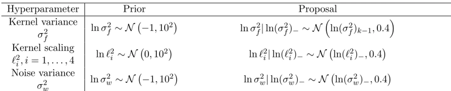
Table 5: Settings of the Metropolis-Hastings algorithm for sampling of the GPR hyperparameter posterior
Hyperparameter Prior Proposal
Kernel variance
lnσ2f ∼ N −1,102
lnσf2|ln(σ2f)− ∼ N
ln(σ2f)k−1,0.4 σf2
Kernel scaling
ln`2i ∼ N 0,102
ln`2i|ln(`2i)−∼ N ln(`2i)−,0.4
`2i, i= 1, . . . ,4 Noise variance
lnσ2w∼ N −1,102
lnσw2|ln(σ2w)−∼ N ln(σw2)−,0.4 σw2
Number of Monte-Carlo samples 104. The symbols (σf2)−, (`2i)−, and (σw2)− indicate the values of the same quantity drawn in the previous iteration of the MH sampling algorithm.
Using the previously described set-up, a total of 10 000 samples are simulated with the MH algorithm. Figure 8 displays the distribution of the GPR hyperparameters based on the sample of the hyperparameter posterior drawn with the MH algorithm, obtained with the data from the up-wind WT tower edgewise and flapwise DELs. It is first noted that although the initial values and prior distributions are similar for all the GPR hyperparameters, the posterior distributions converge to different intervals. The distributions for the noise variance, kernel variance and the first three scale parameters (`21 : wind speed;`22 : turbulence intensity; `23: shear exponent) are quite narrow,`24 : horizontal inflow skewness, has wider distributions in both edgewise and flapwise DELs.
The latter seems to indicate that the horizontal inflow skewness has a reduced effect in the DELs.
Further analysis based on the obtained GRPs is provided in the sequel.
Figure 8: Boxplots displaying the distribution of the GPR hyperparameters sampled with the MH algorithm for the DELs in the blade edgewise and flapwise directions. W¨ohler exponent: 9.
5.1.2. Analysis of DELs based on the obtained GPRs
Response surfaces. After estimation of the hyperparameter posterior, it is possible to calculate response surfaces of the DEL for any values in the input space. For instance, 1D slices displaying the DEL as a function of single input variables while the remaining ones are kept fixed can be calculated with the help of the obtained GPR. Figs. 9and10display slices of the DEL in the blade –edgewise and flapwise direction– extracted from the GPR with Maximum A Posteriori (MAP) hyperparameter estimates on the up-wind and down-wind WTs. On each frame, the remaining inputs are set to the sample median values, while the spacing between WTs is 11 rotor diameters, and the W¨ohler exponent is m = 9. In both cases, the GPR predictive mean is similar in both the up-wind and wake-affected WTs, while a significant decrement is found in the DEL of the wake- affected WT at high wind speeds. On the other hand, the confidence intervals are well confined around the mid-part of the input range, while the dispersion increases towards the boundaries of the input ranges. The increased dispersion is observed due to the reduced number of points towards the boundaries.
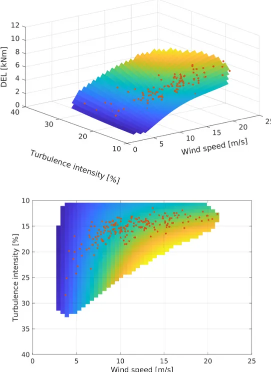
Figure 11 shows the GPR predictive mean of the DEL in the blade flapwise direction as a function of wind speed and turbulence intensity (α and Ψ set to their median values, d = 11, and m = 9). DEL estimates with variance higher than 50 times the minimum predictive variance are censored in the displayed surfaces. As observed in Figure 10, the DEL in the blade flapwise direction increases as the wind speed and the turbulence intensity do, with the wind speed making
Figure 9: Slices of the DEL predictive mean and 99% confidence intervals (CI) based on a GPR with MAP hyperparameter estimates obtained on the blade in the edgewise direction in the up-wind and down-wind WTs.
Other inputs are kept at their training set sample median values indicated on each frame. WT spacing: 11 diameters;
W¨ohler exponent: 9.
Figure 10: Slices of the DEL predictive mean and 99% confidence intervals (CI) based on a GPR with MAP hyperparameter estimates obtained on the blade in the flapwise direction in the up-wind and down-wind WTs.
Other inputs are kept at their training set sample median values indicated on each frame. WT spacing: 11 diameters;
W¨ohler exponent: 9.
the maximum effect. The training data points, displayed as red dots in the surface, coincide with the GPR predictive mean, but also are confined to the non-censored area, which indicates that the predictive variance is well-bounded around the area spanned by the training points. In practice, DEL estimates in points outside the non-censored area can be deemed as unreliable, while at the same time have a low probability of occurrence, according to the joint distribution of U and σ.
Error analysis. The predictive performance of the GPR is measured in terms of the Normalized Mean Squared Error (NMSE) calculated on the validation set. The NMSE is defined as:
NMSE =
PNval
i=1 (yi−f(x¯xxi))2 PNval
i=1 yi2 (24)


![Figure 5: Exceedence probabilities for tower base fore-aft bending moment DEL and blade root flapwise bending moment DEL conditional on u ∈ [3 − 10] m/s.](https://thumb-eu.123doks.com/thumbv2/1library_info/5304318.1678196/11.918.101.835.101.681/figure-exceedence-probabilities-bending-moment-flapwise-bending-conditional.webp)
![Figure 7: Exceedence probabilities for tower base side-side bending moment DEL and blade root edgewise bending moment DEL, conditional on u ∈ [3 − 10] m/s, and spacing 3 − 5D.](https://thumb-eu.123doks.com/thumbv2/1library_info/5304318.1678196/12.918.98.835.299.893/figure-exceedence-probabilities-bending-edgewise-bending-conditional-spacing.webp)