Exercise 9: Synthesis of MIMO Control Systems
We have learned that MIMO systems are more complicated than SISO systems and therefore their control as well. In fact, it is very difficult to apply intuitive concepts like loop shaping, that apply to SISO systems, because of the cross couplings/interactions between the inputs and the outputs. This means that systematic methods should be used, in order to achieve good control properties. We define two big groups of methods, that are used nowadays:
• H2 methods: Optimization problems in time domain which try to minimize the error signal over all frequencies.
• H∞ methods: Optimization problems in frequency domain which try to minimize the error signal over all frequencies.
9.1 The Linear Quadratic Regulator (LQR)
We first look at one H2 method: the linear quadratic regulator.
9.1.1 Definition
With the given state-space description d
dtx(t) =A·x(t) +B·u(t), A∈Rn×n, B ∈Rn×m, x(t)∈Rn, u(t)∈Rm (9.1) we are looking for a state-feedback controller
u(t) = f(x(t), t), (9.2)
that brings x(t) asymptotically to zero (with x(0) 6= 0). In other words it should hold.
t→∞lim x(t) = 0. (9.3)
Remark. The input u(t) we want to control depends only on x(t) and not on other dynamic state variables.
In order to achieve the best control, we want to minimize the criterium J(x, u) =
Z ∞ 0
(x|·Q·x
| {z }
error
+u|·R·u
| {z }
given energy
) dt, (9.4)
where
Q∈Rn×n (9.5)
is a symmetric positive semidefinite matrix and
R ∈Rm×m (9.6)
is a symmetric positive definite matrix. These two matrices represent the weights, i.e. the importance, of two things: how fast does the controller bringx(t) to zero and how much energy should it use.
Remark. In the SISO case, we deal with scalars and things arenicer: J(x, u) =
Z ∞
(q·x2+r·u2)dt, (9.7)
Example 1. Let’s try to visualize this: a criterion could look like J(x, u) =
Z ∞ 0
x21+ 6·x1·x2+ 100·x22+ 6·u21+ 10·u22 dt.
The matricesQ and R are
Q=
1 3 3 100
and
R =
6 0 0 10
The solution1 u(t) = f(x(t), t) (that minimizes (9.4) ) is given as
u(t) =−K·x(t), (9.8)
with
K =R−1·B|·Φ. (9.9)
where Φ is the solution of the Riccati equation
Φ·B ·R−1·B|·Φ−Φ·A−A|·Φ−Q= 0. (9.10) Remark. The actual procedure to determine this equation is not trivial. The main point you should be concerned with in this course is the following: we are trying to minimize the given criterium and we are dealing with matrices. This means that in the end, we calculate matrix derivations and minimize, obtaining matrix equations. If you are interested in the minimization procedure have a look here.
Remark. Don’t forget what we are trying to do! This equations give us the optimal controller K: this means but not that it will be always the best one.
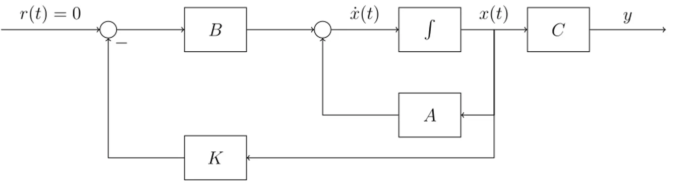
The feedback loop of such a system can be seen in Figure 1.
B R
C
A K
r(t) = 0 x(t)˙ x(t) y
−
Figure 1: LQR Problem: Closed loop system.
1Here, it is assumed that x(t) is already available. This is normally not the case and we will therefore introduce an element (observer) that gives us an estimation of it (see next chapters).
9.1.2 Kochrezept
(I) Choose the matrices Qand R:
• The matrix Qis usually chosen as follows:
Q= ¯CT ·C,¯ C¯ ∈Rp×n (9.11) where
p= rank(Q)≤n. (9.12)
Equation 9.11 represents the full-rank decomposition of Q. This makes sure that the therm with Q in the criterion contains enough informations about the state’s behaviour. ¯C has strictly speaking nothing to do with the state space description’s matrix C. We will however discover, that the choice ¯C =C is really interesting.
• The matrix R is usually chosen as follows:
R=r·1m×m. (9.13)
(II) Find the symmetric, positive definite solution Φ of the Riccati equation
Φ·B ·R−1·B|·Φ−Φ·A−A|·Φ−Q= 0. (9.14) Remark. Such a solution exists if
• The pair {A, B} is completely controllable and
• The pair {A,C}¯ is completely observable.
This doesn’t mean that these conditions should be always fulfilled: sufficient, not nec- essary.
(III) Compute the matrix of the controllerK with
K =R−1·B|·Φ. (9.15)
9.1.3 Frequency Domain
By looking at Figure 1 one can write
LLQR(s) = C·(s·1−A)−1·B (9.16) and
TLQR(s) =C·(s·1−(A−B ·K))−1 ·B. (9.17) 9.1.4 Properties
A bunch of nice properties can be listed:
• The matrix of the closed-loop system
A−B·K (9.18)
is guaranteed to be a Hurwitz matrix.
Remark. A Hurwitz matrix is a matrix that has all eigenvalues withnegative real parts.
But wait, what does it mean? We have learned that eigenvalues with negative real parts contribute to the stability of the closed-loop system. In this case is the closed-loop system asymptotically stable.
• If one choosesR =r·1one gets for the minimal return difference
• IfQ >> R we say that we have cheap control energy.
• IfR >> Q we say that we have expensive control energy.
µLQR= min
ω {σmin(1+LLQR)} ≥1. (9.19)
• Closed-loop behaviour:
maxω {σmax(S(j·ω))} ≤1, (9.20) maxω {σmax(T(j·ω))} ≤2. (9.21)
• Of course you are not expected in real life to solve the Riccati equation by hand. Since these calculations contain many matrix multiplications, numerical algorithms are devel- oped. Matlab offers the command
K=lqr(A,B,Q,R);
• Remind that
Φ = ΦT (9.22)
9.1.5 Pole Placement
Another intuitive way of approaching this problem is the so called pole placement. Given that one knows that the state feedback matrix is A−B·K, one can choose such a K matrix, that the desired poles are achieved. With this method one can have direct influence on the speed of the control system. The disadvantage, however, is that one has no guarantee of robustness.
If one looks at Figure 2, one can derive the following complete state space description of the plant and of the controller:
˙
x(t) = A·x(t) +B ·u(t), y(t) = C·x(t) +D·u(t),
˙
z(t) = F ·z(t) +G·e(t), u(t) = H·z(t),
(9.23)
where e(t) is the error of the controller.
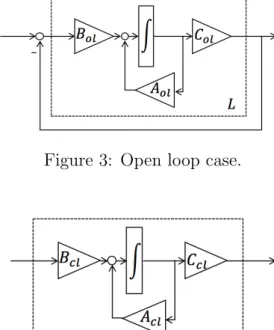
Open Loop Conditions
By assuming for this case D = 0 and plugging the information of the controller in the plant, one gets
˙
x(t) = A·x(t) +B·Hz(t), y(t) = C·x(t),
˙
z(t) = F ·z(t) +G·e(t).
(9.24)
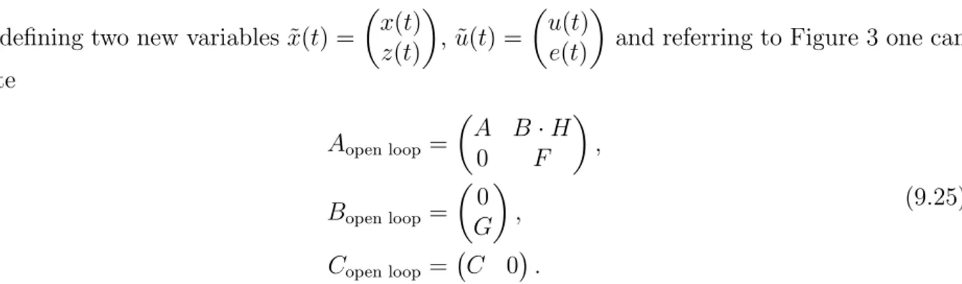
By defining two new variables ˜x(t) = x(t)
z(t)
, ˜u(t) = u(t)
e(t)
and referring to Figure 3 one can write
Aopen loop =
A B·H
0 F
, Bopen loop =
0 G
, Copen loop = C 0
.
(9.25)
Remark. Because of the rule for determinant of matrices build up from other submatrices, we automatically know that the eigenvalues ofAopen loopare the eigenvalues ofAand the eigenvalues of F. Mathematically
λ(Aopen loop) = λ(A) +λ(F). (9.26)
Closed Loop Conditions
It is still assumed D= 0. If one closes the loop it holds
e(t) =−y(t)⇒ e(t) = −C·x(t). (9.27) This gives the state space description
˙
x(t) = A·x(t) +B ·Hz(t), y(t) = C·x(t),
˙
z(t) = F ·z(t) +G·(−C·x(t)).
(9.28)
By defining a new variable ˜x(t) = x(t)
z(t)
and referring to Figure 4 one can write
Aclosed loop =
A B·H
−G·C F
. (9.29)
Remark. The eigenvalues of Aclosed loop are not well defined. Moreover it holds
λ(Aclosed loop) =f(F, G, H). (9.30)
This makes this method extremely superficial and not generally useful.
Figure 2: Signal Flow Diagram with Controller.
Figure 3: Open loop case.
Figure 4: Closed loop case.
9.1.6 Examples
Example 2. Your task is to keep a space shuttle in its trajectory . The deviations from the desired trajectory are well described by
d
dtx(t) = A·x(t) +b·u(t)
= 0 1
0 0
·x(t) + 0
1
·u(t).
x1(t) is the position of the space shuttle and x2(t) is its velocity. Moreover, u(t) represents the propulsion. The position and the velocity are known for every moment and for this reason we can use a state-feedback regulator. In your first try, you want to implement a LQR with
Q=
1 0 0 2.25
R = 4.
(a) Show that the system is completely controllable.
(b) Find the state feedback matrix K.
After some simulations, you decide that the controller you’ve found is not enough for your task.
Your boss doesn’t want you to change the matrices Q and R and for this reason you decide to try with direct pole placement. The specifications are
• The system should not overshoot.
• The error of the regulator should decrease withe−3·t. (c) Find the poles such that the specifications are met.
(d) Find the new state feedback matrix K2.
Solution.
(a) The controllybility of the system is easy to show: the controllability matrix is R2 = b A·b
= 0 1
1 0
. The rank of R is clearly 2: completely controllable.
(b) In order to find the matrix K, one has to compute the solution of the Riccati equation related to this problem. First, one has to look at the form that this solution should have.
Hereb is a 2×1 vector. This means that since Φ = ΦT we are dealing with a 2×2 Φ of the form
Φ =
ϕ1 ϕ2 ϕ2 ϕ3
With the Riccati equation, it holds
Φ·B·R−1·B|·Φ−Φ·A−A|·Φ−Q= 0 Plugging in the matrices one gets
Φ· 0
1
·4−1· 0
1 T
·Φ−Φ· 0 1
0 0
− 0 1
0 0 T
·Φ−
1 0 0 2.25
= 0 0
0 0 1
4 · ϕ2
ϕ3
· 0 1
·
ϕ1 ϕ2 ϕ2 ϕ3
−
0 ϕ1 0 ϕ2
−
0 0 ϕ1 ϕ2
−
1 0 0 2.25
= 0 0
0 0 1
4 ·
0 ϕ2
0 ϕ3
·
ϕ1 ϕ2
ϕ2 ϕ3
−
1 ϕ1
ϕ1 2·ϕ2+ 2.25
= 0 0
0 0 1
4 ·
ϕ22 ϕ2·ϕ3 ϕ2·ϕ3 ϕ23
−
1 ϕ1 ϕ1 2·ϕ2+ 2.25
= 0 0
0 0
ϕ22
4 −1 ϕ24·ϕ3 −ϕ1
ϕ2·ϕ3
4 −ϕ1 ϕ423 −2·ϕ2−2.25
= 0 0
0 0
.
From this it follows:
• ϕ422 −1⇒ ϕ2 =±2.
• From the fourth term, we get two cases:
– ϕ2 = 2: ϕ3 =√
25 =±5.
– ϕ2 =−2: ϕ3 =j ·√ 7.
• Because of theSylvester’s Criterion,ϕ1 should be positive, in order to get a positive definite matrix. Plugging into the second term: ϕ1 = ϕ24·ϕ3 = 2.5 is the only positive solution. This means that the only reasonable choice isϕ2 = 2 andϕ3 = 5.
We therefore get
Φ =
2.5 2
2 5
Because of the Sylvester’s Criterion and the fact that Φ should be positive definite, this is a good matrix!
For the matrix K it holds
K =R−1·B|·Φ
= 1
4 · 0 1
·
2.5 2 2 5
= 1
4 · 2 5 .
(c) Overshoot or in general oscillations, are due to the complex part of some poles. The real part of these poles is given by the decrease function of the error:
π1 =π2 =−3 (d) The closed loop has feedback matrix
A−B ·K2
We have to choose K2 such that the eigenvalues of the state feedback matrix are both
−3. The dimensions ofK2 are the same as the dimensions of K, namely 1×2. It holds A−B·K2 =
0 1 0 0
− 0
1
· k1 k2
= 0 1
0 0
−
0 0 k1 k2
=
0 1
−k1 −k2
. The eigenvalues of this matrix are
π1,2 = −k2±p
k22−4k1 2
Since the two eigenvalues should have the same value, we know the the part under the square rooth should vanish. This means that −k22 =−3⇒k2 = 6. Moreover:
k1 = k22 4
= 9.
The matrix finally reads
K2 = 9 6 .
Example 3. A system is given as
˙
x1 = 3·x2
˙
x2 = 3·x1−2·x2+ 1 2·u y= 4·x1+ 7
3·x2. (a) Solve the LQR problem for the criterion
J = Z ∞
0
7·x21+ 3·x22+1 4 ·u2dt and find K.
(b) Find the eigenvalues of the closed-loop and the LQ regulatorK.
(c) Does it change something if we use the new criterion?
Jnew = Z ∞
0
70·x21+ 30·x22+ 10 4 ·u2dt
Solution.
(a) From the theory of the course Lineare Algebra I/II about the quadratic forms, one can read
Q= 7 0
0 3 and
R = 1 4.
The state-space description of the system can be rewritten as x˙1
˙ x2
=
0 3 3 −2
| {z }
A
· x1
x2
+ 0
1 2
| {z }
B
·u
y= 4 73
| {z }
C
· x1
x2
+ 0
|{z}
D
·u.
Plugging this into the Riccati equation one gets:
Φ· 0
1 2
·4· 0 12
·Φ−Φ·
0 3 3 −2
−
0 3 3 −2
·Φ− 7 0
0 3
= 0 0
0 0 2ϕ2
2ϕ3
· ϕ22 ϕ23
−
3ϕ2 3ϕ1−2ϕ2 3ϕ3 3ϕ2−2ϕ3
−
3ϕ2 3ϕ3 3ϕ1−2ϕ2 3ϕ2−2ϕ3
− 7 0
0 3
= 0 0
0 0 ϕ22 ϕ2ϕ3
ϕ2ϕ3 ϕ23
−
6ϕ2+ 7 3ϕ1−2ϕ2+ 3ϕ3 3ϕ1−2ϕ2+ 3ϕ3 6ϕ2−4ϕ3+ 3
= 0 0
0 0
Hence, one gets 3 equations (two elements are equal because of symmetry):
ϕ22 −6·ϕ2−7 = 0 ϕ2·ϕ3−3·ϕ1+ 2·ϕ2−3·ϕ3 = 0 ϕ23−6·ϕ2+ 4·ϕ3−3 = 0 From here, with the same procedure we have used before, one gets
Φ = 34
3 7
7 5
. This gives K as
K = 4· 0 12
· 34
3 7
7 5
= 14 10 . (b) The matrix to analyze is
A−B·K =
0 3 3 −2
− 0
1 2
· 14 10
=
0 3 3 −2
− 0 0
7 5
=
0 0
−4 −7
.
The eigenvalues of the closed loop system are given with det((A−B·K)−λ·1) = 0
λ2+ 7λ+ 12 = 0 from which it follows: λ1 =−3 andλ2 =−4.
(c) No. K remains the same, because it holds Jnew = 10·J.
Example 4. You have to design a LQ regulator for a plant with 2 inputs, 3 outputs and 6 state variables.
(a) What are the dimensions of A, B, C and D?
(b) What is the dimension of the transfer function u→y?
(c) What is the dimension of the matrixQ of JLQR? (d) What is the dimension of the matrixR of JLQR?
(e) What is the dimension of the matrixK?
Solution.
(a) One can find the solution by analyzing the meaning of the matrices:
• Since we are given 6 states variables, the matrixAshould have 6 rows and 6 columns, i.e. A∈R6×6.
• Since we are given 2 inputs, the matrix B should have 2 columns and 6 rows, i.e.
B ∈R6×2.
• Since we are given 3 outputs, the matrix C should have 6 columns and 3 rows, i.e.
C∈R3×6.
• Since we are given 2 inputs and 3 outputs, the matrixD should have 2 columns and 3 rows, i.e. D∈R3×2.
(b) Since we are dealing with a system with 2 inputs and 3 outputs,P(s)∈R3×2. Moreover, P(s) should have the same dimensions of D because of its formula.
(c) From the formulation of Q one can easily see that its dimensions are the same of the dimensions of A, i.e. Q∈R6×6.
(d) From
u(t) = −K·x(t)
we can see thatK should have 6 columns and 2 rows, i.e. K ∈R2×6.