Lecture 9: Linear Quadratic Regulator

Lecture 9: Linear Quadratic Regulator

1 LQR

Motivation:

Last week, we introduced the concept o state feedback, with the idea of using the states of the system and its dynamics to synthesize a controller using desired pole-placement.

This week we introduce Linear Quadratic control (LQ) and the special case of the Linear Quadratic Regulator (LQR). The concept behind this control strategy has a key role for control theory and is worth a detailed explanation.

Moreover, pole placement has some drawbacks:

• Does not work well with model uncertainty.

• Does not allow specific tuning of desired trade-offs (e.g. cost vs. performance).

1.1 Problem Definition

Given the dynamics of a system d

dtx(t) =A·x(t) +B·u(t), A∈R^n×n, B ∈R^n×m, x(t)∈Rⁿ, u(t)∈R^m (1.1) find a controller

u(t) =f(x(t), t), t∈[0,∞] (1.2) that brings x(t) asymptotically to zero (with x(0) 6= 0). In other words it should hold:

t→∞lim x(t) = 0, (1.3)

i.e. the cost

J_LQR(x(t), u(t)) = Z ∞

0

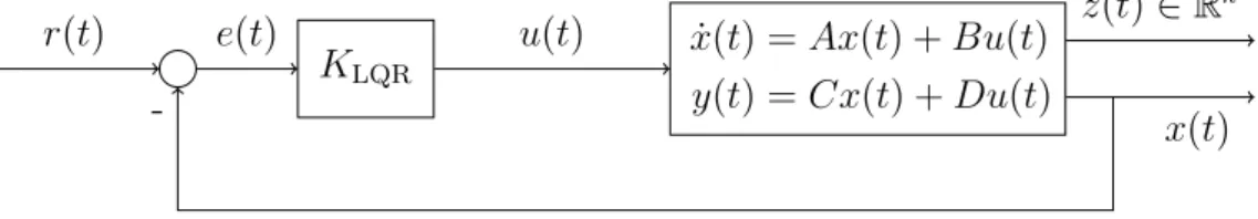
kz(t)k²₂+ρku(t)k²₂dt, ρ∈R⁺ (1.4) is minimized, where ρ allows trade-off between energy of the input and energy of the controlled signal and z(t) = Ex(t) +F u(t) can be chosen to contain the state variables of interest. The LQR standard control loop is reported in Figure 1.

K_LQR x(t) =˙ Ax(t) +Bu(t) y(t) = Cx(t) +Du(t)

r(t) e(t) u(t) z(t)∈R^k

- x(t)

Figure 1: LQR Problem: Closed loop system.

1.2 General Form

1.2.1 Preliminary Definitions

Since the cost function introduced in Equation 1.4 contains the euclidean norm, one recalls its definition:

ku(t)k²₂ =u(t)^|u(t)

=X

i

u_i(t)². (1.5)

The weighted euclidean norm reads

ku(t)k²_R,2 =u(t)^|Ru(t). (1.6) Definition 1. A pair (A, C) is observable if and only if rank(O) = n= dim(A), where

O =









 C CA

... CAⁿ⁻¹











. (1.7)

Definition 2. A pair (A, C) is detectable if all the unobservable modes are stable.

Definition 3. A real matrixM is said to bepositive definite(denoted asM >0) when the associated quadratic form V(z) is non-negative, i.e.

V(z) =X

i,j

m_i,jz_iz_j =z^|M z ≥0, ∀z 6= 0. (1.8) Definition 4. A real matrixM is said to bepositive semi-definite(denoted asM ≥0) when the associated quadratic form V(z) is positive, i.e.

V(z) =X

i,j

m_i,jz_iz_j =z^|M z >0, ∀z 6= 0. (1.9) How can we check if a matrix is positive definite?

Eigenvalue Test

A real, symmetric matrix is (semi)-positive definite if and only if it has all (non-negative) positive eigenvalues.

Sylvester’s Criterion

An symmetric matrix M ∈R^m×m is positive definite if and only if all the upper-left i×i submatrices (principal minors), i∈1, . . . , m have positive determinant. In the case of

A= a b

b d

, (1.10)

the conditions are 1. a >0.

2. ad−b² >0.

1.2.2 Weighted LQR

With these definitions, one can write (by dropping the time dependency for simplicity) the weighted LQR problem as

J_LQR(x(t), u(t)) = Z ∞

0

kz(t)k²_Q,2¯ +ρku(t)k²_R,2¯ dt

= Z ∞

0

z^|Qz¯ +ρu^|Rudt¯

= Z ∞

0

(Ex+F u)^|Q¯(Ex+F u) +ρu^|Rudt¯

= Z ∞

0

(x^|E^|+u^|F^|) ¯QEx+ ¯QF u

+ρu^|Rudt¯

= Z ∞

0

x^|E^|QEx¯ +x^|E^|QF u¯ +u^|F^|QEx¯ +u^|F^|QF u¯ +ρu^|Rudt¯

= Z ∞

0

x^| E^|QE¯

x+u^| F^|QF¯ +ρR¯

u+ 2x^| E^|QF¯ udt

= Z ∞

0

x^|Qx+u^|Ru+ 2x^|N udt,

(1.11) where ¯Q,R¯ are symmetric and positive definite, ρ ∈ R⁺, u(t) ∈ R^m×1, z(t) ∈ R^k×1, x∈R^n×1 and

R =F^|QF¯ +ρR,¯ R∈R^m×m Q=E^|QE,¯ Q∈R^n×n N =E^|QF.¯

(1.12)

Example 1. You are given the criterion J(x, u) =

Z ∞ 0

x²₁+ 6·x₁·x₂+ 100·x²₂+ 6·u²₁+ 10·u²₂

dt. (1.13)

Matrix N is the zero matrix and matricesQ and R are Q=

1 3 3 100

(1.14) and

R =

6 0 0 10

. (1.15)

1.3 Solution

If

• The system (A, B) is stabilizable (all unstable modes are reachable). Intuition: this is necessary for state feedback to work (stabilizable means that the unstable modes must be controllable). Controllability is the same as reachability for continuous time systems).

• the pair ( ˜A,Q) = (A˜ −BR⁻¹N^|, Q−N R⁻¹N^|) is detectable. Intuition: this is necessary to ensure internal stability, i.e. that the closed loop is asymptotically stable. If the system input were known a priori to stabilize the closed loop, then this condition would not be necessary. For now, just remember that internal stabil- ity corresponds to input-output stability when no unstable zero/pole cancellations occur.

then

u_LQR(t) = −R⁻¹(N +P B)^|

| {z }

KLQR

x(t), (1.16)

where P is the real, symmetric, positive definite solution of the algebraic Riccati equation

(N +P ·B)·R⁻¹·(N^|+B^|·P)−P ·A−A^|·P −Q= 0. (1.17) 1.3.1 Solving the ARE

Hamiltonian Method

Starting from Equation 1.17, one can rearrange as

(N +P ·B)·R⁻¹ ·(N^|+B^|·P)−P ·A−A^|·P −Q= 0 (N R⁻¹ +P BR⁻¹)(N^|+B^|P)−P ·A−A^|·P −Q= 0 N R⁻¹N^|+N R⁻¹B^|P +P BR⁻¹N^|+P BR⁻¹B^|P −P ·A−A^|·P −Q= 0

−(A−BR^−|N^|)^|

| {z }

A˜^|

P −P (A−BR⁻¹N^|)

| {z }

A˜

+P(BR⁻¹B^|)

| {z }

R˜

P −(Q−N R⁻¹N^|)

| {z }

Q˜

= 0.

(1.18) Hence, one gets the Riccati equation

A˜^∗P +PA˜^|+PRP˜ + ˜Q= 0, (1.19) with the unknown quadratic matrix P. Note that this equation can be rewritten as

P −I

A˜ R˜

−Q˜ −A˜^∗

| {z }

H∈R^2n×2n

I P

= 0, (1.20)

where H is the hamiltonian matrix. In order to find the solution of the ARE, we assume two things:

1. H has no eigenvalues on the imaginary axis, i.e. it wil have n eigenvalues in the LHP and n in the RHP. Let the subspace spanned by the eigenvectors associated to the stable eigenvalues (i.e. in the LHP) be

X_H = Im X₁

X₂

, (1.21)

where X₁, X₂ ∈C^n×n. 2. X₁ is invertible.

If the two assumptions are met, one says that the Hamiltonian belongs to the domain of the Riccati operator, i.e. H ∈dom(Ric). With these two assumptions, the solution of the ARE can be computed as

P =X2X₁⁻¹. (1.22)

Remark. The ARE has in general more than one solution, but only one is stabilizing, i.e.

it makes the closed loop asymptotically stable (see assumption before).

Theorem 1. H ∈ dom(Ric) if there exists symmetri matrices P, H ∈ R^n×n with stable H such that

H X1

X₂

= X1

X₂

H, (1.23)

where

a) P =X₂X₁⁻¹ is real and symmetric.

b) P satisfies the ARE.

c) The matrix ˜A+ ˜RP is stable (all eigenvalues are in the open LHP).

1.3.2 Direct Method

The direct method consists in introducing a matrix P with the correct dimensions and unknowns, apply the Riccati equation and solve the system of equations.

1.4 Examples

Example 2. You have to design a LQ regulator for a plant with 2 inputs, 3 outputs and 6 state variables.

(a) What are the dimensions of A, B, C and D?

(b) What is the dimension of the transfer function u→y?

(c) What is the dimension of the matrix Qof J_LQR? (d) What is the dimension of the matrix R of J_LQR?

(e) What is the dimension of the matrix K?

Solution.

(a) One can find the solution by analyzing the meaning of the matrices:

• Since we are given 6 states variables, the matrix A should have 6 rows and 6 columns, i.e. A∈R^6×6.

• Since we are given 2 inputs, the matrix B should have 2 columns and 6 rows, i.e. B ∈R^6×2.

• Since we are given 3 outputs, the matrixC should have 6 columns and 3 rows, i.e. C ∈R^3×6.

• Since we are given 2 inputs and 3 outputs, the matrixDshould have 2 columns and 3 rows, i.e. D∈R^3×2.

(b) Since we are dealing with a system with 2 inputs and 3 outputs, P(s) ∈ R^3×2. Moreover, P(s) should have the same dimensions of D because of its formula.

(c) From the formulation of Q one can easily see that its dimensions are the same of the dimensions of A, i.e. Q∈R^6×6.

(d) From

u(t) =−K·x(t).

we can see that K should have 6 columns and 2 rows, i.e. K ∈R^2×6.

Example 3. A system is given as

˙

x1(t) = 3·x2(t)

˙

x₂(t) = 3·x₁(t)−2·x₂(t) + 1 2·u(t) y(t) = 4·x₁(t) + 7

3·x₂(t).

(1.24)

a) Solve the LQR problem for the criterion J(x(t), u(t)) =

Z ∞ 0

7·x₁(t)²+ 3·x₂(t)²+ 1

4·u(t)²dt (1.25) and find the state feedback controller K using the direct method.

b) Solve a) using the Hamiltonian method.

c) Find the eigenvalues of the closed-loop system with the LQ regulator K.

d) Does the new criterion J_new =

Z ∞ 0

70·x²₁+ 30·x²₂+ 10

4 ·u²dt (1.26)

affect the solution for K?

Solution.

a) Using quadratic forms, one can identify ˜Q and ˜R to be (using the null matrix for N)

Q= 7 0

0 3

(1.27) and

R = 1

4. (1.28)

The state-space description of the system can be re-written in standard form as x˙₁(t)

˙ x₂(t)

=

0 3 3 −2

| {z }

A

x₁(t) x₂(t)

+

0

1 2

| {z }

B

u(t)

y(t) = 4 ⁷₃

| {z }

C

x₁(t) x₂(t)

+ 0

|{z}

D

u(t).

(1.29)

In order to find the controllerK, one has to compute the symmetric, positive definite solution of the Riccati equation related to this problem. First, one has to look at the form that this solution should have. Here B ∈ R^2×1. This means that since Φ = Φ^| we are dealing with Φ ∈R^2×2 of the form

Φ =

ϕ1 ϕ2

ϕ₂ ϕ₃

. (1.30)

With the Riccati equation, it holds

Φ·(B·R⁻¹·B^|)·Φ−Φ·(A−BR⁻¹N^|)−(A−BR⁻¹N^|)^|Φ−Q= 0 Φ·B·R⁻¹·B^|·Φ−Φ·A−A^|·Φ−Q=

0 0 0 0

Φ· 0

1 2

·4· 0 ¹₂

·Φ−Φ·

0 3 3 −2

−

0 3 3 −2

·Φ− 7 0

0 3

= 0 0

0 0 2ϕ₂

2ϕ₃

· ^ϕ₂^{2 ϕ}₂³

−

3ϕ₂ 3ϕ₁−2ϕ₂ 3ϕ₃ 3ϕ₂−2ϕ₃

−

3ϕ₂ 3ϕ₃ 3ϕ₁−2ϕ₂ 3ϕ₂−2ϕ₃

− 7 0

0 3

= 0 0

0 0 ϕ²₂ ϕ₂ϕ₃

ϕ₂ϕ₃ ϕ²₃

−

6ϕ₂+ 7 3ϕ₁−2ϕ₂+ 3ϕ₃ 3ϕ₁−2ϕ₂+ 3ϕ₃ 6ϕ₂−4ϕ₃+ 3

= 0 0

0 0

. (1.31)

Hence, one gets 3 equations (two elements are equal because of symmetry):

ϕ²₂−6·ϕ₂−7 = 0 (I) ϕ₂·ϕ₃−3·ϕ₁+ 2·ϕ₂−3·ϕ₃ = 0 (II)

ϕ²₃−6·ϕ₂+ 4·ϕ₃−3 = 0 (III).

(1.32)

Sylvester’s Criterion: An Hermitian (here symmetric) matrixM ∈C^m×mis positive definite if and only if all theupper-lefti×isubmatrices (leading minors),i∈1, . . . , m has positive determinant. Applying this to Φ one gets the conditions:

(a) ϕ₁ >0.

(b) ϕ₁ϕ₃−ϕ²₂ >0.

From the Equation (I), one gets

ϕ₂ = 6±√ 64 2

={−1,7}.

(1.33)

Since we cannot discard a specific value, we pursue with ϕ_2,1 =−1 andϕ_2,2 = 7:

Case ϕ_2,1 =−1:

Plugging this into the Equation (III), one gets ϕ²₃+ 6 + 4ϕ₃−3 = 0

ϕ²₃+ 4ϕ₃+ 3 = 0, (1.34)

and

ϕ₃ = −4±√ 4 2

={−3,−1}.

(1.35)

In order for these two values to fulfill the second Sylvester condition, it should hold ϕ₁ < 0, which violates the first condition. For this reason this is not a possible choice.

Case ϕ2,1 = 7:

Plugging this into the Equation (III), one gets ϕ²₃−42 + 4ϕ₃−3 = 0

ϕ²₃+ 4ϕ3−45 = 0, (1.36)

and

ϕ3 = −4±√ 196 2

={−9,5}.

(1.37)

ϕ₃ = 5 is the only value which does not violate the two Sylverster’s conditions.

Plugging the values into Equation (II) one gets 35−3ϕ₁+ 14−15 = 0

ϕ₁ = 34

3 . (1.38)

The solution of the Riccati equation hence is Φ =

₃₄

3 7

7 5

. (1.39)

The controller K can be computed as K =R⁻¹B^|Φ

= 4· 0 ¹₂

· ₃₄

3 7

7 5

= 14 10 .

(1.40)

b) Before applying the Hamiltonian method, one need to check

• (A, B) stabilizable (all unstable modes are reachable). The reachability matrix for this pair

R= B AB

=

0 ³₂

1

2 −1

(1.41)

has full rank, hence the system is reachable.

• (A, Q) detectable. The observability matrix for the pair O=

Q QA

=







 7 0 0 3 0 21 9 −6









(1.42)

has full column rank, hence the system is observable.

In order to use the Hamiltonian method, one needs to build the Hamiltonian matrix H =

A˜ R˜

−Q˜ −A˜^|

, (1.43)

where

A˜=A−BR⁻¹N^| R˜=−BR⁻¹B^| Q˜ =Q−N R⁻¹N^|.

(1.44)

For this specific example (N = 0), one has A˜=A.

R˜ =− 0

1 2

1

1 4

0 ¹₂

=

0 0 0 −1

. Q˜ =Q.

(1.45)

Therefore, the Hamiltonian is

H =









0 3 0 0

3 −2 0 −1

−7 0 0 −3

0 −3 −3 2









. (1.46)

In order to have the eigenvalues, one computes

det (H−λI) = det









−λ 3 0 0

3 −2−λ 0 −1

−7 0 −λ −3

0 −3 −3 2−λ









=−λdet





−2−λ 0 −1

0 −λ −3

−3 −3 2−λ



−3 det





3 0 −1

−7 −λ −3 0 −3 2−λ





=λ

(2 +λ) det

−λ −3

−3 2−λ

+ det

0 −λ

−3 −3

−

9 det

−λ −3

−3 2−λ

−3 det

−7 −λ 0 −3

= (λ²+ 2λ−9) det

−λ −3

−3 2−λ

−3λ²+ 63

= (λ²−9−2λ)(λ²−9 + 2λ)−3λ²+ 63

=λ⁴−25λ²+ 144.

(1.47)

Therefore, the eigenvalues are

λ1,2 =±3, λ3,4 =±4. (1.48)

Since we only care about stable eigenvalues (in LHP), we compute the eigenvectors for λ₂ =−3 and λ₄ =−4.

It holds:

• Eλ2 =E−3: from (H−λ2I)·x= 0 one gets the linear system of equations









3 3 0 0 0

3 1 0 −1 0

−7 0 3 −3 0

0 −3 −3 5 0







 .

Using the first row as reference and subtracting the correct multiples of it from the other rows, one gets the form









3 3 0 0 0

0 −2 0 −1 0

0 7 3 −3 0

0 −3 −3 5 0







 .

Using the second row as reference and subtracting the correct multiples of it from the other rows, one gets the form









3 3 0 0 0

0 −2 0 −1 0

0 0 3 −¹³₂ 0

0 0 0 0 0







 .

Since one has one zero row, one can introduce a free parameter. Let x₄ =s, then x3 = ¹³₆ s, x2 = −^s₂, x1 = ₂^s, s ∈ R. This defines the first eigenspace, which is (multiplying everything by 6)

E−3 =n







 3

−3 13

6







 o

. (1.49)

• E_λ4 =E₋₄: from (H−λ₄I)·x= 0 one gets the linear system of equations









4 3 0 0 0

3 2 0 −1 0

−7 0 4 −3 0

0 −3 −3 6 0







 .

Using the first row as reference and subtracting the correct multiples of it from the other rows, one gets the form









4 3 0 0 0

0 −1 0 −4 0

0 21 16 −12 0

0 −3 −3 6 0







 .

Using the second row as reference and subtracting the correct multiples of it from the other rows, one gets the form









4 3 0 0 0

0 −1 0 −4 0

0 0 16 −96 0

0 0 0 0 0







 .

Since one has one zero row, one can introduce a free parameter. Let x4 =s, then x₃ = 6s, x₂ = −4s, x₁ = 3s, s ∈ R. This defines the second eigenspace, which is (multiplying everything by 6)

E−4 = n







 3

−4 6 1







 o

. (1.50)

Stacking the eigenvectors one gets X₁

X₂

=









3 3

−4 −3 6 13

1 6









. (1.51)

It holds

Φ =X₂X₁⁻¹

=

6 13 1 6

3 3

−4 −3 −1

= 1 3

6 13 1 6

−3 −3

4 3

= ₃₄

3 7

7 5

,

(1.52)

which confirms the result of a).

c) The closed-loop matrix to analyse is A−B·K =

0 3 3 −2

− 0

1 2

· 14 10

=

0 3 3 −2

− 0 0

7 5

=

0 0

−4 −7

.

(1.53)

The eigenvalues of the closed loop system are given by det((A−B·K)−λ·I) = 0

λ² + 7λ+ 12 = 0 from which it follows: λ₁ =−3 and λ₂ =−4.

d) No. Since it holds J_new= 10·J, K remains the same.

Example 4. You design with Matlaba LQ Regulator:

1 A = [1 0 0 0; 1 1 0 0; 1 1 1 0; 0 0 1 1];

2 B = [1 1 1 1; 0 1 0 2];

3 C = [0 0 0 1; 0 0 1 1; 0 1 1 1];

4

5 nx = size(A,1); Number of state variables of the plant, in Script: n 6 nu = size(B,2); Number of input variables of the plant, in Script: m 7 ny = size(C,1); Number of output variables of the plant, in Script: p 8

9 q = 1;

10 r = 1;

11 Q = q*eye(###);

12 R = r*eye(###);

13

14 K = lqr(A,B,Q,R);

Fill the following rows:

11 : ### = 12 : ### =

Solution. The matrix Q is a weight for the states and the matrix R is a weight for the inputs. The correct filling is

11 : ### = nx 12 : ### = nu

References

[1] Essentials of Robust Control, Kemin Zhou.

[2] Karl Johan Amstroem, Richard M. Murray Feedback Systems for Scientists and En- gineers. Princeton University Press, Princeton and Oxford, 2009.

[3] Sigurd Skogestad, Multivariate Feedback Control. John Wiley and Sons, New York, 2001.