Comparative Measurements of Silicon Photomultipliers for the

(1)

Comparative Measurements of Silicon Photomultipliers for the

Readout of a Highly Granular Hadronic Calorimeter

Diploma Thesis of Kolja Prothmann

Ludwig-Maximilians-Universit¨at Department of Physics

Max-Planck-Institut f¨ ur Physik Supervisor: Prof. Christian Kiesling

October 17, 2008

(2)

(3)

Abstract

English

Silicon photomultipliers (SiPM) are promising devices for the readout of a highly granular scintillator-tile hadron calorimeter, currently under study for the future ILC detector. For this reason comparative measurements of Hamamatsu MPPCs (multi-pixel photon counter) and SiPMs produced at the Semiconductor Lab (HLL) of the Max Planck Society were started. A test stand was assembled with the aim to measure all parameters that affect the energy resolution of a hadronic calorimeter such as the photon sensitivity, darkrate, gain and linearity of SiPMs. To create a photon-sensitivity map of the surface a microscope laser scan was established. In a different test the SiPMs were coupled to scintillators and test measurements using cosmic particles and beta particles from radioactive sources were performed.

German

Silicon Photomultipliers (SiPM) sind erfolgversprechende Sensoren für das Auslesen eines hoch auflösenden Szintillator-Hadron-Kalorimeters, das für den künftigen ILC Detektor entwickelt wird. Vergleichsmessungen von Hamamatsu MPPCs (multi-pixel photon counter) und SiPMs aus der Pro- duktion des Halbleiterlabors (HLL) der Max Planck Gesellschaft wurden begonnen. Eine der Zielsetzungen war es, alle Parameter zu untersuchen, die einen Effekt auf die Energieauflösung des Kalorimeters haben können.

Es wurden unter anderem dark rate, gain und die Linearität des SiPMs un- tersucht. Um ein Abbildung der Photosensitivität der Oberfläche des SiPMs zu erhalten wurde ein Laserscanverfahren entwickelt. In weiteren Versuchen wurde der SiPM an einen Szintillator gekoppelt und vermessen. Kosmischen Teilchen sowie die Beta Strahlung einer radioaktiven Quelle wurden als Ref- erenz verwendet.

i

(4)

(5)

1 Introduction

The silicon photomultiplier (SiPM) technology is a promising option for various fields of applications with the need of photosensors. The most important features of the SiPM are the high gain of about 10⁶ [Ham08] and the ability to resolve single photons. An array of photodiodes is used in Geiger mode in order to achieve the gain and the single photon resolution. Other advantages are the small size, the insensitivity to high magnetic fields and the low operating voltage (< 80V) compared to conventional photomultiplier tubes (PMT).

In medical imaging SiPMs are used in positron emission tomography (PET).

Typically a radioactively marked tracer (e.g. a sugar) is injected into a living organism. After a waiting period the tracer becomes concentrated in the tissue of interest. The positive beta decay emits positrons that encounter electrons and annihilate after a few millimeters. In the annihilation process of the electron and the positron two γs are created back to back. These photons are detected by scintilator crystals and photomultiplier tubes attached to them. The source of the twoγs can be located and an image can be generated by taking into account many events. The SiPM makes it possible to combine the PET technology with Magnet Resonance Tomography (MRT). The high magnetic fields of up to 9 Tesla and the space requirements prohibit the use of conventional photomultiplier tubes in this environment.

In cosmic ray experiments the particle detection efficiency (PDE) needs to be large. This can be achieved by a SiPM device with a large sensitive surface. A special design called “back illumination” uses the backside as detection surface which has no wires or resistors blocking the photons. The single photon resolution combined with the high particle detection efficiency are enabling features for application in cosmic ray experiments where the number of detectable photons is typically very low.

Also in quantum optics photodetectors with high PDE are needed. In this sector some first commercial products are available. Some devices even have an option of cooling the SiPM, which reduces their intrinsic dark rate. This is interesting for cosmic ray experiments as well.

Developments of a calorimeter with SiPM readout are performed in the context of the CALICE collaboration (CALorimeter for the LInear Collider Experiment)

1

(8)

[col]. A hadronic sampling calorimeter with alternating layers of steel and scintillator is proposed. The very high granularity of the calorimeter allows to reach unrivalled jet energy resolution via the reconstruction of individual particles in a jet (particle flow algorithm). This leads to the requirement of reading out approximately 5 million scintillator tiles separately. SiPMs are an optimal choice because of their small size and their insensitivity to a high magnetic field.

Although industrial production of the SiPM has started, the cost of a single SiPM is still about 100 Euros. For a highly granular ILC calorimeter in the order of 5 million SiPMs are needed. Mass production is, of course, expected to lower the price. But it is clear that a more economic production procedure is needed. The cost mainly results from the large number of steps in the production process.

A new design is proposed by the Semiconductor Lab (HLL) of the Max Planck society [Nin08b], where the number of production steps is dramatically reduced.

However, the physic parameters of the SiPM in a physical application need to be watched.

In this diploma thesis methods for characterising SiPMs have been developed. As light source a laser was used in continuous wave mode and in a pulsed operation.

Comparative measurements of SiPMs from different manufacturers are presented.

An important goal is to find out which parameters are crucial for the energy resolution and which ones have less impact. We have built up a SiPM test stand and tried to understand all details of our setup. Possible sources of errors were carefully investigated.

Besides the investigation of the electrical properties of SiPMs, first tests on coupling of SiPMs to scintillator were performed. Two scintillator tiles were optically connected to SiPMs and operated in coincidence. Data was taken with cosmic particles and a β source to prove the principle. The detection rate for cosmic muons is compared to values from the literature. Also with the radioactive probe the increase in counting rate was measured.

The diploma thesis is structured as follows: In chapter 2 the motivation for building the ILC and a corresponding detector is given. Physical questions that can possibly be answered by the ILC are presented. Chapter 3 describes the technical details of the planned linear collider and the overall design of the detector. Con- cerning the detector, the focus lies on the International Linear Detector (ILD) which is one of the two detectors that are planned to be built for the ILC. The SiPM is the key component for the readout of the ILD hadronic calorimeter. Its design and operation principles are described in chapter 4. Also the technical terms commonly used with SiPMs are explained. In chapter 5 the experimental test stand, set up in this diploma thesis, is specified. The optical components as well as their calibration are shown. The control of the mechanical setup as well as the control and readout of the instruments is described. The software and the data formats that are used in the experiment can be found in the last

(9)

3 section of chapter 5. The measurements and results for the parameter scans are presented in chapter 6. The parameters dark rate, crosstalk, afterpulses and gain are investigated in detail for several available SiPMs. Sensitivity and crosstalk are recorded as a function of position on the SiPM. In chapter 7 the coupling of SiPMs to scintillator tile is presented. The rate measurements done with cosmic muons and electrons from a radioactive source are presented. Finally a summary and a conclusion are given in chapter 8.

(10)

The Standard Model (SM) [Wei67, Sal69, GIM70] of particle physics has been verified with great accuracy in the past decades. It describes the elementary particles and their fundamental forces with the exception of gravity. There are hints, however, indicating that the standard model is not the final truth. These are shortly sketched in the following.

Constituents of Matter

The symmetries of nature lead to a theory where all interactions between particles can be described by gauge fields. The principle of relativity implies local gauge invariance which leads to quantized fields. The quanta of the field mediate the interaction and for this reason are called force fields or gauge bosons. Bosons have an integer spin, all other particles in the SM are fermions with half integer spin.

Fermions are also referred to as “matter fields”.

These fermions are the constituants of all matter known today. They can be grouped into six leptons (electrone, muonµ, tauτ and their corresponding neutrinos) and the six quarks (up, down, strange, charm, top, bottom) (see figure 2.1). Each fermion has a corresponding antiparticle. For an antiparticle all ad- ditive quantum numbers like charge, strangeness and color are of opposite sign.

The quarks and leptons can be arranged in three generations which only differ by mass. Quarks exist only in bound states which are called mesons (quark and antiquark) or barions (three quark states like the proton and the neutron).

The gauge bosons in a gauge theory are all massless in contrast to observation.

To give mass to the gauge bosons the Higgs mechanism [LQT77, PM78, Vel77]

is introduced in the SM. Boson masses are generated by spontaneous symmetry breaking of the Higgs field. The Higgs field, however, has a non-vanishing vacuum expectation value which leads to the existence of a massive neutral scalar Higgs boson.

The combined data from the LEP experiments at CERN give lower limits for the mass of the light SM Higgs particle (figure: 2.2). The parabola is ∆χ² as a function of the Higgs mass with its minimum at 87GeV. At 68% confidence level,

4

(11)

5

Fig. 2.1: Standard Model of elementary particles [Wei67, Sal69, GIM70]. The pic- ture was taken from [Wik08]

which corresponds to ∆χ² = 1, the experimental uncertainties correspond to +36 GeV and -27 GeV in mass.

The yellow area in figure 2.2 is the mass range excluded by direct searches at a 95% confidence level. The mass range for the Higgs boson at 95% confidence level is 114 GeV to 185 GeV [LCGEG04].

An upper limit for the Higgs mass can be derived as follows: For a very large Higgs mass the couplings of the Higgs to itself and to longitudinally polarized gauge bosons (W^±) become large. If perturbation theory should still be applicable the Higgs mass MH must be smaller than 1 TeV [LQT77, PM78, Vel77]. This statement becomes more intuitive if one considers that the width of the Higgs boson is proportional to the cube of its mass (for MH >2MZ) and that a boson of mass 1 TeV has a width of 500 GeV. While this is not an absolute bound it indicates a mass scale where one cannot talk about an elementary Higgs any more. The Large Hadron Collider (LHC) has a good chance of discovering the Higgs boson because it covers the expected energy region.

Grand Unified Theories

In a unified theory the three forces should become of equal strength at high energies. The standard model unifies the electromagnetic and the weak interaction in a consistent way. The next step would be the unification with the strong interaction. A good candidate for a grand unified theory (GUT) is Super Symmetry

(12)

Fig. 2.2: Limit of higgs mass from LEP Data [LCGEG04]

(13)

7 (SUSY) [DG81].

Fig. 2.3: Gauge coupling unification for GUTs without SUSY on the left vs. SUSY GUT on the right [Dat06]

Super Symmetry is an extension to the SM which introduces a higher symmetry between fermions and bosons. All SM bosons have a SUSY fermion partner and all SM fermions have a SUSY boson partner. Within SUSY, the “hierarchy” and the “fine tuning” [DG07] problems are solved due to cancellations of the mass divergences of the scalar fields. The three couplings unify at the GUT scale and there is a way to incorporate quantum gravity. The unification of all three coupling constants is shown in figure 2.3. This figure is only valid, however, if no new physics will be discovered between SUSY and the unification energy scale MG≈ 3·10¹⁶GeV. There are strong indications that new physics is below the scale of 1 TeV, often referred to as the Terascale. In the simplest model, the minimal super symmetric model (MSSM) [DG81], the higgs field is composed of two doublets to break the electroweak symmetry. Five physical states are predicted in the MSSM:

h⁰ and H⁰ which are CP-even bosons, A⁰ a CP-odd boson and the two charged fermions H^± [CHWW05]. The lightest higgs particle h⁰ has a mass in the same range as the SM Higgs.

Dark matter

The standard model is not complete. It does not include gravity, it does not unify forces at Planck scale and it does not describe most particles and energy content of our universe. Measurements of the cosmic microwave background radiation

(14)

(CMB) [WSS94] show strong evidence for a hot big bang. While the universe expanded and cooled down the photons were in a equilibrium with hydrogen ions. At the time when the photons did no longer have enough energy to ionize the hydrogen the universe became transparent. For this reason the photons observed in the cosmic microwave background radiation today are the ones which decoupled in the early universe about 380 000 years after the big bang. From the angular distribution of small variations (40µK) in the CMB a flat universe can be derived [WSS94]. The energy content needed for a flat universe cannot be explained by baryonic matter: Only 4% of our universe is baryonic matter which composes stars, planets and interstellar gas. About 23% is dark matter. The strongest evidence for dark matter is from rotation speeds of galaxies [BBS91].

The circular rotation speed of hydrogen clouds around the galaxies is measured as a function of the radius R from the galactic center. Measurements of many spiral galaxies indicate that the rotation speed is constant for largeR. This can be explained by additional non-luminous matter in the outer galaxy regions. Dark matter having no or only very weak interaction could be observed as missing energy in experiments at the Large Hadron Collider (LHC) or the International Linear Collider (ILC). A popular candidate for dark matter is the lightest SUSY particle [HG79, JKGss]. The remaining 73% of the universe energy content is called dark energy. There is no good physical model at present for this kind of energy.

(15)

3 Hadron Calorimeter for the ILC

3.1 General Layout of the ILC

A new era in particle physics has started with the Large Hadron Collider (LHC) [Col99, Col06a]. It will provide the first look into the new Terascale energy regime.

If there is a Higgs particle it is almost certain to be seen by the two general purpose experiments CMS [Col06a] and ATLAS [Col99]. But for a precision measurement of the spectra of possible higgs bosons and the light SUSY particles an electron- positron machine is needed. As an example, the parity and spin of the higgs particle will be difficult to measure with the LHC. This can be done with a high precision lepton machine like the proposed International Linear Collider (ILC) [DLO⁺07]. The major advantage of the ILC over the LHC is that the initial state is not a compound object like the proton but a elementary lepton.

Synchrotron radiation is the limiting factor for building circulare⁺e⁻ - accelera- tors. The energy loss

dW dt = 2c

3 e²γ⁴

r²

can only be reduced by increasing the radius r which means building bigger rings. As the Lorentz factor γ comes with the power of 4 and the radius r only with power of 2 this means enourmous radii which cannot be built for financial and practical reasons. Because of that a linear collider with a high acceleration gradient is the next logical step in collider development. Building a linear collider with the parton-parton center of mass energy √

s of the LHC is too long and too expensive even with todays best acceleration technology. The final scale for the energy region will be set by the results and discoveries of LHC. The center of mass energy for ILC will be √

s > 2mN P where mN P is the mass scale of the new physics discovered at LHC. With high precision measurements at the ILC, however, it is also possible to discover heavy particles indirectly which are heavier than half of the CMS energy. This can be achieved by calculating loop corrections and comparing with the experimental data. This has been successfully done before with experiments at LEP[art84].

The International Linear Collider (ILC) is planned to have an initial center of mass energy of 500 GeV, upgradeable to 1 TeV. The beam energy is going to be adjustable in small steps from 200 GeV to the maximum energy. Calibration

9

(16)

Fig. 3.1: ILC schematic

runs at lower energy, for example at the Z⁰ pole are also possible. Moreover, polarization of the beams is desirable. Total luminosity of the first 4 years of operation should be at least 500 fb⁻¹, by the end of the 500 GeV run it should be 1000 fb⁻¹. The technical design parameters of the ILC are summarized in table 3.1 [PTW07].

The electrons are obtained via a photocathode DC gun which is illuminated by a laser. The generated electrons are pre-accelerated to 76 MeV by conventional accelerating structures. A linear accelerator (linac) accelerates the electrons up to 5 GeV. At this energy they are injected into the damping ring before being accelerated in the superconducting main linac and brought to collision by the beam delivery system [PTW07].

After the main linac the electrons fly through a helical undulator which produces multi-MeV photons. These photons are converted to e⁺−e⁻ pairs with a thin metal target. The positrons are separated and then run through a similar acceleration chain as the electrons (see figure 3.1).

Superconducting radio frequency cavities (SCRF) are the acceleration technology chosen for the ILC. The 1.3 GHz radio frequency needed to operate the cavities is generated with klystrons. The minimal acceleration gradient planned at the moment is 31.5 MV/m. Nine cavities are mounted together to one module. These modules include the cooling systems to cool the superconducting niobium of the inner cavity walls to a temperature of 2 K. The high acceleration gradient of the SCRF cavities are made possible by new polishing techniques developed at the TESLA Test Facility at DESY [PTW07]. The SCRF technology is used in the

(17)

3.1 General Layout of the ILC 11

Tab. 3.1: Technical design parameters for the ILC

Parameter unit nominal value

CMS energy GeV 500

Total length (footprint) km 31

Length beam delivery system km 4.5

Peak luminosity cm⁻²s⁻¹ 2×10³⁴

Availability 75%

Repetition rate Hz 5

Duty cycle 0.5%

Main Linacs

Average accelerating gradient in cavities MV/m 31.5

Length of each Main Linac km 11

Beam pulse length ms 1

Number of particles per bunch 10²⁰ 2

Number of bunches per pulse 2625

Bunch interval in the Main Linac ns 369.2

Average beam current in pulse mA 9.0

Damping Rings

Beam energy GeV 5

Circumference km 6.7

Length of Beam Delivery section (2 beams) km 4.5

Total site length km 31

Total site power consumption MW 230

Total installed power MW 300

(18)

FLASH facility at DESY and is going to be used in the X-FEL project [Gro06a].

The use of the SCRF technology in other projects ensures R&D which the ILC will benefit from.

The ILC is going to be driven at a moderate pulse rate of 5 Hz. One pulse is a bunch train containing 2625 bunches coming with a spacial separation of 110 m corresponding to about 380 ns (see table 3.1 [PTW07]). This is a technical limitation but it has several advantages. The time between the pulses can be used for readout of the detector. It might also be possible to set some subdetectors to a standby mode to reduce the power consumption and consequently the cooling requirements. The moderate overall number of bunch crossings makes it possible to readout all events without the need for a trigger [BDJM07].

3.2 Detector Concept

At the moment 3 detector concepts exist for the ILC detector [BDJM07] (see table 3.2). These detectors vary in their overall concept, which is tracking, vertex detection and calorimetry. The product of B-field and radius, however, is in the same range. It can be estimated by the CMS energy and a minimal curvature which is needed to measure the momentum.

Tab. 3.2: Technical design parameters for the ILC. TPC: time projection chamber, Si: silicon tracking, drift: drift chamber

Concept ILD SiD 4th

tracking TPC/Si Si TPC or drift

B-field[T] 3.5 5 3.5

radius[m] 6.60 6.45 5.50

In the following we will dicuss the LDC (Large detector concept) [art01] detector, although the GLD (Global Large Detector) [BDJM07] and the LDC have merged to ILD (International Linear Detector) [col08]. The SiD (Silicon detector) [BDJM07] concept and the so called 4th concept [BDJM07] are probable to merge to the second detector to be built.

Figure 3.2 shows a cut through the LDC detector. One quarter of the detector is shown. The beam pipe is on the bottom from left to right. The lower left corner (0,0) is the interaction point.

The LDC detector is designed as a multipurpose detector [GRO06b]. The goal is to detect all types of particles and to distinguish them by combining the information of all subdetectors. Neutrinos can only be measured as missing energy due to

(19)

3.2 Detector Concept 13

Fig. 3.2: LDC v2 sketch of detector geometry [GRO06b]

(20)

their small cross section with the detector matter. Therefore the LDC has to be as hermetic as possible.

The innermost layer around the beampipe is the vertex detector. It consists of 5 cylindrical layers of very thin silicon detectors and forward detector discs which allow a precision measurement of the primary and secondary vertices. Precision of the vertices is especially important for particles with short lifetimes. Around the vertex detector a time projection chamber (TPC) [GRO06b] is planned. The principle of operation for a TPC is as follows: Charged particles ionize the gas along their tracks through the TPC. These ions propagate to the endplates along a strong electric field. From the position and the timing information which is read out at the endplates it is possible to reconstruct the tracks even in the case of high occupancy. This is shown beautifully in heavy ion collider experiments like STAR [col06b] at the Relativistic Heavy Ion Collider (RHIC). A momentum resolution of ^δp_p = 10⁻⁴_GeV/c¹ p will be achieved. The material budget is estimated to be

≤ 0.03X0 for the outer field cage and ≤ 0.3X0 for the endplates in z direction.

Having little interaction with material reduces effects of multiple scattering.

The ECAL mesures the energy of electrons and photons. It is a sampling calorimeter which is made from alternating layers of tungsten (or lead) and Si detectors.

In depth 12 radiation lengths are filled with 20 layers of 0.6X0 thick tungsten absorbers (2.1 mm) and another 11 radiation lengths are made out of 9 layers of tungsten 1.2X₀ thick. The calorimeter starts with an active layer. Currently the calorimeter is segmented into readout cells of 55 mm² [GRO06b].

Hadrons can start the formation of showers in the electromagnetic calorimeter but their shower length is typically much longer. The hadronic calorimeter (HCAL) is therefore located right behind the ECAL. Both calorimeters are situated inside the magnet coil to avoid dead material in front. The HCAL utilizes 2 cm thick steel plates alternating with 6.5 mm gaps filled with scintillator tiles. One barrel module has a maximum of 38, an end cap module of 53 layers. Each layer corresponds to 1.15X0, or 0.12λ at normal incidence [GRO06b]. The readout is highly granular with sizes of about 3×3 cm² for the tiles. Each tile is read out separately by a silicon photomultiplier (SiPM). The SiPM is vital for the calorimeter design as the whole HCAL is inside the coil and thus in the high magnetic field area.

Usual photomultipliers cannot work in this high field area as the electrons used for amplification do not reach the next anode. Also the dimensions of a photomultiplier are too big for a granular design. Throughout the whole inner part of the detector the magnetic field is generated by a superconducting coil. The B-field of the coil bends the tracks of the charged particles and enables the momentum measurement in the TPC and the vertex detector. In the flux return yoke outside the coil a muon detection system is planned. The active layer is planned to be made of resistive plate chambers. The muon detection system can also be used as a tail catcher for hadronic showers leaking out of the calorimeter [BOW07].

(21)

3.2 Detector Concept 15

Fig. 3.3: Event display of the reaction e⁺e⁻ → t¯t. Vetex detector (white); TPC (blue); ECAL (yellow); HCAL (green)

(22)

Figure 3.3 shows a fully reconstructed Monte Carlo event of the reactione⁺e⁻ → t¯t. The top quarktdecays to a bottom quark and a W⁺ Boson. Then theW⁺ → qq¯ reaction takes place. The antitop quark decays to a ¯bW⁻. The W⁻ decays similar to the W⁺ into quark and antiquark qq. All 6 quarks generate jets which¯ can be seen in the event display. All subdetectors described above are included in the simulation and reconstruction.

3.3 Hadronic Calorimetry

The design goal for the ILC detector is to achieve a jet energy resolution of σEjet

Ejet

= 0.3

pEjet[GeV]

This is more than 2 times better compared to what was achieved at LEP [art84]

and SLC [art80].

With this jet energy resolution it is possible to distinguish jets from W^± and Z⁰ decays. Figure 3.4 shows the separation of the energy spectra forσEjet = 0.6p

Ejet

and the desired resolution of σEjet = 0.3p Ejet.

Fig. 3.4: W^± andZ⁰ seperation in jet energy forσEjet = 0.6p

Ejet on the left and σEjet = 0.3p

Ejet on the right [col, art01]

This extremely good jet energy resolution is created by a highly granular calorimeter and an algorithm calledparticle flow [Tho07a, Tho07b, BDE⁺07]. The idea is to resolve the showers within the calorimeter and to be able to “track” the energy deposition of the individual particles in the jet (“imaging calorimeter”). About 65% of the particles are charged and they can be measured with much higher

(23)

3.3 Hadronic Calorimetry 17 precision in the tracking system (see section 3.2). In the particle flow algorithm the energy deposition of the charged particles within the hadron calorimeter is substituted by the energy measured by the tracker. Only the remaining neutral particles, mainly neutrons and KL, are measured in the HCAL. This increases the accuracy of the measurement enormously and can only be done with a fine grained “imaging calorimeter” [BDJM07].

Fig. 3.5: Jet energy resolution with different tile sizes [Tho07a]

There are two major technology options for achieving this high granularity in the HCAL: A scintillator tile based technology and a thick GEM [BDE⁺07] design.

The thick GEM design utilizes gas which is ionized. The ions are multiplied in high electric fields and can then be readout with a spacial resolution of less than a centimeter. The readout is digital but a higher spacial resolution compared to the tile calorimeter can be obtained. The scintillator tile design uses tiles of various sizes, typically 3×3 cm², and a Silicon Photomultiplier (SiPM) readout. Every tile is read out by a single SiPM as it can be seen in figure 3.6.

Different sizes for the scintillator tiles have been simulated [Tho07a]. The results can be seen in figure 3.5. For larger tiles (≥ 5×5 cm²) the separation of the different particles of the jet gets difficult. At the current stage sizes of about 3×3 cm² seem optimal for the calorimeter. It is, however, also a financial issue as the number of SiPMs for readout increases for smaller tile sizes. For a 3×3 cm² tile calorimeter about 5 million tiles and therefore 5 million SiPMs are needed.

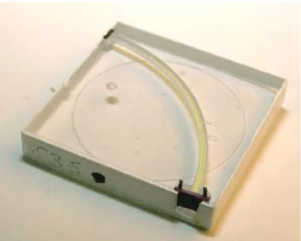
At the moment a test calorimeter of 1 m³size has been built and is currently being studied in test beam experiments by the CALICE collaboration (CAlorimeter for the LInear Collider with Electrons) [col, BDE⁺07]. The tiles are built from plastic scintillator which emits blue scintillation light. A curved groove is milled in the scintillator to install a wavelength shifting fiber inside (see figure 3.6). This fiber has the main task to convert blue light to green because the currently used SiPMs are not blue sensitive. Another effect is that the fiber collects the photons. So the

(24)

Fig. 3.6: Scintillator tile with mounted SiPM

number of photons that reach the SiPM has only a small dependence on the position of the particle passage.

One of our goals is to use a new generation of blue sensitive SiPMs to get rid of the wavelength shifting fiber (WSF) and the costly process of milling and installing the fiber. Another problem is the positioning of the SiPM (1×1 mm²) on the fiber (1 mm in diameter) [GRO06b]. Small mismatches between the SiPM and the WSF have a big impact on the photon detection efficiency. A design without a wavelength shifting fiber is expected to reduce the positioning requirements.

(25)

4 Concept of the Silicon Photomultiplier

Silicon Photomultipliers are a recent development in photon detection devices.

They have the capability to detect single photons and a high gain in the order of 10⁶. Furthermore they are insensitive to high magnetic fields. In the following the operation concept of the SiPM is explained. The definitions of the measured parameters are given. Later the linearity of the SiPM response is discussed.

4.1 Operation Concept

A photodiode [SZE81] is a p-n-junction typically implemented in silicon. If an incident photon creates a electron-hole pair the electron and the hole travel in opposite dirctions along the field in the p-n-junction. The photocurrent through the photodiode is proportional to the number of photons. Applying a bias voltage to the photodiode increases the field in the p-n-juntion and reults in shorter pulse responses to light pulses.

If the bias voltage is increased the avalanche effect is introduced. The electron from the primary electron hole-pair is accelerated sufficiantly so that it can create secondary electron-hole pairs. Those secondary electrons can generate more electron-hole pairs which lead to an avalanche of electrons in the semiconductor.

The avalanche stops itself when all electrons leave the p-n-junction. The gain of the avalance photodiode (APD) [Ham04, SZE81] is very much dependent on the bias voltage.

The Geiger-mode operation is reached when the field gradient is increased even more. In the Geiger-mode also the holes are accelerated up to energies needed to create secondary electron-hole pairs. The bias voltage VB needed for this process to start is defined as breakdown voltage VBD. The so called Geiger discharge propagates in both directions along the electrical field and for this reason does not stop.

ASilicon Photomultiplier is an array of avalanche photodiodes operated at a bias voltageVB = 40−70 V in the Geiger-mode. The SiPM has been given different

19

(26)

Fig. 4.1: Schematic design of a SiPM pixel [RIS⁺08]

names by the various vendors. Hamamatsu [Ham08] calls this concept MPPC which is an abbreviation for Multi-Pixel Photon Counter. Other names exist but only SiPM and MPPC will be used throughout the diploma thesis. The SiPM is designed in such a way that electron-hole pairs created by incident photons drift to the high field region (the p⁺ −n⁺-junction in figure 4.1). When they reach the high field region the Geiger discharge is started. A gain in the order of 10⁶ can only be reached if the bias voltage is higher than the breakdown voltage of the SiPM. The excess in voltage is called over voltage VO. To be able to stop the Geiger discharge two modes of quenching have been developed. Passive quenching utilizes a quenching resistor connected in series to the high field region to reduce the effective potential at the high field region as the current rises while the Geiger discharge takes place. This shuts down the Geiger discharge because the voltage at the high field region drops below the breakdown voltageVBD. After the quenching the potential at the high field region starts to recover to its original value. This method is also called limited Geiger-mode. Active quenching uses a transistor to shutdown the current. All tested devices were passively quenched. As the Geiger discharge continues until it is quenched a SiPM pixel is not sensitive to the number of incident photons. To overcome this limitation one uses an array of SiPM pixels. As all these “photodiodes” are current sources they are connected in parallel in order to add up their signals. In this way a pixel array produces a single analog signal, proportional to the number of pixels hit.

(27)

4.2 Equivalent Circuit Diagram 21

4.2 Equivalent Circuit Diagram

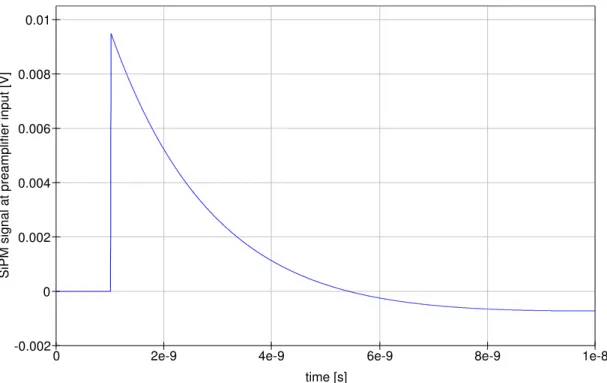
Figure 4.2 shows the equivalent circuit diagram of the SiPM. The sections below refer to the short hand notations introduced here. The capacities are important for the pulse shape and the recovery time of the SiPM. We also use this equivalent circuit diagram in section 5 to simulate the SiPM signal. The current source I1 substitues the high-field region. The quenching resistor R1 is connected in series to the the high-field region.

C1 C=50 fF P1

Num=1

C2 C=1 fF

P2 Num=2

R1

R=100 kOhm

C3 C=1 pF I1

I1=0 I2=0.1 A T1=1010 ps T2=1020 ps

Fig. 4.2: SiPM equivalent circuit diagram

4.3 Physical Effects

The following list shows the most important parameters of the SiPM. The technical terms explained here are used troughout the whole diploma thesis.

Gain

The gain of a SiPM is the charge amplification of the device. An incident photon creates a single electron-hole pair. The electron and the hole are amplified to 10⁵−10⁶ [Ham08] electrons and holes. The number of charge carriers can be determined from the charge contained in a SiPM pulse divided by the elementary charge. As electrons and holes are always generated in pairs the number of electrons is about half of the total number of measured charge carriers.

(28)

Fig. 4.3: Band struc- ture of silicon [SZE81]

Quantum efficency (QE)

The quantum efficency 0 ≤ QE ≤ 1 of a SiPM is defined as the probability that a single photon incident on the device generates a photocarrier pair that contributes to the detector current [ST91]. Figure 4.4 shows the later explained Particle Detection Efficiency (PDE). The PDE, however, is proportional to the QE. The avarage number (AN) of electron-hole pairs created by an incident photon is sometimes falsely referred to as the QE [Ott07, Ham08]. The AN is, however, an important number to calculate the QE. The average number of electron-hole pairs is very much dependent on the wavelength of the photon. Above the bandgap of silicon 1.1 eV the AN is about 1. Above 3.6 eV the AN rises above unity because impact ionization is possible (see figure 4.3). For even higher energies (UV light) the average number of charge carriers which contribute to the detector current starts to fall again, as the UV γs are absorbed before they reach the sensitive layer.

Photon detection efficency (PDE)

The photon detection efficency is usally referred to as a measure of the photon-sensitivity of the device (see figure 4.4)[Ham08]. It is given as a function of the wavelength of the incident photons. It depends on many parameters like back reflection from the silicon surface, the position of the electron-hole pair production and efficency to generate a breakdown (BE).

Most parameters have to be fixed at construction time, but at least the efficency to generate the breakdown can be controlled with the overvoltage.

In a first approximation the following formula can be used.

PDE = QE·BE·GF

The geometry factor (GF) is the ratio of the sensitive area to the whole

(29)

4.3 Physical Effects 23

Fig. 4.4: Particle Detection Efficiency of the Hamamatsu MPPCs [Ham08]

sensor area. It is decreased as the number of pixels in the array increases because of additional wires and resistors.

Thermal pulse

Thermally generated electron-hole pairs can fake a photon-generated Geiger-discharge. This happens statistically with a certain rate. This rate is exponentially increasing with the temperature. An increase in the over voltage also increases the thermal pulse rate rT P.

Afterpulse

The Geiger discharge generates electron-hole pairs. The number of electrons generated is approximately half the gain. Some electrons can be trapped in lattice defects. After a certain time the electrons can escape the trap by tunneling the potential barrier. The escaped electrons are accelerated in the electric field of the SiPM and can trigger a new Geiger discharge, which is then called afterpulse. The typical occurrance time of the afterpulses is different for every device type.

Dark pulse

When the SiPM is operated in a light tight box without illumination one can still observe a certain pulse rate. Usually this rate is generated by thermal pulses and their corresponding afterpulses. The sum of the rate from these two processes is called dark rate rD.

Recombination light

Electron-hole pairs in the avalanche can recombine and will emit photons.

The photons are emitted isotrophically. Their energies are in the order of the silicon bandgap 1.1 eV (see figure 4.3).

(30)

Crosstalk

Photons from the recombination light can trigger other pixels to fire as well.

Because of the short distances (10µ) between the pixels these two signals cannot be seperated by the test stand. The bandwidth and sampling rate of our setup limits us to 50 ps. In a real experiment the crosstalk is not desired, since it will spoil the energy measurement due to an additional contribution.

Recovery time

The recovery time tr of the SiPM is the rise time of the bias voltage after the quenching of the Geiger discharge. The rise timetr is given as the time the voltage needs to rise from 10% to 90% of its full value. The recovery time is typically much longer than the signal width. When loading the capacity of the SiPM, the quenching resistor and the capacity form an RC network. The recovery time can be calculated as tr ≈2.2·τ with the time constant τ = R₁C₂ of the RC network. The factor 2.2 is the conversion factor converting from the exponential charging of a capacitor exp _τ^t

to the 10-90 rise time tr. During the recovery the gain of this pixel is lower because it is proportional to the over voltage. This is seen by a shift to lower peak voltage values (see section 6.2). If the SiPM is hit by a small number of photons compaired to the number of pixels the effect of pixel recovery is small. The probability for a single pixel to be hit by at least one photon can be found in section 4.5.

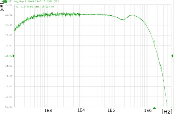
SiPM signal width

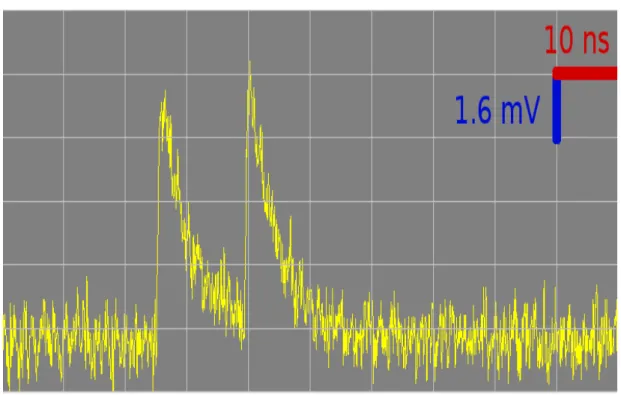
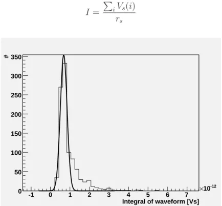
Usually the signal width is given by the full width half maximum (FWHM) of the signal (see figure 5.12). The rise and fall times of the SiPM are mainly given by its capacities and resistors because the amplification process itself is only few ps short [Rei08]. So the falling edge of the signal is an exponential characterised by the time constant τp = R₁C₃ (see figure 4.2). There is, however, a quenching effect which cuts off the waveform a few nano seconds after the pulse [Ott07]. This quenching is distributed randomly within a time window after the pulse as seen in figure 4.5. When integrating the signal this effect introduces additional variations to the common noise sources.

4.4 Time Distribution of Thermal- and Afterpulses

In the following a method for seperating thermal pulses from their afterpulses is introduced. For this, the statistical time distribution of the pulses is utilized. The formula for the time distribution is derived at the end of this section.

A Bernoulli experiment is composed of n experiments which have one of two outcomes with fixed probabilities p and (1 −p). A physical process of many

(31)

4.4 Time Distribution of Thermal- and Afterpulses 25

Fig. 4.5: Quenching of a typical SiPM single pixel [Ott07]

independent events can be described as a Bernoulli experiment if one can always find a time interval ∆t containing only one event or none. This is true for the thermal pulse rate of a SiPM. Afterpulses are triggered by trapped electrons which have a probability to tunnel their potential barrier. This process also leads to the statistics of the thermal pulse rate. Let the pulse rate beλ. Counting events from a Bernoulli experiment obeys Poisson statistics, which means that the number of counts k within a given time follows a Poissonian distribution.

Pλt(k) = (λt)^k k! e^−λt

The expectation valueN of the Poisson distribution is given by N =E(Pλt) = λt

with an error

hEi=√

λt=√ N

(32)

.

The two processes, thermal pulsesλT P and afterpulsesλAP, can only be separated if there are different pulse rates. In order to exploit this, one has to look into the distribution of the time intervals between consecutive pulses. Later on the mean time τ between pulses τ = _λ¹

is used.

The probability density to have two pulses within a time interval ∆t can be derived in this way:

The probability to have no event within ∆t is Pλt(0) = e^−λt. This probability must be equal to the probability that the event is going to occur after ∆t which is given by

Pλt = 1− Z ∞

∆t

f(t)dt

From this relation the unknown probability density function f(t) can be derived as

f(t) = λe^λt

The probability density functionf(t) multiplied with the number of time intervals recorded provides a distribution from which the fraction of afterpulses can be determined (see section 6.6).

The above calculation does not take into account that the afterpulses are dependent on prior after- or thermal pulses.

4.5 Response to Light Pulses and Dynamic Range

As the number of pixels in a SiPM is limited the response to a light pulse of arbitrary numbers of photons will not be proportional to the number of incident photons. We want to calculate the correct response in the following.

The average number of photo electrons in a SiPM array is determined by the number of photons in a pulse. This calculation neglects the possibility for some of the photons to hit the same pixel which will then only generate one Geiger discharge resulting in a decreased response signal. The effect of two photons hitting the same pixel is expected to be small when the number of pixels is large.

The following calculations are done for the ideal case. The probability to hit any of the SiPM pixels is 1. All SiPM pixels are equally probable to be hit. Crosstalk is neglected and the PDE is assumed to be 100%.

(33)

4.5 Response to Light Pulses and Dynamic Range 27 In a real experiment the illumination of the SiPM, e.g. with a laser spot, has to be considered. If not all pixels are exposed to light only the illuminated fraction of the pixels has to be taken into account. If the light spot is larger than the area of the SiPM one has to correct the result with the corresponding geometrical factor.

The question to be answered is the following [Cal08]: “How many pixelsk are hit on average byi incident photons when the total number of pixels is n?”

The probability not to hit a given pixel is q0 = 1− 1

n = n−1 n

The probability q for all our photons i not to hit this given pixel is q0 to the power of i

q =

n−1 n

i

The eventp complementary to q can be formulated as follows:

What is the probabilityp that a given pixel is hit by one or more photons?

This is calculated as follows:

p= 1−q = 1−

n−1 n

i

The expectation value for the average numberk of pixels fired for a given number of incident photons iis:

hki=n·p=n·

"

1−

n−1 n

i#

The result can be rewritten as:

hki=n·

1−exp

i·lnn−1 n

(4.1) To convince oneself about the correctness of the formula 4.1, some limits of the formula can be checked. The limits return sensible results:

limi→1hki= 1

(34)

i→∞limhki=n limi→0hki= 0

Another way of calculating the expectation value hki is by using combinatorics without the use of the complementary event. The calculations can be found in the appendix and only the results are presented here [Neu08].

The probability p(n, k, i) to hit k pixels with iphotons is:

p(n, k, i) = 1 nⁱ

"

n k

X

g1+...+gk=i

i!

g₁!·. . .·gk!

#

This is the sum over all combinations of g which sum up to i. The expectation value is given by

hki=

i

X

k=1

p(n, k, i)·k (4.2)

The expectation value in eq. 4.2 is calculated numerically and fitted with the a(1−exp(−bi)) ansatz (see figure 4.6). The data shown in this figure 4.6 is limited to a small number of pixels because of the quadratic increase of calculation time with the number of pixels.

/ ndf

χ2 1.549e-08 / 36 p0 37 ± 1.2

# of incoming photons

0 5 10 15 20 25 30 35

# of pixels hit

0 2 4 6 8 10 12 14 16 18 20 22 24

/ ndf

χ2 1.549e-08 / 36 p0 37 ± 1.2

/ ndf

χ2 1.549e-08 / 36 p0 37 ± 1.2 Mean value of pixels hit

Fig. 4.6: Simulated response of a perfect 37 pixel SiPM device to a light pulse with a given number of photons

(35)

4.5 Response to Light Pulses and Dynamic Range 29 The value for the fit quality _ndf^χ² ≈10⁻⁹ is small which indicates a perfect fit. The formula commonly used in the literature [Ott07] is just an approximation. It can be derived from the exponential function given in equation 4.1, using

ln(1 +x)≈x as an approximation in the exponent. This results in:

hki=n·

1−expi·lnn−1 n

≈n·

1−exp−i n

This formula is a good approximation if the number of pixels is large.

Figure 4.7 shows the response of a ideal 1600 pixel SiPM to incident photons calculated using the exponential function in equation 4.1. It can be approximated by a linear response function only for very small numbers of photons. Figure 4.8 shows the calculated response divided by the linear response in percent (^k−hki_k ).

If e.g. not more then 10% deviation from a linear response can be tolerated the maximal number of photons in a pulse to achieve the 10% deviation can be looked up in figure 4.8. Another interesting option is to linearize the signal with the known response curve.