Digital Object Identifier (DOI) 10.1140/epjc/s2003-01147-y
P HYSICAL J OURNAL C
Relativistic resonances as non-orthogonal states in Hilbert space
W. Bluma, H. Sallerb
Max-Planck-Institut f¨ur Physik, Werner-Heisenberg-Institut, M¨unchen, Germany Received: 28 June 2002 / Revised version: 13 November 2002 /
Published online: 14 March 2003 – cSpringer-Verlag / Societ`a Italiana di Fisica 2003
Abstract. We analyze the energy-momentum properties of relativistic short-lived particles with the result that they are characterized by two 4-vectors: in addition to the familiar energy-momentum vector (timelike) there is an energy-momentum ‘spread vector’ (spacelike). The wave functions in space and time for unstable particles are constructed. For the relativistic properties of unstable states we refer to Wigner’s method of Poincar´e group representations that are induced by representations of the space-time translation and rotation groups. If stable particles, unstable particles and resonances are treated as elementary objects that are not fundamentally different one has to take into account that they will not generally be orthogonal to each other in their state space. The scalar product between a stable and an unstable state with otherwise identical properties is calculated in a particular Lorentz frame. The spin of an unstable particle is not infinitely sharp but has a ‘spin spread’ giving rise to ‘spin neighbors’. This opens the possibility of a non- zero scalar product between states with unequal spin. – A first practical application of non-orthogonal states is seen in diffraction dissociation reactions whose large cross-sections are attributed to interference of states that are ‘partially identical’.
1 Introduction
From an experimental point of view, stable and unstable particles are often treated alike; for example, in multi- particle reactions one measures the cross section for the production of aρ-meson or anN∗-resonance or a pion or a proton without regard to their lifetimes. There is no fun- damental difference between stable and unstable states – this is our perspective in the following article1. From an algebraic point of view, particle states are eigenvectors of a time translation operator (Hamiltonian). Hermitian Hamiltonians acting on a Hilbert space have real energy eigenvalues, and the eigenstates are orthogonal to each other. If the particle is unstable and therefore the eigen- valueE−iΓ/2 is complex (Γ >0), the Hamiltonian can no longer be Hermitian, and the eigenvectors do not have to be orthogonal to each other or to eigenvectors with real energy eigenvalues.
Such non-orthogonality would have striking con- sequences for the behavior of unstable particles (resonan- ces) in collisions insofar as their identity is involved. Two non-orthogonal states |1 and|2with 1|2 = 0 are ‘not entirely distinguishable’ but have a ‘partial identity’ pro- portional to their scalar product1|2.
a e-mail: walter.blum@cern.ch
b e-mail: hns@mppmu.mpg.de
1 Although we think of particles and resonances as entities to be measured and of states as representing them mathemat- ically, we use these concepts without clearly distinguishing be- tween them
A first category of interactions where we expect mea- surable effects, is quasidiffractive scattering. These pro- cesses are similar to elastic scattering like
π−+p−→π−+p
p+p−→p+p, (1.1)
but one of the incoming particles is excited to a short-lived state with the same charge-like quantum numbers; it sub- sequently decays into several decay products. Examples are
π−+p−→A1+p (A1−→ρπ−→πππ)
p+p−→N1400∗ +p (N1400∗ −→pπ or pππ). (1.2) Such reactions have been measured and investigated in detail since the 1970’s [1]. They have exceedingly high cross-sections which vary only slowly with the energy of the collision. This behavior is shared between the reactions of groups (1.1) and (1.2).
In order to understand their similarity we note that elastic scattering proper (1.1) is governed by the phe- nomenon of quantum mechanical interference of the in- coming with the outgoing state, on account of their iden- tity. We will argue that such interference is also taking place in reactions (1.2), albeit on a reduced scale; this we call the partial identity of the (incoming) particle and the (outgoing) excited state. We propose that such partial identity is intimately connected with the short lifetime of the excited state, provided its charge-like quantum num- bers are the same.
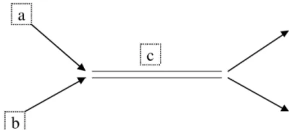
Fig. 1. Creation of a free unstable particle or resonance cin coproduction with other particles
If this is to succeed we will eventually have to include the spin of the unstable particle because quasidiffractive scattering is also observed when the excitation is to a dif- ferent spin. In fact we will argue that relativistic states with different spins also have a non-zero scalar product between each other if one of them is short lived.
In the quantum mechanical formalism, an unstable de- caying state (‘Gamov state’) is characterized by an en- ergy widthΓ >0, leading to a damped behavior in time e−i(E−iΓ2)t. If particles and states are considered in a spe- cial relativistic framework, the energy is part of an energy- momentum vector in Minkowski space. What then hap- pens with the energy width for a relativistic resonance, how does it have to be implemented in a Lorentz transfor- mation compatible framework, do we have to talk about a momentum width too?
Massive stable particles are characterized by the trans- lation and rotation eigenvalues of mass and spin. In a rel- ativistic framework the spin determining rotation group comes as part of the Lorentz group. What about a spin- ning unstable particle – do we have to introduce also some sort of a spin width?
In the following we draw out the main lines of an an- swer to these questions. We begin with a kinematic anal- ysis of relativistic unstable states (resonances)2. With re- spect to the possible spreads in energy, momentum and spin we employ Wigner’s method of Poincar´e group repre- sentations as induced by representations of the space-time translation and rotation groups. This method is prepared in Section 3 in the context of stable particles in such a way that it can be taken over and used to describe unstable particles. The first steps are done in Section 4, where we find a relativistically compatible wave function in space and time.
With it, the non-orthogonality between states one of which is unstable can be calculated for a specific Lorentz frame (Sect. 4.2). Their scalar product 1|2 is given by their overlap integral in space; instead of a delta distri- bution we find a function of their momentum difference which is widened by the momentum spread. The Lorentz compatible most general case is not yet treated.
Finally, in Section 5, we describe the appearance of a phenomenon which we call ‘spin spread’. The spin of a
2 We presented momentum and spin spread on the yearly
‘Workshop on Resonances and Time Asymmetric Quantum Theory’ in Clausthal-Zellerfeld (Germany), 6 to 10 August, 2000 (unpublished)
Fig. 2. Production of a resonancecbetween particlesaandb by external variation of the energy of (a, b)
short-lived state cannot be infinitely sharp, and we present a formalism to describe the appearance of ‘spin neighbors’
different by 1 unit from the original spin value. This opens the possibility for two states with unequal spin to be non- orthogonal to each other.
2 Energy-momentum properties of unstable particles
The two types of reactions that can produce a free unsta- ble particlec are ‘production’ (2.1) and ‘decay’ (2.2)
a+b−→c+d+e+· · · (c−→x+y+z+· · ·) (2.1) a−→b+c (c−→x+y+z+· · ·) (2.2) In terms of the kinematic variables of particle c we may describe the most general condition of its birth by the two-body reaction
a+b−→c+d (c−→x+y+z+· · ·) (2.3) where d represents the energy-momentum sum of all the other particles produced in the same reaction and assumed to be stable.
The situation we describe with reaction (2.3) is a free unstable particle produced as one entity (Fig. 1), in con- trast to an intermediate state which is produced in parts by varying at will the energy of the incoming particles a and b through a resonance energy at which their cross section typically goes through a maximum (Fig. 2).
2.1 Centre of mass system of the production reaction After specifying the total energy√
s, the masses mc and md as well as the decay width Γ of particle c, we may calculate in the centre of mass system of reaction (2.3) the energy Ec and the momentum kc of particle c. The conservation laws determine them to be
Ec=√
s(1 +u−v)/2 kc=√
s
(1 +u−v)2−4u/2, (2.4) with the abbreviations u= m2c/s and v = m2d/s. If the mass mc does not have a sharp value but is statistically distributed around its central value mc with variation
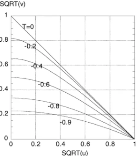
Fig. 3. Contours of constantT =δE/δk in theu-vplane in the centre of mass system of reaction (2.3). The physical region is the lower left hand triangle. T is seen to be in the interval
−1≤T ≤0 in die entire physical region
±δm, the ensuing variations inEc andkcare in first order ofδm3
δE=∂E
∂u du
dmδm=√
uδm (2.5)
δk=∂k
∂u du
dmδm= −1 +u−v (1 +u−v)2−4u
√uδm (2.6)
We note that the ratio δE/δk is always in the interval
−1 ≤ δE/δk < 0 because the domain of u and v is re- stricted to 0< u <1, 0≤v <1, |√
u|+|√ v|<1.
In Fig. 3 theu-v-plane is shown with contours of con- stantδE/δk, also calledT, derived from (2.5), (2.6). It is interesting to note that the value of T, which describes how the uncertainty ofmpropagates into energy and mo- mentum, depends on the overall reaction as well as on the unstable particle itself. It is easy to see from (2.4) to (2.6) that T is equal to the velocity of particle d, the energy- momentum sum of all the reaction partners of the unstable particlec. This holds for the moment in the centre of mass of the production reaction but can be generalized.
For the exponential decay a Breit-Wigner form formc
is appropriate, and the width of the distribution is given byδm=Γ/2. The corresponding widths ofE andkare
∆E =√
uΓ/2 (2.7)
∆k= −1 +u−v (1 +u−v)2−4u
√uΓ/2. (2.8)
We call them energy- and momentum-spread.
2.2 Lorentz-boost along the direction of motion If a particle characterized by (E, k, ∆E, ∆k) is Lorentz- boosted along its direction of motion, using the velocity
3 The index c is omitted from here onwards
β andγ2= 1/(1−β2), the values in the new system are given by
E
k
=γ
1 β β 1
E k
(2.9)
∆E
∆k
=γ
1 β β 1
∆E
∆k
(2.10) The widths (∆E, ∆k) transform exactly as the energy- momentum (E, k). The variableT =∆E/∆k transforms as
T= T+β
T β+ 1, (2.11)
it can reach all values in the interval −1 ≤ T < 1 even though it was restricted to the interval−1≤T <0 in the centre of mass system of reaction (2.3).
The invariants of the Lorentz-boost are (E, k)2= E2−k2=m2
(∆E, ∆k)2= (∆E)2−(∆k)2=−B2 (2.12) (E, k)(∆E, ∆k) = E∆E−k∆k=mΓ/2
The third relation in (2.12) is best evaluated in the rest system of the unstable particle wherek= 0 andE=m. In the second relation we have introduced B (capital beta);
the decaying state is characterized by both Γ and B. It turns out that (∆E, ∆k) is spacelike. One verifies this in the centre of mass system of reaction (2.3):
−B2= (∆E)2−(∆k)2
= −4uv
(1 +u−v)2−4u Γ2
4 ≤0 (2.13) In a diagramE vs. ka stable particle with rest massm is located on the hyperbolaE=
(k2+m2) throughE= matk= 0 (Fig. 4). If this particle is unstable so that its mass is distributed aroundmwith widthΓ one may draw two additional hyperbolas through E =m±Γ/2 at k = 0. The unstable state is characterized by a small vector (∆E, ∆k) at (E, k) connecting the two outer hyperbolas, the slope not exceeding 1. This restriction is a consequence of the spacelike nature of (∆E, ∆k). The unstable particle is measured as a statistical ensemble of individual events.
Each individual event is represented as a point along the small vector. There is a complete correlation between the deviations from the mean in E and the deviations from the mean ink.
2.3 Interpretation and examples
In the rest system (*) of the unstable particle whereE∗= m, k∗= 0, ∆E∗=Γ/2 this means especially that|∆k∗|is at least as large as Γ/2. The different parts of the mass distribution are not all at rest; when the centre is at rest
Fig. 4. An unstable particle in the energy-momentum plane is characterized by a straight line through the point (E, k) on the hyperbola (m), the relation between ∆E, ∆k and Γ is displayed
Table 1.Values assumed by the two 4-vectors in the two spe- cial Lorentz frames
4-vector Central rest system Sharp energy system
(E, k) (m,0) m
1 +4BΓ22,2BΓ (∆E, ∆k) Γ2
1,−
1 +4BΓ22
(0,−B)
the two wings fly apart in opposite directions. One may say that an unstable particle cannot come entirely to rest.
The consequences for the spin of unstable particles are discussed further down. The velocities involved are of the order ofΓ/mtimes the speed of light, which can be read off Fig. 4.
The value of∆k∗can also be calculated directly from (2.7), (2.8) and (2.10) by applying a boost back into the rest system of the unstable particle (velocity β =−k/E, (2.4)):
∆k∗=βγ∆E+γ∆k=−k
m∆E+ E
m∆k (2.14)
= −1 +u+v (1 +u−v)2−4u
Γ
2 (2.15)
The existence of the two fourvectors gives rise to two special Lorentz frames, one in which the average momen- tumk= 0, we call it ‘the central rest system’ of the un- stable particle, and one in which ∆E = 0; this we call
‘the sharp energy system’ of the unstable particle. Here we have added ‘central’ to the familiar name of ‘rest sys- tem’ because of the peculiar situation that the particles in the statistical ensemble that makes up the resonance can not all be simultaneously at rest. Table 1 summarizes the values of the two 4-vectors in these two systems.
The following examples illustrate the different values of ∆E/∆k and B2 as functions of the way the unstable state is produced. A ρ-meson (m = 0.77 GeV/c2, Γ =
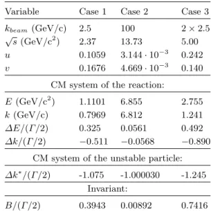
Table 2. Numerical values of some relevant variables for the three examples quoted in the text
Variable Case 1 Case 2 Case 3
kbeam (GeV/c) 2.5 100 2×2.5
√s(GeV/c2) 2.37 13.73 5.00 u 0.1059 3.144·10−3 0.242 v 0.1676 4.669·10−3 0.140
CM system of the reaction:
E (GeV/c2) 1.1101 6.855 2.755
k(GeV/c) 0.7969 6.812 1.241
∆E/(Γ/2) 0.325 0.0561 0.492
∆k/(Γ/2) −0.511 −0.0568 −0.890 CM system of the unstable particle:
∆k∗/(Γ/2) -1.075 -1.000030 -1.245 Invariant:
B/(Γ/2) 0.3943 0.00892 0.7416
0.15 GeV/c2) is produced by aπ-meson beam on a hydro- gen target in the forward direction:π+p−→ρ+p. In a first case the beam momentum kbeam is 2.5 GeV/c, in a second casekbeam= 100 GeV/c. The third case is a stable D+(1869 MeV/c2) and an unstable D∗−(2460 MeV/c2, Γ = 25 MeV/c2), produced as a pair in e+e−annihilation at√
s= 5 GeV/c2. We quote in Table 2 numerical values of relevant variables for these cases.
Another possible reaction is a nucleus decaying from some metastable state 1 into a state 2 with very short lifetime (1/Γ) by the emission of a light particle. If one identifies√
swith the mass of state 1, uwith the square of the mass of state 2 overs(uclose to 1), and neglecting the mass of the light particle (v= 0) we find B2= 0 and
∆k∗=−Γ/2 using (2.13) and (2.15).
2.4 Lorentz-boost in an arbitrary direction
Up to here the uncertainty ∆k in momentum was along the direction of motion. Now we want to apply a Lorentz transformation with velocity −→
β along a different, arbi- trary direction. Let −→
β have an angle θ with −→
k and let
−→∆kbe parallel to−→
k. Expressing the components along−→ β bykcosθand∆kcosθ, and the components transverse to
−→
β byksinθ and∆ksinθ, the kinematic variables of the unstable particle E,−→
k , ∆E,−→
∆k = (∆k/k)−→
k transform from the rest system of (2.3) into the primed system as follows:
E =γE+βγkcosθ;
kcosθ =βγE+γkcosθ; (2.16) ksinθ =ksinθ;
∆E =γ∆E+βγ∆kcosθ;
∆kcosΘ =βγ∆E+γ∆kcosθ; (2.17)
∆ksinΘ =∆ksinθ, where β =|−→
β| and γ2 = 1/(1−β2). In the primed sys- tem, the angle of the 3-momentum vector−→
k is denoted by θ, whereas the angle of the momentum uncertainty−→
∆k against−→
β is denoted byΘ. These two angles will be dif- ferent unless sinθvanishes: dividing the last two equations in each group, the transformed angles are given by
tanθ= 1 γ
sinθ
βEk + cosθ (2.18) tanΘ= 1
γ
sinθ
β∆E∆k + cosθ (2.19) These two expressions are not the same because the ratio E/k of the timelike vector (E,−→
k) is > 1 whereas the ratio∆E/∆k of the spacelike vector (∆E,−→
∆k) is<1. We conclude that in the general case the two vectors−→
k and
−→∆k will no longer be parallel but may in principle have any angle between them.
The situation described with the two variablesE and
∆kin Sects. 2.1, 2.2 and 2.3 reveals itself as a special case of a 4-vector (∆E,−→
∆k) where−→
∆kremained parallel to−→ k, as long as one stayed in a special set of Lorentz systems.
These are defined as being connected to the centre-of-mass system of the production reaction by a boost along the direction of motion of the unstable particle.
The most general case of a spread vector (∆E,−→
∆k) is given by 4 numbers which describe the complete correla- tion between the deviation of the individual particles of the ensemble from their mean values ofE, kx, ky,andkz.
3 Stable states
In this section we determine the relativistically compati- ble wave function for a stable particle from its Feynman propagator.
3.1 Wave functions for stable scattering states in quantum mechanics
The time behavior of a stable energy eigenstate in quan- tum mechanics is described by a U(1)-representation of the time translations R
representation: Rt−→e−iEt∈U(1)
ψ(t) = e−iEt|ψwith energyE∈R (3.1) The free scattering states with momentum−→
k can be built - with the position space orbits in the Schr¨odinger picture |ψ ∼= ψ(−→x) - by plane waves e−i−→k−→x which, by themselves, are no Hilbert states - only their packets d3ke−i−→k−→xµ(−→
k) which use square integrable momen- tum functions
d3k|µ(−→
k)|2 <∞. For a constant poten- tial V0, energy and the momentum of a scattering state are related as follows
−→k2
2 =E−V0 (3.2)
In polar coordinates for a radial symmetric dynam- ics (angular momentum invariant Hamiltonian [−→L, H] = 0) the scattering states are built by packets of spheri- cal Bessel waves jL for the Hilbert space with the radial translationsr∈R+functions for each angular momentum eigenvalueL= 0,1, . . .. The spherical Bessel functions [6]
are definable as plane wave coefficients with respect to the sperical harmonics Y0L(θ, ϕ) =
1+2L
4π PL(cosθ) ei−→k−→x = eikrcosθ= eiRζ:jL(R) = 1
2iL 1
−1dζ PL(ζ)eiRζ
=RL(−1 R
d
dR)LsinR R
⇒ei−→q−→x = ∞ L=0
iLjL(qr) (1 + 2L)PL(cosθ) (3.3) Time reversal, implemented by t ↔ −t and number conjugation α ↔ α, relate to each other the conjugated Hankel waves in the standing Bessel waves
jL= h+L−h−L
2i , h±L(R) =RL(−R1dRd )Le±iR
R (3.4)
They are the in- and outcoming waves with the large dis- tance behavior reflecting the large time (future and past) behavior
R→ ∞:
jL(R) →sin(R−RLπ2 ), standing waves h±L(R)→(∓i)Le±iRR ,
in- and outgoing waves
(3.5)
3.2 Energy-momentum and spin in Minkowski space Special relativity is characterized by the Poincar´e group SO0(1,3)−→× R4 as semidirect product of the orthochro- nous Lorentz group SO0(1,3) acting on the spacetime translations (Minkowski space) x ∈ R4 and on its dual space, the translation eigenvalues q ∈ R4, which consti- tute the energy-momentum space.
As first realized by Wigner, particles can be classified according to the stability group for their causal energy- momenta, i.e. for q ∈ R4 with q2 = m2 ≥ 0. Strictly positive mass particles,m2>0, e.g. electrons, have trans- formation properties with respect to spinSU(2). Massless particles,m2= 0, e.g. photons, are characterized with re- spect to the spin subgroup polarizationSO(2).
In the following we will restrict ourselves to massive particles, i.e. to an embedding of the spin group SU(2), the double cover4 of the rotation group SO(3) ∼= SU(2)/{±12}, into the real 6-dimensional groupSL( IC2), the double cover of the orthochronous Lorentz group SO0(1,3)∼=SL( IC2)/{±12}. For a relativistically compat- ible description, the nonrelativistic direct product group
4 In the following, both SO(3) and SU(2) will be called - somewhat sloppily - both spin and rotation group, and both SO0(1,3) andSL( IC2) come under the name of Lorentz group
with the rotations and the time translations is embedded [5] as a subgroup of the semidirect Poincar´e group
SO(3)×R→SO0(1,3)−→×R4
SU(2)×R→SL( IC2)−→×R4 (3.6) With respect to the translation subgroups, the unitary representations of the time translations are characterized by energiesE ∈R, and the ones of spacetime translations by energy-momentaq∈R4:
Rt−→e−iEt∈U(1), R4x−→e−iqx∈U(1) (3.7) With respect to the homogeneous subgroups: Halfin- teger and integer spin numbers S characterize the irre- ducible unitary representation of the spin group
DS :SU(2)−→SU(1 + 2S)⊂GL( IC1+2S), (3.8) whereas the finite dimensional irreducible representations of the Lorentz group - which, if nontrivial, are non-unitary - come with halfinteger and integer ’left-right spin’ num- bers [L|R]
D[L|R] :SL( IC2) (3.9)
−→SL( IC(1+2L)(1+2R))⊂GL( IC(1+2L)(1+2R)) The relativistically compatible embedding of a stable particle with spin-mass (S, m), characterized in its rest system by a spinSU(2) and time translationRrepresen- tation in the unitary groupU(1)◦SU(1+2S) of a complex (1 + 2S)-dimensional vector space
SU(2)×R(u= ei−→α−→σ /2, t)
−→DS(u)×e−imt∈U(1 + 2S) (3.10) is given by
SU(2)×R(S, m)→([L|R];q)∈SL( IC2)−→×R4 S, L, R∈ {0,1
2,1, . . .), q2=m2>0. (3.11) The relation of spinS to Lorentz{L, R}will be discussed below.
3.3 Representations of spacetime translations
The embedding of the unitary representations of the time translations for an energyE2=m2into a the unitary rep- resentations of the spacetime translations for energy-mo- mentum q2 =m2 is characterizable with the generalized functions
δ(E2−m2)→δ(q2−m2) (3.12) The unitary time translation matrix elements from t −→ eitm ∈ U(1) can be written as supported by an
energy distribution costm
−isintm
=
dE (m) m
E
δ(E2−m2)e−tiE
=
dE (E) E
m
δ(E2−m2)e−tiE
=−(t) dE
iπ 1 EP2−m2
E m
e−tiE
(3.13)
Here complex distributions are involved with a Dirac func- tion as real part and a principal value distribution as imag- inary part (integration with positiveo, then limito→0) a∈R, ±iπ1 a∓io1 =δ(a)±iπ1 a1P (3.14) and the step functions
a∈R,
ϑ(a) +ϑ(−a) = 1
ϑ(a)−ϑ(−a) =(a) =|a|a (3.15) The time representation matrix elements are embed- dable with an energy-momentum mass hyperboloid
Rm →q= (qj)j=0,1,2,3∈R4withq2=m2 (3.16) in two ways
dt
costm sintm
=m −
sintm costm
→
∂j
C(x|m) Sj(x|m)
=m
−Sj(x|m) C(x|m)
∂j
cj(x|m) s(x|m)
=m
−s(x|m) cj(x|m)
(3.17)
The boldface symbols with two arguments for transla- tions and eigenvalue, e.g. C(x|m), embed the trigono- metric functions with the corresponding notation for time translations and energy eigenvalue, e.g. costm.
Both embeddings come with a Lorentz scalar and a Lorentz vector: One embedding (Lorentz scalar cosine and vector sine) involves the functions
C(x|m)
−iSj(x|m)
=
d4q (2π)3(m)
m qj
δ(q2−m2)e−iqx (3.18) which occur as Fock state functions for relativistic particle fields (next subsection). The other embedding (Lorentz scalar sine and vector cosine) with an ordered Dirac ener- gy-momentum measure
cj(x|m)
−is(x|m)
=
d4q (2π)3(q0)
qj
m
δ(q2−m2)e−iqx
=−(x0)
d4q iπ(2π)3
qj
m
1
qP2−m2e−iqx(3.19) defines distributions which occur for the relativistic field quantization. The ordered Lebesque measure d4q(q0)ϑ(q2) leads to causal support
cj(x|m) s(x|m)
= 0 forx2<0 (3.20)
All those embeddings, (C,Sj) and (cj,s), are
‘on-shell’, i.e. energy-momentum supported byq02−−→q2= m2. They are matrix elements of spacetime translation representations in unitary Poincar´e group representations.
The cross over sums are used in Feynman propaga- tors for relativistic quantum particle fields and embed the causal time representations
e∓i|tm|=C(x|m)∓(x0m)is(x|m)
= d4q
(2π)3ϑ(±x0q0)2|m|δ(q2−m2)e−iqx
=∓ d4q iπ(2π)3
|m|
q2±io−m2e−iqx
(3.21)
As visible in the last line, Feynman propagators are sup- ported also ‘off-shell’, i.e. forq20− −→q2=m2(’virtual par- ticles’).
The embedding of the nonrelativistic in- and outgoing wave functions of the foregoing subsection
ψL±(t,−→x) = e−iEtkh±L(kr)YLm(θ, ϕ), withk=
2(E−V0) e.g.ψ0±(t,−→x) = e−iEte±ikr
r , ψ1±(t,−→x)
= e−iEt1∓ikr kr
e±ikr r
× 3
4π
∓√12sinθe±iϕ cosθ
, . . . (3.22) is seen explicitly in the harmonic analysis with respect to time and position space translations. In the scalar cosine of Minkowski spacetime the time representations come with standingL= 0 spherical waves as position realizations, if the energyq0 surpasses the mass thresholdm
C(x|m)
|m| =
d4q
(2π)3δ(q2−m2)e−iqx (3.23)
=−1 r
d dr
d2q
(2π)2δ(q2−m2)e−iqx|x=(t,r)
=
dq0
(2π)2ϑ(q20−m2)e−iq0tsinr
q20−m2 r
For Lorentz scalar integrands, the 2-sphere integration (polar coordinates with r = |−→x|) over the 2-sphere SO(3)/SO(2) goes over from the Lorentz groupSO0(1,3) to an abelian noncompact subgroupSO0(1,1) with trivial spin. It yields the characteristic 2-sphere distribution fac- tor 1
r (Kepler factor). For the Lorentz groupSO0(1,1) in two spacetime dimensions the integralsd2q=dq0dq3both over the energyq0 and the directed momentum modulus q3=(q3)|−→q|go over the full real axis ∞
−∞.
The harmonic analysis of both the scalar sine and the ordered scalar sine displays irreducible time representa- tions multiplied with spherical waves for energiesq20 over the thresholdm2 (on shell). The off shell contributions of the ordered sine for q20 smaller than m2 give irreducible time representations, multiplied with a Yukawa potential
1 (x0)
is(x|m) m
=− d4q
(2π)3
(q0)δ(q2−m2)
−πi−q21
P+m2
e−iqx
= 1 r
d dr
d2q (2π)2
(q0)δ(q2−m2)
−πi−q21
P+m2
e−iqx|x=(t,r)
=
dq0
i(2π)2e−iq0t
ϑ(q02−m2)
−(q0)isinr
q2 0−m2 r cosr
q2 0−m2 r
+ϑ(m2−q02) 0
e−r m2−q2 r 0
(3.24) The harmonic analysis of the Feynman propagator contains the sum of an ‘on shell’ particle with spherical wave, in- or outgoing as determined by±ioresp., and an
‘off shell’ Yukawa interaction
∓
d4q iπ(2π)3
1
q2±io−m2e−iqx
=±1 r
d dr
d2q iπ(2π)2
1
q2±io−m2e−iqx|x=(t,r)
=±
dq0
i(2π)2e−iq0t
ϑ(q02−m2)e±ir
√q02−m2
r +ϑ(m2−q02)e−r
√m2−q02
r
(3.25)
3.4 Relativistic wave functions for spinless stable particles
The matrix elements of unitary spacetime translation rep- resentations of the foregoing subsection arise for a massive spinless particle, e.g. theπ0-meson, considered as stable.
A relativistic hermitian scalar Bose fieldA(x) for such a particle has the harmonic decomposition into translation eigenvectors, called creation operators u(−→q) and annihi- lation operators u (−→q) for momentum−→q
A(x) = d3q q0(2π)3
e−iqxu(−→q)+e√ iqxu(−→q) 2
withq= (q0,−→q), q0=
m2+−→q2 (3.26) As indexed by the momenta −→q ∈R3, the associate state space is overcountably infinite dimensional.
The basic vectors have as commutators (quantization) and as Fock state value for anticommutators (denoted with. . .F)
[u (−→p),u(−→q)] = (2π)3q0δ(−→q − −→p) {u (−→p),u(−→q)}F =u(−→p)|u(−→q)= (2π)3q0δ(−→q − −→p) (3.27) With the shorthand notation for translation dependent (anti) commutators of spacetime dependent operators
=±1 : [A, B](x) = [A(x2), B(x1)]
=A(x2)B(x1) +B(x1)A(x2) for allx=x1−x2 (3.28)
the Feynman propagator sums up the on-shell Fock value of the quantization opposite anticommutator and the on- and off-shell causally ordered quantization commutator
{A,A}(x)−(x0)[A,A](x)F
=C(x|m)−(x0)is(x|m) m
=−
d4q iπ(2π)3
1
q2+io−m2eiqx (3.29) The wave function for an outgoing scalar particle (de- noted with the corresponding non-boldface letter – here A for the particle field A), considered from a reference system wherein the particle has energy q0 =E > m can be obtained by Dirac-picking with δ(q0−E) in the har- monic expansion of the Feynman propagator above the corresponding contribution with the angular momentum L= 0 outgoing Hankel wave (an irrelevant normalization factor i
(2π)2 is omitted) A(t, r) =−
d4q 2π2
1
q2+io−m2e−iqxδ(q0−E)
= e−iEteikr r
= e−iEt kh+0(kr) withk=
E2−m2 (3.30)
Summarizing, the relativistic wave function for an outgo- ing scalar particle is
A(t, r) = e−iEt eikr
r (3.31)
In the rest system of the particle, denoted by the sup- script =, one obtains the product of the time orbit withrs the Kepler 2-sphere distribution factor
(E, k)= (rs m,0)⇒A(t, r)=rs e−imt
r (3.32)
4 Unstable states
4.1 Construction of the wave function
Our starting point is (3.30) where the wave function for a stable particle of a given energy E > m was obtained from the harmonic expansion of the Feynman propagator:
From the reservoir of all wave functions e−iqx one picks the one with energyE.
For an unstable particle we introduce two modifica- tions: Firstly the distributional ‘io’ in (3.30) is replaced by the invariant width ‘imΓ’. Obviously the stable parti- cle results have to reappear in the limitΓ →0.
Secondly,q0 is no longer fixed to be equal to E; the integration variables must be correlated in a different way.
In the simple case treated in Sects. 3.1 to 3.3 (−→
∆kparallel
to −→
k), bothk ≡ |−→
k|and ∆k≡ |−→∆k| are independent of direction, and the correlation is given by the expression
q0−E
|−→q| −k = ∆E
∆k Therefore we replace in (3.30)
δ(q0−E)→δ(C(q0−E)−S(|−→q| −k)) (4.1) where
C=±∆k/
(∆k)2−(∆E)2 S=±∆E/
(∆k)2−(∆E)2 (4.2) The normalization factor
(∆k)2−(∆E)2, or B (cf. (2.12)) was introduced because it guarantees that the case of∆E= 0 falls back into the old formδ(q0−E), and because it is Lorentz-invariant. The signs in (4.2) must be chosen such thatC >0.
Looking at the new δ-distribution (4.1), we observe that its argument may be interpreted as the energy com- ponent of a vector in an energy-momentum space spanned by the deviations (q0−E) and (|−→q| −k). In fact, the nor- malized coefficientsCandSmay be interpreted as coeffi- cients of a Lorentz boost
C= coshζ, S= sinhζ (4.3) from the general system in which the decaying particle has (E, k) and (∆E, ∆k) to the sharp energy system (primed variables) in which∆E= 0:
a b
=
C −S
−S C a b
(4.4)
for
a b
=
E k
,
∆E
∆k
,
t r
,
q0
Q
The variableζin the coefficients (4.2) is given in terms of the velocityβ of this boost as ζ= arctanhβ.
C(q0−E)−S(Q−k) =q0−E
E2−k2=E2−k2 (4.5) Et−kr=Et−kr
4.1.1 Harmonic analysis
In the sharp energy system (ses) the wave function for an unstable particle with energyE > mis
ψ(t, r)ses=− d4q
(2π)2
δ(q0−E)
q2−m2+imΓe−xiq
= e−iEteikr
r (4.6)
withΓ >0 and k=
k2+imΓ , wherek2=E2−m2. (4.7) The case of the general system requires the new Dirac delta function (4.1) in the Fourier integral. The integral is first solved in the sharp energy system (primed vari- ables), the result (4.8) is then Lorentz-transformed into the general system (unprimed variables).
ψ(t, r) =− d4q
(2π)2
δ(C(q0−E)−S(Q−k)) q2−m2+imΓ e−xiq
= e−iEteikr r
= e−iEteikr
r ei(k−k)r (4.8)
because of (4.5). Here k−k=
k2+imΓ −k which becomes imΓ/2 k
(4.9) to first order ofmΓ/k2. This dimensionless parameter is of the orderΓ/m1. Inserting (4.4) we find the factor
(k−k)r = imΓ/2
−SE+Ck(−St+Cr) (4.10) which, using (4.2) and (2.12), turns out to be −i∆Et+ i∆kr. Therefore the relativistic wave function of the un- stable state is
ψ(t, r) = e−i(E−i∆E)t ei(k−i∆k)r
r (4.11)
to first order ofΓ/m.
In the central rest frame (crs) the wave function takes the form
ψ(t, r)crs= e−i(m−iΓ/2)te−|∆k∗|r
r (4.12)
Note that∆k∗≤ −Γ/2<0 in the central rest frame of the decaying state. An unstable state unavoidably has some spatial extension.
If one does not want to go to the first order approx- imation in Γ/mone may define a complex constant η in (4.9)
k−k =
k2+imΓ −kdef= iηB (4.13) which is 1 in the first order ofΓ/m. It may be expressed in terms of a ratio of invariants of (2.12) and is
iη= mΓ/2 B2
1−
1 +i4B2 mΓ
(4.14) With it the wave function generally takes the form
ψ(t, r) = e−i(E−iη∆E)t ei(k−iη∆k)r
r (4.15)
Looking back at the integral (4.8), we see how theδ- function picks out the particular solution from the Lorentz-invariant reservoir of all possible solutions. We note that the variables E, k, ∆E, ∆kand their invariants m2, mΓ and B2 (c.f. (2.12)) fall into two categories. The first comprisesm2 andmΓ – they belong to the Lorentz- invariant part of the integrand (4.8) and are therefore a universal description of the unstable state, independent of a particular Lorentz frame or any particular production conditions. The second comprises the others,E, k, ∆E, ∆k and B – they appear in the δ-function of the integrand (4.8) and therefore describe the unstable state in the par- ticular conditions in which it was produced. There is an analogy with the spin of stable particles: the magnitude of spin is a universal property of the particle (mathemat- ically characterized by the dimension of the representa- tion space), the spin component is a particular property of the particle which depends on the production condi- tions (mathematically characterized by an eigenvector in the representation space).
A suitable notation would separate the two categories of variables. The unstable state, characterized by 4 real numbers, could be written as|m2, mΓ;k, ∆kor|m2, mΓ; E, ∆E, the universal variables to the left of the semikolon, the experiment-dependent to the right. The correspond- ing notation for a spin state (of a stable particle) would be |S;S3.
4.1.2 Comparison of (4.11) with the traditional ansatz Traditionally [2] [8] one describes a decaying state in its rest system with the ansatz
ψ(t, r)=rs 1
re−i(m−iΓ/2)t (4.16) If the state has energy-momentum (E, k), (4.16) is re- placed by
ψ(t, r) = e−i(E−i∆E)t ei(k−i∆k)r
r (4.17)
The imaginary parts traditionally also form an energy- momentum four-vector (∆E, ∆k) which is the result of the same Lorentz boost that transforms
(m,0)−→(E, k) Γ
2,0
−→(∆E, ∆k) = E
m Γ
2, k m
Γ 2
(4.18) The difference in the two approaches is in the norm of (∆E, ∆k); our spread vector is spacelike, the traditional one is timelike. The traditional spread vector keeps the same ratio of the momentum over the energy components in all Lorentz frames:
∆k
∆E
traditional
= k
E (4.19)
Traditionally, there is no sharp energy system, and the momentum spread in the particle’s rest frame is zero.