U N I V E R S I T Y OF D O R T M U N D
R E I H E C O M P U T A T I O N A L I N T E L L I G E N C E COLLABORATIVE RESEARCH CENTER 531
Design and Management of Complex Technical Processes and Systems by means of Computational Intelligence Methods
Time-Optimal Large View Visual Servoing with Dynamic Sets of SIFT
Thomas Nierobisch, Johannes Krettek, Umar Kahn and Frank Hoffmann
No. CI-227/07
Technical Report ISSN 1433-3325 February 2007
Secretary of the SFB 531 · University of Dortmund · Dept. of Computer Science/LS 2 44221 Dortmund · Germany
This work is a product of the Collaborative Research Center 531, “Computational
Intelligence,” at the University of Dortmund and was printed with financial support of
the Deutsche Forschungsgemeinschaft.
Time-Optimal Large View Visual Servoing with Dynamic Sets of SIFT Features
Thomas Nierobisch, Johannes Krettek, Umar Khan and Frank Hoffmann
Abstract — This paper presents a novel approach to large view visual servoing in the context of object manipulation. In many scenarios the features extracted in the reference pose are only perceivable across a limited region of the work space.
The limited visibility of features necessitates the introduction of additional intermediate reference views of the object and requires path planning in view space. In our scheme visual control is based on decoupled moments of SIFT-features, which are generic in the sense that the control operates with a dynamic set of feature correspondences rather than a static set of geometric features. The additional flexibility of dynamic feature sets enables flexible path planning in the image space and online selection of optimal reference views during servoing to the goal view. The time to convergence to the goal view is estimated by a neural network based on the residual feature error and the quality of the SIFT feature distribution. The transition among reference views occurs on the basis of this estimated cost which is evaluated online based on the current set of visible features. The dynamic switching scheme achieves robust and nearly time-optimal convergence of the visual control across the entire task space. The effectiveness and robustness of the scheme is confirmed in an experimental evaluation in a virtual reality simulation and on a real robot arm with a eye-in-hand configuration.
I. INTRODUCTION
Vision is expected to play a progressively more important role in service robotic applications in particular in the context of manipulation of daily life objects. Image based visual servoing solely relies on 2D image information for the alignment of the end-effector with an object of unknown pose [1]. The desired pose for grasping is demonstrated to the robot and a set of reference features is extracted from the image. Subsequent approaches of the robot and camera to the goal pose are accomplished by regulating the image error between the current and reference features without explicit geometric reconstruction of the object pose.
Optimal motion control for visual servoing to a static reference view has been discussed in [2], [3] and is based on the decoupling of the translational and rotational degrees of freedom achieved by a partial pose estimate using either the homography or the fundamental constraint. Both approaches require the online estimation of the homography or funda- mental matrix in the servo loop, with at least four or eight feature point correspondences. The method in [2], [3] focuses on the optimal control with respect to a fixed set of features, whereas our approach addresses the issue of large view visual servoing with extraction and matching of dynamic
T. Nierobisch, J. Krettek, U. Khan and F. Hoffmann are with the Faculty of Electrical Engineering and Information Technology, Chair for Control and Systems Engineering, Universit¨at Dortmund, 44221 Dortmund, Germany thomas.nierobisch@uni-dortmund.de
sets of SIFT features. The view space is partitioned by an entire set of intermediate, partially overlapping reference views of the object. The authors in [4] integrate a path planner in the image space with a visual controller based on potential fields in order to obtain visual navigation for large displacements. The work in [5] extends these concepts by qualitive visual servoing based on objective functions that capture the progression along the path, the feature visibility and camera orientation. This paper provides a contribution to optimal path planning in the image space considering the residual feature error in conjunction with the quality of the feature distributions in alternative reference views.
The additional flexibility of dynamic feature sets provides the basis for adaptive online switching among reference views while navigating towards the goal view. [6] describes a method for automatic selection of optimal image features for visual servoing in terms of robustness, uniqueness and completeness. Additional performance criteria concern the systems observability, controllability and sensitivity. Our vi- sual features are generic moments computed over a dynamic set of point features. Maximum robustness and observability of the statistical moments is achieved by aggregation over all extracted and matched features. Our objective is to estimate the quality of feature sets from alternative reference views online based on similar criteria as [6]. Optimal reference view selection relies on an estimate of the time to conver- gence of residual errors. This estimate is provided by a neural network that is trained with feature errors and distributions as input to predict the time to convergence. The proposed scheme is model-free in so far that it does not depend on a geometric object model or reconstruction of the object or camera pose, which means that navigation and control is entirely performed in the image space.
The paper is organized as follows: Section II provides the
definition of decoupled visual features based on weighted
moments of SIFT features used for visual servoing in 6 DOF,
followed by a stability analysis motivated by the feature
distribution in the image space. Due to the limited visibility
of SIFT features across different views it is necessary to
introduce intermediate reference views. The time optimal
reference selection to accomplish large view visual servoing
is introduced in III as well as the navigation in the image
space. Section IV demonstrates the experimental results
on a sphere and a semi cylinder setup and analyzes the
convergence behavior of alternative switching strategies. The
paper concludes with a summary and outlook on future work
in section V.
II. VISUAL SERVOING WITH SIFT FEATURES A. Decoupled visual features
Scale invariant feature transformations (SIFT) introduced by Lowe [7] occur frequently in textured objects and are invariant to changes in scale, orientation, illumination and affine transformations. They are uniquely identifiable and robustly matched across different views of the same object.
These properties render them particularly suitable for model free image based visual servoing.
Our scheme is motivated by the work of [8], which relies on image moments rather than points features to overcome the shortcomings of visual servoing schemes. SIFT features for visual servoing applications were first introduced by [9], in which the authors focus on the robust feature selection and explicitly reconstruct the object pose based on the epipolar geometry. A novel image-based controller that augments conventional point features by the additional attributes scale and keypoint orientation of SIFT features is presented in [10]. This work is improved by establishing a one-to-one correspondence between feature and camera motion based on weighted moments that eliminates or at least minimizes the undesired couplings [11]. A set of reference SIFT features is automatically extracted from an image of the object captured in the demonstrated reference pose. The automatic feature selection detailed in [10] identifies a subset of robust and non-ambiguous features for the ultimate visual servoing of the robot to the reference pose.
The visual servoing in 6 DOF relies on six associated statistical moments computed over the location, scale and orientation of the SIFT features. Notice, that the term feature has a dual meaning as it refers to the point like SIFT features as well as the visual features aggregated over a set of matched SIFT features subject to control. A single SIFT-feature F i contains four attributes, namely its pixel coordinates u i and v i , its canonical orientation φ i and its scale σ i . The scale changes inversely proportional to the distance between the camera and the object. The orientation φ i is consistent with the camera rotation about its optical axis.
Scale and orientation are ideal for the control of the distance to the object and the rotation around the optical axis as they prove widely independent of translations and rotations along the other axes. The rotation and translation along the cameras optical axis are captured by the moments
f γ = ∑ n i =1 φ i
n , f z = ∑ n i =1 σ i
n (1)
which correspond to the mean orientation and scale of detected SIFT-features. The translations along x- and y- axis are regulated with respect to the geometric centroid of the point features. The geometric centroid is susceptible to translations along the z-axis causing an undesired coupling with this motion. The decoupling of the centroid from the z- motion is achieved by dynamically weighting the individual point features. The moments
f x =
n
∑
i =1
w i u i , f y =
n
∑
i =1
w i v i (2)
correspond to the weighted mean of the matched SIFT feature locations and capture translations along the x- and y- axis respectively [11]. The 6 DOF visual control is completed by the moments
f α =
n− 1
∑
i =1 n
∑
j = i +1
(− v ˆ i − v ˆ j )·
~ p j −~ p i
∑ n k =1 ∑ n l = k +1 k~ p k − ~ p l k (3) associated with rotations along the x- and y- axis. The moments f α and f β detect the perspective distortions of lines connecting pairs of SIFT features caused by rotations.
The term
~ p j −~ p i
denotes the length of the line connec- ting the two pixels. This length is multiplied by the weight factor (− v ˆ i − v ˆ j ). Its sign indicates whether the line is above or below the u-scan-line through the cameras principal point. The absolute magnitude of the weight increases with the vertical distance from the image center. The moment represents the equivalent effect of dilations and compressions of lines caused by rotations along the y-axis. The moment f β is defined in an analog manner to f α , by interchanging the u and v components.
B. Local stability analysis
The local stability of the visual control loop requires that the feature error has a unique minimum at the reference pose.
Even though a single SIFT feature suffices in principle for coupled 4 DOF visual servoing, the computation of weighted centroids requires at least two non-coincident point features for decoupled 4 DOF visual servoing. Visual servoing in 6 DOF depends on at least three non-colinear SIFT features.
Convergence of the control to the reference pose is achieved under the assumption of continuous visibility and perceptibi- lity of this minimum number of correspondences. As stated in [6], three feature points which ideally form a large-area triangle enclosing the origin are optimal for visual control.
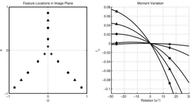
Three features are minimal as the distortion in features f α and f β is observed relative to the average length between the points. However, not all configurations of three feature points are suitable for control. Stable visual control of the rotations requires that the three features are widespread and that the formed triangle encloses the origin. A too small separation of the three point features causes a change of sign in the moments f α and f β resulting in an unstable control. Fig. 1 illustrates this phenomenon as it shows the point distributions for five triangular sets of different separation. The right part of figure depicts the corresponding variation of the moment f α for the five sets with respect to rotation about the x- axis. In case of the widespread feature set the feature error f α has a unique root at the origin. However, the feature set closest to the origin induces two roots of f α with non-zero rotational error to the left and right of the origin. These additional roots cause the visual control to converge to an equilibrium state that differs from the reference pose. Figure 2 shows the development of the feature-moment f x during a lateral movement for a randomly chosen subset of features.
The feature-configurations showed in the upper left resp.
lower right corner of the figure demonstrate the effect of
an extreme feature-occlusion on the calculated moment. The
−1 0 1
−1 0 1
Feature Locations in Image Plane
U
V
−30 −20 −10 0 10 20 30
−0.1
−0.08
−0.06
−0.04
−0.02 0 0.02 0.04 0.06 0.08
Moment Variation
Rotation [α°]
fα
Fig. 1. Feature distribution in the image plane and its impact on the rotation moments
configurations that are used for all other displayed moment- developments represent feature-occlusions with a randomly changing distribution in the image-plane as well as in the number of features. The camera is laterally displaced by -40 cm to 40 cm while the features at a distance of 75 cm are projected onto a normalized image-plane. The figure demonstrates the impact of SIFT-feature occlusions on the visual moment. The two envelopes marked by triangles and rectangles correspond to the extreme, but highly unlikely sce- nario in which all features in either the left or right half-plane are occluded resulting in a highly asymmetric configuration.
The dotted lines correspond to random feature occlusions. In all cases the unique equilibrium point is globally stable. In case of the two extreme distributions the weighted feature moment does not evolve monotonically with the lateral displacement, due to the effect of skewed weights which increase in absolute magnitude with the asymmetry of the feature distribution. Even though this phenomenon effects the rate of convergence global stability is still guaranteed.
−40 −30 −20 −10 0 10 20 30 40
−0.3
−0.2
−0.1 0 0.1 0.2 0.3
lateral displacement [cm]
resulting moment fx
+ +
+ +
+ + +
+ ++ + +
+ + +
+ +
+
+ ++
+
+ +
+ + +
+ u
u v v
Outmost left goal−view configuration
Outmost right goal−view configuration
∆
Fig. 2. Feature distribution in the image plane and its impact on the rotation moments
In contrast to [6] our approach does not select the subset of optimal features online, but rather utilizes all available features matched between the current and the reference view in order to maximize robustness and accuracy. The general definition of visual features in terms of statistical moments renders the scheme robust with respect to occlusion or partial
loss of perceptibility of features. Notice, that the reference features are recomputed online with respect to the subset of matched features. Typically, the number of matched features varies between 5 to 40 features, depending on the camera pose and the amount of useful texture in the current image.
The visibility of individual SIFT features is limited by the cameras field of view, occlusion through the object and changes in perspective. Therefore, large view visual servoing requires multiple reference images in order for the camera to navigate across the entire view hemisphere. Intermediate reference images are captured across the entire work space in x-, y- and z-direction. It is assumed that the object always remains in view of the camera, which naturally restricts the orientation of the camera along the x- and y-axis. Our point of departure is a set of overlapping intermediate reference views with partially shared SIFT features among neighboring images. The objective of our work is to generate a time optimal and robust visual control across the entire task space by proper switching among neighboring reference images.
For that purpose, the cost of the current view is compared with respect to all overlapping reference images, and the control switches to the reference image with minimal cost.
A crucial step is to estimate the cost in terms of the time to reach the reference pose from the feature error and geometric configuration of features. Based on the estimated cost the optimal path is determined by shortest path graph search.
III. TIME-OPTIMAL REFERENCE IMAGE SELECTION
For large view visual servoing intermediate views are defined to navigate across the entire view hemisphere. It becomes desirable to switch between intermediate views in a stable, robust and time-optimal manner. The cost in terms of number of control cycles to converge from the current view to the reference image is estimated in order to compute the optimal path. Crucial for this purpose is the proper definition of performance criteria for approximation of the cost function and the analysis of their correlation with the cost. In our case, an artificial neural network learns the relationship between the control criteria and the costs in a supervised manner.
The training data is obtained from observations of the actual number of control cycles required for transitions between neighboring reference views.
A. Control criteria
1) Feature error: The overall feature error f (I)={ ∆ f x , ∆ f y , ∆ f z , ∆ f α , ∆ f β , ∆ f γ }
constitutes the most significant performance criterion for the estimation of the cost.
A single feature error alone does not provide a good
estimate of cost, because the actual time until convergence
depends on the feature error with the slowest task space
motion, usually associated with the translational degrees of
freedom. The rotational errors are bounded by the visibility
constraint and are usually stabilized within a few control
steps. Each element of f (I) is normalized to the interval [0, 1]
according to its maximum range. The total feature error is the sum of normalized errors.
f ˆ (I) =
6
∑
i =1
f ˆ i (I)
(4) The feature error already attributes to a substantial amount of variation in the cost, nevertheless the cost estimate is improved by inclusion of additional criteria that capture the quality and robustness of visual control.
2) Number of correspondences: The robustness and the control performance increase significantly if more than the minimal number of correspondences is established. The red- undancy of multiple features reduces the noise level and con- tributes to the beneficial widespread dispersion of features in the image space. A small number of features might cause a compact distribution of point features, which as shown earlier causes poor or even unstable control in the image space. The number of matched features also provides an estimate of the geometric distance of the current view to the reference pose.
Distant poses only share a subset of mutually visible features, whereas the number of correspondences naturally increases with the proximity of both viewpoints. The criterion C(I) = n is defined as the absolute number of feature correspondences between the current and the reference view. The criterion
C n (I) =
0 n < n min n
n max n min < n < n max
1 n max < n
(5)
normalizes C(I) as it requires a minimal number of features n min and saturates at the upper limit n max = 40, at which em- pirically no further improvement of the control performance is observed. The parameter n max is independent of the object and not crucial for approximate cost estimation. The absolute number of visible features alone is not a unique indicator of the expected cost as it also depends on the distribution of these features defined in terms of their entropy and variance around the centroid.
3) Entropy: Entropy measures the order or disorder in a distribution. The image is partitioned into N = 10 vertical and horizontal equally spaced columns and rows. The entropy along the two axes is calculated as
E u (I) = −
N
∑
i =1
H u (i) · log N (H u (i)) (6) E v (I) = −
N
∑
i =1
H v (i) · log N (H v (i)) (7) in which H u (i) and H v (i) denote the relative frequency of SIFT features in the ith column respectively row.
The entropy assumes a value in the interval [0, 1], in which a high entropy indicates a uniform distribution. A low entropy reveals an inhomogeneous distribution, which harms the robustness and speed of convergence of visual servoing.
4) Centroid location: The visual features f α and f β require a distribution uniformly centered around the principal point in order to capture the distortion of line segments. The
deviation of the feature centroid from the origin is expressed by
| u| ¯ = ∑ n
i =1
| u i − n u 0 | | v| ¯ = ∑ n
i =1
| v i − n v 0 | (8) in which low values represent desirable feature distributions.
5) Variance of the feature distribution: The variance of the feature positions provides an additional estimate of the quality of the feature distribution. A low variance in particular in conjunction with a dislocated centroid reflects a feature distribution that is suboptimal for visual control and delays the convergence to the reference image. The variances are computed as
σ u =
n
∑
i =1
(u i − u) ¯ 2
n , σ v =
n
∑
i =1
(v i − v) ¯ 2
n (9)
Notice, that entropy reflects the geometric homogeneity of the feature set, whereas variance captures its width.
B. Correlation between performance criteria and time to convergence
Control experiments from 150 initial positions randomly distributed over the task space are recorded in order to eva- luate the correlation between the performance indicators and the time to convergence. Each control step of the individual runs constitutes a training sample for supervisory learning of the neural network. A control run is considered as suc- cessfully converged to the reference image if all image errors are reduced to within 10% of their average initial value. The correlation between the performance criteria and the actual time to convergence provides insight into the influence and relevance of the individual indicators. The linear dependency between two stochastic variables is computed according to Pearson’s correlation coefficient:
r XY =
n
∑
i =1
(x i − x)·(y ¯ i − y) ¯ r n
∑
i =1
(x i − x) ¯ 2 · r n
∑
i =1
(y i − y) ¯ 2
, (10)
which assumes values in the interval [−1, 1]. Large absolute values indicate strong correlation between the two quantities.
Table I specifies the correlations between the performance indicators and the cost in terms of time to convergence.
TABLE I
P EARSON CORRELATION BETWEEN PERFORMANCE FEATURE ERROR RESP . CRITERIA AND TIME TO CONVERGENCE
∆ f x ∆ f y ∆ f z ∆ f α ∆ f β ∆ f γ f ˆ r XY 0,30 0,14 0,17 0,14 0,13 0,13 0,63
C(I) C n (I) E u (I) E v (I) | u| ¯ | v| ¯ σ u σ v r XY -0,66 -0,72 -0,66 -0,72 0,44 0,32 -0,64 -0,62
The individual feature errors are only slightly correlated
with the cost, whereas the normalized summed feature error
f ˆ is indeed a proper indicator for the distance to the
reference pose. Notice, that the relative number of matched
features C n (I) correlates even more with the cost than the
summed absolute errors ˆ f . The scalar summed error contains less information than the entire error vector f (I). This is explicable, as the feature errors related to the translational degrees of freedom converge at a slower rate.
In order to predict the time to convergence two neural networks with different input features are trained with the data acquired during the 150 experimental runs. The multi- layer perceptrons are composed of 16 neurons in the hidden layer and are trained with the standard back-propagation algorithm. The first network only uses the six-dimensional feature error f (I) as input, whereas the second network in addition has access to the performance criteria c(I) = {C n (I), E u (I), E v (i), u, ¯ v, ¯ σ u , σ v }. Figure 3 depicts the relation between the estimated costs on the x-axis and the true costs for the full input network. It also shows the linear regression for the partially and fully informed network. The neural network only trained with the feature error f (I) achieves a correlation between estimated and true cost of 0.75. This correlation is substantially improved by incorporation of the additional performance criteria to a degree of 0.96. The improvement in prediction accuracy of the fully informed network error compared to the pure feature error based network is confirmed by the reduced training and test set error shown in table III-B. This demonstrates that a distance metric in the image space to the goal view, has a significantly lower correlation with the costs than f (I) in conjunction with the image distribution indicators C(I). This observation confirms the convergence analysis in section II-B, namely that the distribution of the SIFT-feature crucially effects the control performance.
0.1 0.2 0.3 0.4 0.5 0.6 0.7 0.8
0 0.1 0.2 0.3 0.4 0.5 0.6 0.7 0.8
Estimated Costs (complete Neural Network)
re a l C o s ts
correlation coefficient r=0.9557
Regression of NN based on Image-Space Error Regression of complete Neural Network Mean of estimated Costs Mean of real Costs Correlated Data
Fig. 3. Neural network estimate versus true cost (+) and regression line for the neural network with f (I) as input and (f (I), c(I)) as input.
C. Navigation in the image space
Our approach neither requires a geometric model of the object nor is it aware of the spatial relationship between the reference views. nor performs path planning in the task
TABLE II
T RAINING AND TEST SET ERROR FOR NEURAL NETWORK TRAINED WITH FEATURE ERROR f (I) ONLY AND WITH FEATURE ERROR AND
PERFORMANCE CRITERIA f (I),c(I)
RMSE train RMSE test correlation
f (I) 0.0149 0.0297 0.75
f (I), c(I) 0.0072 0.0092 0.96
space. The optimal path is planned online in the image- space rather than in the task space. For that purpose each reference-view (RV) represents a node in an undirected graph, in which edges define neighborhood relationships between overlapping views. The cost of an edge connecting two views reflects the transition time between the views expressed in terms of number of iterations to converge from the initial view to the neighboring view. The graph supports the global initial path planning from the start view to the desired goal view, but it also forms the basis for the decision when to switch to the next reference view. The cost estimation within the path planning consists of two major steps, an off-line computation of graph costs between the reference view and and an online computation of the cost from the current view to the overlapping reference views.
The planner switches between reference view based on a comparison of the accumulated costs of currently feasible reference views.
Goal-View (GV)
RV 1 RV 2
RV 3
RV 4
Current View (CV)
Costs CV-RV3
Costs CV-RV4 Costs
RV1-GV Costs
RV2-GV
Costs RV4-RV3 Costs RV3-RV2 Costs
RV1-RV3
No correspondig Features
Fig. 4. Reference-, Goal- and Current View represented by a Graph
1) Initial path-planning and cost-estimation: The initial
cost estimation is based upon the graph constructed from the
complete set of reference-views which form its nodes. The
number of matching features is computed for every possible
pair of reference views. An edge is generated between two overlapping views if they share five or more common features. The cost of an edge is estimated by evaluating the set of corresponding features with the neural network described in the previous section. The optimal path from every reference-view to the goal-view is calculated with the well-known Dijkstra-Algorithm [12] for finding the shortest path in a weighted graph. This calculation is part of the teach- in-process in which reference views are captured across the work space and is performed off-line in advance.
2) Current cost estimation and choice of optimal current reference-view: The features extracted from the current view (CV) are continuously compared to those of overlapping reference views in order to identify the optimal current refe- rence view online during control. For the potential reference views the time to convergence is estimated in the same way as for the initial generation of the graph. The total costs for reaching a specific reference view plus the already estimated cost for the shortest path from that node to the goal view are compared among all feasible views. The node with minimal cost is selected as the next reference view to be included into the shortest path to the goal. The view evaluation is only performed every fifth control-cycle in order to reduce the amount of online computations.
Fig. 4 depicts a section of a graph generated from a set of images with four intermediate reference views RV 1 , . . . , RV 4 , a goal view GV and the current view CV . The images associated with a view are diagrammed by rectangles, the hatched areas represent the overlap between neighboring images which contain common SIFT features. The cost of the transition from the current view to the two feasible reference views RV 3 and RV 4 depends on the number and quality of common features in the gray areas. The current view has no connection to the reference views RV 1 and RV 2 as the subset of common features is empty, as indicated by the dotted line. A hysteresis in the switching scheme avoids the risk of the visual controller getting trapped in a limit cycle around the optimal switching point due to uncertainties in the cost estimate or fluctuations in the matched features.
The initially estimated costs of the optimal path from the current view to the goal are weighted by the number of intermediate nodes from the candidate reference views to the goal node. That way, switching to a reference view which node is closer to the goal node becomes more attractive, whereas the reverse switching to a more distant node is suppressed even if its estimated cost seems more attractive.
A transition to a lower cost reference view is only initiated if its superiority is confirmed in two consecutive iterations, thereby gaining additional robustness with respect to cyclic switching.
IV. EXPERIMENTAL RESULTS
This section presents an evaluation of the proposed sche- me in visual servoing experiments within a virtual reality environment and on a real 5 DOF robotic arm with an eye-in-hand configuration. In both experimental setups the performance of the cost estimation based switching scheme
is compared with two alternative methods. The first method, in contrast to our scheme, assumes that the geometric di- stance in task space between reference views is known. It switches to the reference view closest to the goal pose, once the minimal number of visual features is perceived. This switching strategy ignores the perceptability and quality of the set of matched feature and is from a control point of view not sufficiently robust. Nevertheless for the purpose of comparison it provides an upper performance limit. The second method computes an optimal static path that connects the start to the goal node based on the static costs. It is not opportunistic as it does not reestimate the costs online, or replans if other reference views not originally included in the plan suddenly appear more attractive. It switches to the next view outlined in the plan upon convergence of the feature error to a current reference view. This method although suboptimal is robust from a control point of view, but could still be improved by relaxing the convergence criterion without sacrificing robustness.
A. Navigation across a sphere
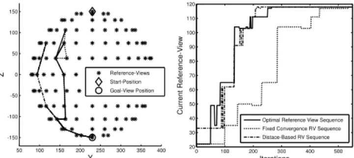
A virtual-reality simulation of a free moving camera allows the verification of the large view visual servoing scheme without being constrained by the robot kinematics or workspace. The camera navigates in 6 DOF around a sphere textured with a schematic map of the globe. The reference views are equidistantly located along longitudes and latitudes. The task is to guide the camera visually from the north to the south pole. Fig. 5 depicts the distribution of
0 100 200 300 400 500
20 30 40 50 60 70 80 90 100 110 120
Iterations
C u rr e n t R e fe re n c e -V ie w
50 100 150 200 250 300 350 400
-150 -100 -50 0 50 100 150
Y
Z
Optimal Reference View Sequence Fixed Convergence RV Sequence Distace-Based RV Sequence Reference-Views
Start-Position Goal-View Position
Fig. 5. Alignment of reference-views an comparison of chosen sequences from pole to pole on a sphere
reference-views together with the path pursued by the three methods under comparison. Even though the camera is initi- ally located above the north pole, all schemes immediately transit to an initial reference view that is already closer to the goal. The distance based method picks a different great circle route than the other two schemes as it ignores the issue of feature quality. A better rationale is to select the great circle route which guarantees perceptibility of a sufficient number of features for stable traverse to the south pole.
We term this effect the Pacific-problem, as for our globe
example, the equal-distant path either moving over America
or Africa contains more features due to the texture and
text on the continents than crossing the Pacific with sparse
features. The right part of fig. 5 compares the sequence
0 100 200 300 400 500 600 -200
-100 0 100 200 300 400 500
Iterations
Position
x [mm]
y [mm]
z [mm]
x [mm]
y [mm]
z [mm]
x [mm]
y [mm]
z [mm]
Distance-Based RV sel.
Fixed Convergence RV sel.
Optimal Reference View sel.
0 100 200 300 400 500 600
-200 -150 -100 -50 0 50 100 150 200 250 300
Iterations
Orientation
D [°]
E [°]
J [°]
D [°]
E [°]
J [°]
D [°]
E [°]
J [°]
Distance-Based RV sel.
Fixed Convergence RV sel.
Optimal Reference View sel.
Fig. 6. Pole to pole trajectories of the compared methods
and progression of reference views followed by the three alternative methods. Fig. 6 shows the evolution of the task space error in terms of translation and rotation. The number of iterations until convergence is approximately the same for the optimal image-based and the distance based navigation method. For the former the goal pose is reached within 300 iterations, for the later in about 290 iterations, whereas the static scheme with complete convergence takes about 560 iterations.
B. Navigation across a semi cylinder
The scheme is also evaluated in an experiment on a 5DOF Katana robot with an eye-in-hand camera configuration.
As the workspace of the manipulator is rather limited, the camera navigates across the inner surface of a semi cylinder with a circumference of 1.8m and a height of 0.4m. The inside of the semi cylinder is textured with a panoramic photo of our campus shown in fig. 7. This cylindric configuration is optimal with respect to the workspace of the robot as it allows a maximal number of sufficiently distinct reference views. The reference views form a 15 × 6 grid, horizontally separated by 10 °, vertically by 5cm. The kinematics of the specific robot limit the camera motion to 5 DOF. At the start pose the camera points at the upper left part of the image and the goal is located in the lower right corner of the cylinder.
As shown in Fig. 8, all methods follow at large a similar view-sequence. The only significant deviation occurs halfway through the path in a region which mostly contains sky and
Fig. 7. Experimental setup for visual servoing in 5 DOF on a semi cylinder
ground and therefore few distinctive features. The optimal switching scheme takes a small vertical detour in order to exploit the higher concentration of features in the textured band between sky and ground. The number of iterations
0 100 200 300 400 500 600
10 20 30 40 50 60 70
Iterations
R e fe re n c e -V ie w
0 500
-100 0 -50 50 150 100 200 -500 -400 -300 -200 -100 0 100 200 300 400 500
Y X
Z
Optimal Reference View Seq.
Fixed Convergence RV Seq.
Distance-Based RV Seq.
Reference-Views Start-Position Goal-View Position
Fig. 8. Alignment of reference-views and the chosen sequences
until final convergence is about 300 for the optimal method,
400 for the distance-based approach and 600 for the fixed-
convergence-method. The difference in time to convergence
results from the fact, that the two other methods require a
much longer time to traverse the region of sparse features
as the visual control tends to become unstable due to the
poorer quality of feature distributions. This observation is
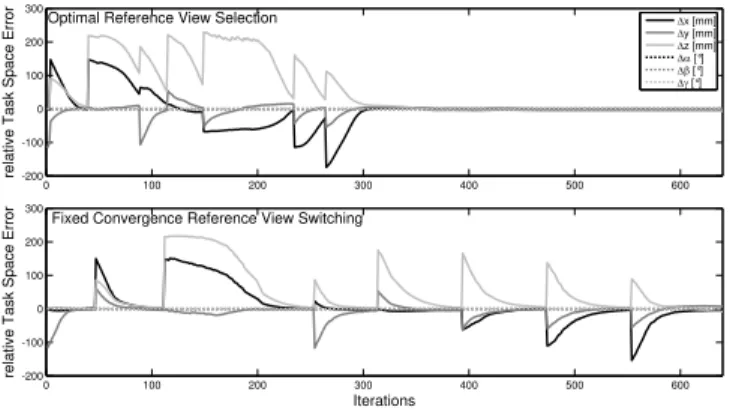
confirmed by an analysis of the evolution of the relative task
space error with respect to the intermediate reference views
shown in fig. 9. The upper graph depicts the progression of
task space error and switching sequence for the proposed
scheme the lower graph for the static scheme. The static
scheme wastes iterations in phases at which the feature error
is already low but not yet fully converged. The optimal cost
based scheme avoids delayed transition to the next reference
view, as it already switches for substantially larger residual
errors without compromising the stability of the control. The
sample rate of the visual control loop is approximately 4
Hz, limited the computational effort for feature extraction
(160 ms), online path planning and matching (70 ms) and
computation of visual features and differential kinematics (30
ms). The time for feature extraction is proportional to the size
0 100 200 300 400 500 600 -200
-100 0 100 200 300
re la ti v e T a s k S p a c e E rr o r
Optimal Reference View Selection
0 100 200 300 400 500 600
-200 -100 0 100 200 300
Iterations
re la ti v e T a s k S p a c e E rr o r
Fixed Convergence Reference View Switching
'x [mm]
'y [mm]
'z [mm]
'D [°]
'E [°]
'J [°]