U N I V E R S I T Y OF D O R T M U N D
R E I H E C O M P U T A T I O N A L I N T E L L I G E N C E COLLABORATIVE RESEARCH CENTER 531
Design and Management of Complex Technical Processes and Systems by means of Computational Intelligence Methods
Weighted moments of SIFT-features for decoupled visual servoing in 6DOF
Thomas Nierobisch, Johannes Krettek, Umar Kahn and Frank Hoffmann
No. CI-226/07
Technical Report ISSN 1433-3325 February 2007
Secretary of the SFB 531 · University of Dortmund · Dept. of Computer Science/LS 2 44221 Dortmund · Germany
This work is a product of the Collaborative Research Center 531, “Computational
Intelligence,” at the University of Dortmund and was printed with financial support of
the Deutsche Forschungsgemeinschaft.
Weighted moments of SIFT-features for decoupled visual servoing in 6DOF
T. Nierobisch, J. Krettek, U. Khan and F. Hoffmann
Chair for Control and Systems Engineering, University of Dortmund, Germany thomas.nierobisch@uni-dortmund.de
Abstract – Mobile manipulation in service robotic ap- plications requires the alignment of the end-effector with recognized objects of unknown pose. Image based visual servoing provides a means of model-free manipulation of objects solely relying on 2D image information. This con- tribution proposes a visual servoing scheme that utilizes the pixel coordinates, scale and orientation of the Scale Invari- ant Feature Transform (SIFT). The control is based on dy- namic weighted moments aggregated from a mutable set of redundant SIFT feature correspondences between the cur- rent and the reference view. The key idea of our approach is to weight the point features in a way that eliminates or at least minimizes the undesired couplings to establish a one- to-one correspondence between feature and camera motion.
The scheme achieves a complete decoupling in 4DOF, addi- tionally the visual features in 6DOF are largely decoupled except for some minor residual coupling between the hor- izontal translation and the two rotational degrees of free- dom. The decoupling results in a visual control in which the convergence in image and task space along a particular degree of motion is not effected by the remaining feature er- rors. Several simulations in virtual reality and experiments on a robotic arm equipped with a monocular eye-in-hand camera demonstrate that the approach is robust, efficient and reliable for 4DOF as well as 6DOF positioning.
Keywords: image based visual servoing, SIFT features, robotic manipulation, decoupled visual features
1 Introduction
This paper advocates SIFT features [1] for 6DOF visual servoing of a robotic manipulator with an eye-in-hand cam- era configuration. The increasing availability of inexpen- sive cameras and powerful computers opens a novel avenue for integrating image processing systems as a sensor for real-time control of robotic manipulators. Image and po- sition based visual servoing grows in visibility due to its importance for robotic manipulation and grasping [2].
Our point of departure is the conventional visual servoing paradigm developed for an eye-in-hand vision guided ma- nipulation task originally introduced in [3]. The visual point features are defined directly in the 2D image plane, there- fore a geometric object model or an explicit reconstruction
of the object pose becomes obsolete. The motion of a fea- ture with image coordinates f = (u, v) T is related to the camera motion via the image Jacobian or sensitivity matrix J v according to f ˙ = J v (r) ˙ r. Image based visual servoing builds upon this relationship by an error proportional con- trol law in which the error between reference features f ˆ and current features f is compensated by a camera motion
˙
r = −K · J v + (r)( ˆ f − f ), (1) in which J v + denotes the pseudo-inverse of the image Jaco- bian and K is a gain matrix. The computation of the analyt- ical image Jacobian requires knowledge about the depth of the scene and the intrinsic camera parameters. Image based visual servoing with point features suffers from the handi- cap that exclusive control of features in the image might re- sult in an inferior or infeasible camera motion. The underly- ing problem is caused by the coupling between translational and rotational degrees of freedom and is particularly immi- nent in the presence of substantial errors in orientation. In order to obtain a better motion control, the approach pro- posed in [4] decouples the translational and rotational de- grees of freedom by using the homography or the epipolar constraint held between the reference and the current im- age. In [5] the authors pursue a similar approach called 2-1/2 D visual servoing that includes a partial pose esti- mate to compensate the camera rotation. Both approaches require the online estimation of the homography or funda- mental matrix in the servo loop, with at least four or eight feature point correspondences. The scheme is fairly sensi- tive to image noise for poses close to the reference view.
The approach in [6] relies on image moments rather than points features to overcome the above mentioned shortcom- ings of visual servoing schemes. Our approach takes on the idea to design visual moments that are primarily sen- sitive to a single degree of motion and appear invariant to the remaining translations or rotations. Our scheme ex- ploits certain invariance properties of geometric moments to decouple visual features across different degrees of mo- tion. SIFT features for visual servoing applications were first introduced by [7], in which the authors explicitly re- construct the object pose based on the epipolar geometry.
A novel image-based controller that augments conventional
point features by the additional attributes scale and keypoint
orientation of SIFT features is presented in [8]. The visual features scale and keypoint orientation turn out to be widely independent of translation and rotation along the other axes which qualifies them to control the distance to the object and the rotation around the optical axis. Six generic vi- sual moments are defined based on the pixel coordinates, scale and orientation of multiple SIFT features. These mo- ments are dynamically adapted to the current geometric dis- tribution of available SIFT features. The trade-off between computational complexity and positioning accuracy is con- trolled by the number of scales at which SIFT-features are extracted. This contribution improves the moment based controller from [8] by completely decoupling the sensitiv- ity matrix for 4DOF based on a geometric constraint. Intro- ducing additional constraints, leads to a sensitivity matrix for visual servoing in 6DOF with only four off-diagonal el- ements, that exhibits a robust and efficient visual control of the robot pose.
The paper is organized as follows: Section 2 provides a brief description of the characteristics of SIFT-features, fol- lowed by the definition of the set of visual features for vi- sual servoing in 6DOF. Section 3 introduces the concept of a virtual centroid computed from weighted point features that eliminates the undesired couplings between the visual fea- tures and the degrees of freedom in 4DOF. In Section 4 the concept of weighted moments is extended to further decou- ple the sensitivity matrix for visual servoing in 6DOF. Sec- tion 5 compares the coupled and decoupled control scheme in 4DOF and 6DOF and analyzes their convergence prop- erties in robotic experiments. The paper concludes with a summary and outlook on future work in section 6.
2 Moments of SIFT-Features
Scale invariant feature transformations (SIFT) introduced by Lowe [1] occur frequently in textured objects and remain identifiable and distinguishable despite changes in scale, orientation, illumination and affine transformation. Each feature contains a compact representation of the surround- ing image region, the so called keypoint descriptor, which uniqueness distinguishes it from other features. Since these features are visible and robustly related across different views they are particularly suited for model free image based visual servoing. Once the image of the object is ac- quired from the demonstrated reference pose, the SIFT fea- tures are extracted automatically. For a detailed description of the automatic feature selection the interested reader is referred to [8]. A single SIFT-feature F i contains four at- tributes, namely the pixel coordinates u i and v i , the canoni- cal orientation of the keypoint φ i and its scale σ i . In the fol- lowing, the desired appearance of SIFT-features in the ref- erence position is denoted by F ˆ i = ( ˆ u i , v ˆ i , φ ˆ i , σ ˆ i ) and the current SIFT-features are denoted by F i = (u i , v i , φ i , σ i ).
n denotes the number of SIFT features correspondences es- tablished between the current and reference view. Scale and keypoint orientation are ideal to control the distance to the object and the rotation around the optical axis as they prove
widely insensitive to translation and rotation along the other axes [8]. A camera rotation around its optical axis by γ induces an inverse rotation of equal magnitude of the key- point orientations φ i . The averaged keypoint rotation f γ
regulates the camera rotation, whereas the translation along the camera axis is governed by visual feature f z defined as the average scale.
f γ = P n
i=1 φ i
n , f z = P n
i=1 σ i
n (2)
The point features u i , v i are first of all aligned with the camera orientation in the reference view according to the observed feature f γ . The correction along γ is therefore de- fined as ∆f γ = ˆ f γ − f γ . The visual features are rotated by ∆f γ such that the current SIFT feature locations u i and v i are aligned with the camera orientation in the reference view. The new SIFT feature locations u ′ i and v ′ i are deter- mined as follows,
u ′ i v ′ i
=
cos(∆f γ ) − sin(∆f γ ) sin(∆f γ ) cos(∆f γ )
· u i
v i
. (3) In the following the corrected pixel coordinates u ′ i and v ′ i are used for the computation of the remaining visual mo- ments and for better comprehensibility are denoted as u i
and v i . The moment based controller in [8] operates with the geometric centroid of point features for regulating trans- lations along the x- and y-axis. However, the geometric centroid suffers from a sensitivity to motions along the re- maining degrees of freedom. The visual features f x and f y
capturing translations along the x- and y-axis, are expressed as the weighted aggregation of the matched SIFT feature lo- cations
f x =
n
X
i=1
w i u i , f y =
n
X
i=1
w i v i (4) By proper selection of the weights w i attributed to individ- ual point features (u i , v i ) it is possible to decouple f x , f y from the remaining degrees of freedom. In order to com- plete the 6DOF visual control two additional visual features corresponding to the rotations about the x- and y- axis f α
and f β are defined. The visual features f α and f β capture the perspective distortions of lines connecting pairs of SIFT features caused by rotations.
f α =
n
X
i=1 n
X
j=i+1
(−ˆ v i − v ˆ j ) · k~ p j − ~ p i k P n
k=1
P n
l=k+1 k~ p k − ~ p l k (5) f β =
n
X
i=1 n
X
j=i+1
(−ˆ u i − u ˆ j ) · k~ p j − ~ p i k P n
k=1
P n
l=k+1 k~ p k − ~ p l k (6) The term k~ p j − p ~ i k denotes the length of the line connect- ing the two pixels, which weighted by the factor (−ˆ v i −ˆ v j ).
Its sign indicates whether the line is above or below the u-
scan-line through the cameras principal point. The absolute
magnitude of the weight increases with the vertical distance
from the image center. The visual feature f β represents the equivalent effect of dilations and compressions of lines caused by rotations along the y-axis. In the following the image Jacobian is derived in order to analyze the remaining couplings. The centroid feature [f x , f y ] T behaves similar to a virtual point feature and the Jacobian is obtained by aver- aging the individual point feature Jacobians stated in [2]
J f
x,f
y= P n
i =1
"
λ
z 0 −u z
i−u λ
iv
iλ
2+u λ
2i0 λ z − z v
i−λ
2λ −v
2iu
iz · v
i#
n (7)
in which λ denotes the focal length and z denotes the dis- tance between the camera and the feature plane. The main difference with respect to a point feature is the simplifying assumption that all SIFT-features share the same depth z.
This assumption is reasonable as long as the depth of the scene is small compared to the distance to the camera. The image Jacobian for the visual feature f α is given by
J f
α= P n
i=1, j=i+1
p
ij√ · ˆ v
ij·λ 8 · z
20 0 − 2 ·λ z −v ij +u ij
P n
k=1
P n
l=i+1 k~ p k − ~ p l k
(8) in which v ij = (v i −v j )/2, u ij = (u i −u j )/2 , v ˆ ij = (ˆ v i + ˆ
v j )/2, u ˆ ij = (ˆ u i +ˆ u j )/2 and the length p ij = kp i − p j k. In the Jacobian for the analogous visual feature f β the u and v components are interchanged. The resulting full 6DOF Jacobian matrix exhibits the following block structure.
f ˙ x
f ˙ y
f ˙ z
f ˙ α
f ˙ β f ˙ γ
=
K x 0 K ˜ xz K ˜ xα K ˜ xβ 0 0 K y K ˜ yz K ˜ yα K ˜ yβ 0
0 0 K z 0 0 0
0 0 0 K α K ˜ αβ 0 0 0 0 K ˜ βα K β 0
0 0 0 0 0 K γ
· T x
T y
T z
ω α
ω β
ω γ
(9) The objective of the remainder of this paper is to de- fine the dynamic weights w i in equation 4 in such a way that the residual couplings in the off-diagonal elements K ˜ xz , K ˜ xα , K ˜ xβ , K ˜ yz , K ˜ yα , K ˜ yβ disappear.
3 Decoupled visual servoing in 4DOF
With this objective in mind the features f x and f y are supposed to only depend on T x and T y , respectively. The following analysis for the proper dynamic weight focuses on the element K ˜ xz related to the u-component. Notice, that for the decoupling of the visual feature f y the same methodology is applied only using the v i instead of the u i . The undesired off-diagonal elements of the sensitivity ma- trix K ˜ xz is eliminated if the dynamic weights w i satisfy the constraint
K ˜ xz = J { f
x,z } =
n
X
i=1
w i
−u i
z = 0 (10) For an arbitrary set of point features (u i , v i ), this constraint is violated for the geometric centroid calculation with equal
weights w i = 1/n. In order to maintain the similarity with the conventional centroid we seek a minimal variation ∆w i
of the original weights w i = 1/n + ∆w i that satisfies the constraint. This optimal variation is obtained by minimiz- ing the following cost function in conjunction with a La- grange multiplier λ 1 .
F = 1/2
n
X
i=1
(w i − 1 n ) 2 + λ 1
n
X
i=1
w i u i (11) In order to solve the optimization problem the partial deriv- ative of 10 with respect to w i and the Lagrange multiplier λ 1 , not to be confused with the focal length λ, is computed as
∂F
∂w i
=
w u i − 1 n
+ λ 1 · u i = 0
∂F
∂λ 1
=
n
X
i=1
w u i · u i = 0
which in turn yields the least squares solution w i = 1
n − u i u ¯ P n
i=1 u 2 i , u ¯ =
n
X
i=1
u i
n (12)
Intuitively, the weight of SIFT features which pixels pos- sesses the opposite sign as the geometric centroid u ¯ = P
i u i /n is increased, whereas those with the same sign are down-weighted. Notice, that by definition the weighted centroid is always located at the origin of the current im- age thus f x = f y = 0. However, the reference features f ˆ x = P
i w i u ˆ i and f ˆ y = P
i w i v ˆ i are no longer constant, but depend indirectly on the current image via the dynamic weights w i and are therefore implicitly susceptible to mo- tions along multiple degrees of freedom. In order to verify the decoupling of the weighted visual features f x and f y
from a motion T z , it is necessary to show that the weights for an identical set of feature points remain indeed indepen- dent of the distance z. The following considerations assume that the image plane is oriented parallel to the feature plane.
The perspective projection of a world point on the image plane is given by u i = x i · f z , whereas the same point dis- placed by ∆z is projected to u i,∆z = x i · z+∆z f . Assum- ing that the weights w i fulfill the constraint
n
P
i=1
u i · w i , the weighted sum of the feature points u ′ i at distance z + ∆z is thus given by:
n
X
i=1
u i,∆z · w i = z z + ∆z ·
n
X
i=1
u i · w i = 0. (13)
Due to fact that z+∆z z is a proportional factor common to
all features, the optimal weights for the first set of feature
points also transform the virtual centroid of the second set
of feature points to zero. Nonetheless, the weights are effec-
tively down-scaled by the factor z+∆z z . In order to render
the weights themselves and not only the centroid indepen- dent of the distance z, the weights are normalized according to
w i,norm = w i ·
n
P
k=1
|w k |
n (14)
Under the assumption, that the weighted sum of the features points is initially zero for the reference view, the weights w i,norm transform the virtual centroid of every other view to the image center independent of the distance z. Figure 1 depicts two projections of the same features, in which the corresponding view points differ by a displacement ∆z.
The weights w i are optimized according to the first set of feature points, but are also applied to weight the second set. Both virtual centroids are located in the image center even though the weighted feature points for the two sets dif- fer. The example demonstrates that neither the weights nor the visual features f x and f y change with a camera motion along z. Notice, that in the weighted scheme the role of cur- rent and reference features are reversed. Typically, the ref- erence features are constant and the current features change with the motion of the camera. However, in the weighted scheme the current centroid (f x = 0, f y = 0) is constant per definition and always coincides with the principal point due to equation 10. Instead the reference features features f ˆ x , f ˆ y change over time as the weights w i change with the current view, even though the point features u ˆ i , v ˆ i them- selves are constant.
−2000 −1500 −1000 −500 0 500 1000 1500 2000
−300
−200
−100 0 100 200 300 400
u
v
Features 2 Features 1
Features 1 weighted Features 2 weighted
Figure 1: Virtual centroid for two sets of feature points at different distances between camera and feature plane
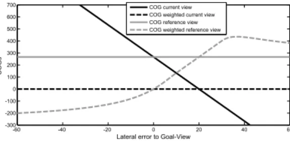
Figure 2 depicts the image projections of the conven- tional and weighted centroid u-components view as a func- tion of the lateral task space error ∆x. The two hori- zontal lines correspond to the constant conventional refer- ence centroid and the constant weighted current centroid u- components. In this example, the reference image is delib- erately chosen such that the majority of features is located in the right half plane. Therefore, the conventional cen- troid is shifted along the u-component by 120 units from the principal point. The current conventional centroid de- pends linearly on the lateral error and intersects the refer- ence centroid for a zero lateral error ∆x = 0. However, the offset and slope depend on the longitudinal distance be-
tween camera and feature plane. Current and reference fea- tures interchange their role for the weighted scheme, in that the former remains constant and the later changes with the lateral error in a nonlinear fashion. In this case the depen- dency of the centroid on the lateral error remains the same independent of the longitudinal pose error in z. Again, the reference and current centroid intersect for zero lateral er- ror. Even though the slopes for the weighted and conven- tional centroid exhibit opposite sign, the actual image error f ˆ x − f x has the same sign for both schemes. The figure also reveals the slight asymmetry of the weighted reference centroid for positive and negative lateral errors. For large positive lateral errors the image error even increases slightly with decreasing lateral error. This asymmetry is caused by the inhomogeneous distribution of point features u i , which in turn effects the adaptation of the weight factors through equation 12. It should be noted, that the asymmetry and slope inversion do not effect the stability or convergence of the visual control and only occur if the point feature distri- bution in the reference image is significantly skewed.
-60 -40 -20 0 20 40 60
-300 -200 -100 0 100 200 300 400 500 600 700
Lateral error to Goal-View
COGs
COG current view COG weighted current view COG reference view COG weighted reference view
Figure 2: Centroid u-component as a function of the lat- eral error for the conventional and weighted centroid in the current and reference view
4 Decoupled visual servoing in 6DOF
Section 3 discussed a fully decoupled sensitivity matrix for visual servoing in 4DOF. This section is aimed at ex- tending the decoupling to visual servoing in 6DOF. This requires that the features f x and f y do not only become in- dependent on the motion T z but also on the rotary motions ω α and ω β . Again, the constraints emerge from an analy- sis of the Jacobian in equation 7. The optimization problem for decoupling the visual feature f x from the motions T z
and ω α according to the Jacobian in equation 5 is stated as follows:
F = 1 2
n
X
i=1
w i − 1
n 2
+ λ 1 ·
n
X
i=1
w i · u i (15)
+ λ 2 ·
n
X
i =1
w i · u i · v i
Theoretically, it would be possible to cancel the compo- nent
n
P
i=1
w i · λ 2 + u 2 i
of the Jacobian related to the mo-
tion ω β as well. If this additional constraint is included,
the minimization problem in equation 15 is algebraically still solvable. Unfortunately, the inclusion of this constraint substantially reduces the sensitivity of the feature f x to its associated motion T x , resulting in a deterioration of the vi- sual control. Therefore, the weight optimization problem only includes constraints for the cancellation of the ele- ments K ˜ xα and K ˜ yβ in the sensitivity matrix in equation 9.
The cost function F is partially differentiated with respect to w i and the Lagrangian multipliers λ i .
∂F
∂w i
= w i − 1
n + λ 1 · u i + λ 2 · u i · v i
∂F
∂λ 1
=
n
X
i=1
w i · u i
∂F
∂λ 2
=
n
X
i=1
w i · u i · v i
Changing to vector notation by substituting k = ( 1 n , . . . , n 1 ) u = (u 1 , . . . , u n ) and p = (u 1 · v 1 , . . . , (u n · v n ) a set of linear equations is obtained: w + λ 1 u + λ 2 p = k, with the constraints w · u = 0, w · p = 0. In order to determine the Lagrangian multipliers, the weights w are eliminated by multiplying with the transpose of u and s. This results in a system of linear equations, which can be solved in closed from.
u T u u T p p T u p T p
· λ 1
λ 2
= u T k
p T k
(16) The corresponding weights of the point features are deter- mined as follows w = k − λ 1 ·u − λ 2 ·p and subsequently normalized according to equation 14. However, some resid- ual coupling remains through the non-zero off-diagonal ele- ments ( K ˜ xβ , K ˜ yα , K ˜ αβ , K ˜ βα ) in the Jacobian. These terms capture the effect of a rotation α along the x-axis on the mo- tion of the v-components of point features, and vice versa a rotation β along the y-axis on the u-component.
5 Experimental results
The proposed scheme is evaluated for a free moving camera in virtual reality and in experiments on a 5DOF KATANA manipulator with an eye-in-hand configuration.
This section reports results for the 4DOF case on the manip- ulator and the 6DOF case in virtual reality as the KATANA robot is restricted to 5DOF. For the evaluation of the de- coupled visual features for 4DOF visual servoing, the ma- nipulator is dislocated from the reference pose by an initial displacement ∆x = 20mm, ∆z = 40mm and ∆γ = 25°.
Substantially larger displacements are not feasible in the ex- periments due to the restricted workspace of the KATANA manipulator and the eye-in-hand constraint of keeping the object in view of the camera. Figure 3 compares the evolu- tion of the task space error and the image error for the orig- inal coupled controller (left) and the decoupled controller (right). In case of the coupled controller the z-error intro- duces a dynamic shift of the current feature f x . Although the image space error itself is compensated after 12 itera- tions the corresponding residual task space error in x re- mains until complete cancellation of the ∆z after about 25
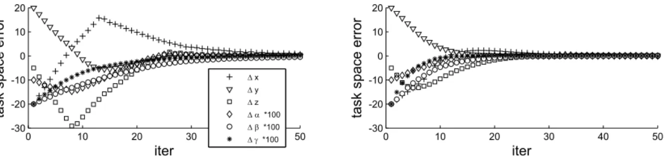
iterations. The decoupled controller eliminates the impact of T z on feature f x such that image and task space error in the x-component disappear simultaneously after 12 itera- tions. Even though there is no initial displacement along the y-axis, the inherent coupling with T z induces an undesired motion in task space ∆y ≈ 5mm. Again, the decoupled controller eliminates this detrimental disturbance and ∆y is not effected by the motions T x or T z . The residual task space error of the decoupled controller is less than 0.5mm for the position and 0.5° for the rotation. Figure 4 shows the task space error for visual servoing for 6DOG in a virtual reality simulation. Notice, the substantial coupling among the different degrees of freedom in the task space for the conventional controller (left). The translational motions in x, y and z demonstrate a significant overshoot caused by the couplings of the conventional centroids f x , f y with T z , ω α and ω β . The task space errors in x and z initially in- crease and only start to converge after stabilization of the other errors. For the weighted centroid control (right) with the partially decoupled Jacobian the disturbances are signif- icantly reduced and the six pose errors converge smoothly and largely independent of each other. The residual over- shoot in the x and y components is caused by the remaining coupling with ω β and ω α , respectively. The results clearly demonstrate that the weighted features result in a more fa- vorable task space motion of the camera.
6 Conclusions and Future Work
This contribution presented a novel approach for visual servoing based on decoupled moments of SIFT-Features.
The properties of SIFT-features render the approach univer- sally applicable for manipulation of daily-life objects that exhibit some texture. SIFT-features for visual servoing ap- plications offers the further advantage that object recogni- tion and pose alignment of the manipulator rely on the same representation of the object. For 4DOF visual servoing a set of completely decoupled visual features is introduced, that results in robust and independent convergence of the corre- sponding task space errors. Problems of the classical Jaco- bian based visual servoing scheme like the camera retreat problem and local minima are resolved. A novel sensitiv- ity matrix for 6DOF visual servoing is introduced, which has only four off-diagonal couplings between the visual fea- tures and the degree of motion. The visual control with the novel causes the pose errors to converge largely indepen- dent of each other resulting in a smoother task space mo- tion of the camera. In future work we intend to accomplish large view visual servoing. Due to the limited visibility and perceptibility of SIFT-features across different views, it be- comes necessary to introduce additional intermediate refer- ence views to navigate across the entire view hemisphere.
Future research is dedicated to identify intermediate views
and to define an appropriate cost function that governs the
transition between overlapping reference views in a stable,
robust and time-optimal manner.
0 10 20 30 40 50 -20
-10 0 10 20 30 40
iter
im a g e s p a c e e rr o r
0 10 20 30 40 50
-20 -10 0 10 20 30 40
iter
im a g e s p a c e e rr o r ' f
x
' f
y' f
z' f
J0 10 20 30 40 50
-40 -30 -20 -10 0 10 20
iter
ta s k s p a c e e rr o r
0 10 20 30 40 50
-40 -30 -20 -10 0 10 20
iter
ta s k s p a c e e rr o r
' x [mm]
' y [mm]
' z [mm]
' J [°]
Figure 3: Left top & bottom) Image and task space error for visual servoing in 4DOF, Right top & bottom) Image and task space error for decoupled visual servoing in 4DOF
0 10 20 30 40 50
-30 -20 -10 0 10 20
iter
ta s k s p a c e e rr o r
0 10 20 30 40 50
-30 -20 -10 0 10 20
iter
ta s k s p a c e e rr o r
' x ' y ' z ' D *100 ' E *100 ' J *100