Visual servoing with moments of SIFT features

U N I V E R S I T ¨ A T D O R T M U N D

REIHE COMPUTATIONAL INTELLIGENCE S O N D E R F O R S C H U N G S B E R E I C H 5 3 1

Design und Management komplexer technischer Prozesse und Systeme mit Methoden der Computational Intelligence

Visual Servoing with Moments of SIFT Features

Frank Hoffmann, Thomas Nierobisch, Thorsten Seyffarth and G¨ unter Rudolph

Nr. CI-207/06

Interner Bericht ISSN 1433-3325 May 2006

Sekretariat des SFB 531 · Universit¨ at Dortmund · Fachbereich Informatik/XI 44221 Dortmund · Germany

Diese Arbeit ist im Sonderforschungsbereich 531,

” Computational Intelligence“, der

Universit¨ at Dortmund entstanden und wurde auf seine Veranlassung unter Verwendung

der ihm von der Deutschen Forschungsgemeinschaft zur Verf¨ ugung gestellten Mittel

gedruckt.

Visual Servoing with Moments of SIFT Features

Frank Hoffmann, Thomas Nierobisch ^∗ , Torsten Seyffarth ^∗ and G¨unter Rudolph ^†

∗ Chair for Control System Engineering/Electrical Engineering and Information Technology/University of Dortmund, Germany {frank.hoffmann, thomas.nierobisch, torsten.seyffarth}@uni-dortmund.de

† Chair of systems analysis/Department of Computer Science/University of Dortmund, Germany guenter.rudolph@cs.uni-dortmund.de

Abstract— Robotic manipulation of daily-life objects is an essential requirement in service robotic applications. In that context image based visual servoing is a means to position the end-effector in order to manipulate objects of unknown pose.

This contribution proposes a 6 DOF visual servoing scheme that relies on the pixel coordinates, scale and orientation of SIFT features. The control is based on geometric moments computed over an alterable set of redundant SIFT feature correspondences between the current and the reference view.

The method is generic as it does not depend on a geometric object model but automatically extracts SIFT features from images of the object. The foundation of visual servoing on generic SIFT features renders the method robust with respect to loss of redundant features caused by occlusion or changes in view point.

The moment based representation establishes an approximate one-to-one relationship between visual features and degrees of motion. This property is exploited in the design of a decoupled controller that demonstrates superior performance in terms of convergence and robustness compared with an inverse image Jacobian controller. Several experiments with a robotic arm equipped with a monocular eye-in-hand camera demonstrate that the approach is efficient and reliable.

I. INTRODUCTION

This paper advocates SIFT features for 6-DOF visual ser- voing of a robotic manipulator with an eye-in-hand cam- era configuration. The increasing availability of inexpensive cameras and powerful computers opens a novel avenue for integrating image processing systems as a sensor for real- time control of robotic manipulators. Image and position based visual servoing grows in visibility due to its importance for robotic manipulation and grasping [1].

Our point of departure is the conventional visual servoing paradigm developed for an eye-in-hand vision guided ma- nipulation task originally introduced in [2]. The visual point features are defined directly in the 2D image plane, therefore a geometric object model or an explicit reconstruction of the object pose becomes obsolete. The motion of a feature with image coordinates f = (u, v) ^T is related to the camera motion via the image Jacobian or sensitivity matrix J v according to

f ˙ = J v (r) ˙ r. (1) Image based visual servoing builds upon this relationship by an error proportional control law in which the feature error f ˆ − f is compensated by a camera motion

˙

r = −K · J _v ⁺ (r)( ˆ f − f ), (2)

in which J _v ⁺ denotes the pseudo-inverse of the image Jacobian and K is a gain matrix. The computation of the analytical image Jacobian requires knowledge about the depth of the scene and the intrinsic camera parameters.

Image based visual servoing with point features suffers from the handicap that exclusive control of features in the image might result in an inferior or infeasible camera motion. The underlying problem is caused by the coupling between trans- lational and rotational degrees of freedom and is particular imminent in the presence of substantial errors in orientation.

As a remedy to these shortcomings [3] proposes a visual servoing scheme based on image moments rather than point features. Low-order moments represent geometric properties of projected objects such as areas, centroids or principal axes.

Moments describe generic geometric entities that do not refer to a specific object shape or appearance. They are easily com- puted from a segmented image or as in our case from a discrete set of distinguishable feature points. The key idea is to define visual moments in a way that renders them invariant under certain translations or rotations. These invariance properties are then exploited to decouple visual features across different degrees of motion. A substantial amount of research has been devoted to identify such invariant moments [4], [5], [6].

y z

D

E J

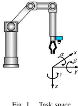
Fig. 1. Task space

Visual servoing with scale invariant feature transformation

(SIFT) [7] was first introduced by [8]. Their approach focuses

on the robust feature extraction and view point reconstruction

based on the epipolar geometry. Our contribution emphasizes

the design of a novel image-based controller that augments

conventional point features by the additional attributes scale

and keypoint orientation of SIFT features. The visual features

scale and keypoint orientation turn out to be widely indepen-

dent of translation and rotation along the other axes which

makes them suitable to control the distance to the object and the rotation around the optical axis. The pixel coordinates, scale and orientation of multiple SIFT features are aggregated into six generic visual moments for 6-DOF motion control.

The control scheme is robust as the visual features are based upon generic weighted moments which are computed over a variable subset of SIFT features. This property eliminates the need of complete matching between features in the reference and current image. Instead The visual moments are dynami- cally adapted to the current geometric distribution of available SIFT features. Using more SIFT features increases the ac- curacy of the control at the cost of increased computational complexity for extracting and matching them across different object views. This trade-off suggests an approach that initially employs only few SIFT features for coarse but fast control at large image errors and gradually incorporates additional features as the camera converges to the reference pose.

This paper compares two moment based controllers in terms of control design complexity and convergence of the control.

The first scheme explicitly calculates the image Jacobian for the moment based features at each control step. This method requires knowledge about the distance between camera and object in the reference pose in order to recover the depth of the scene. The second approach is computationally simpler as it neglects the undesired minor couplings between camera and feature motion. Instead each degree of freedom is controlled by a single visual feature, which separates the control design into six decoupled linear control laws.

The manipulator and camera configuration are shown in figure 1. In order to comply with the usual camera coordinate frame, the Z-axis is aligned with the optical axis, whereas the X-axis and the Y-axis of the manipulator span the horizontal plane. Rotations around the X-, Y-, Z-axis are denoted by α, β, γ. The corresponding velocities are denoted by T x , T y , T z and ω α , ω β , ω γ .

The paper is organized as follows: Section II provides a brief description of the SIFT algorithm. It also introduces the automatic feature identification with the objective to detect stable and unambiguous SIFT features that remain visible over a large region of the manipulator workspace. Section III describes the integration of additional attributes scale and keypoint orientation to complement the set of visual features.

It also explains how the primitive features are aggregated into moments that provide the basis for visual servoing. The derivation of the corresponding image Jacobian and the design of two different visual servo controller are the topic of section IV. Section V compares the two variants of the control scheme and analyzes their convergence behaviors in experiments with a 5-DOF robotic manipulator. The paper concludes with a summary and outlook on future work in section VI.

II. I DENTIFICATION OF ROBUST SIFT FEATURES

Scale invariant feature transformations (SIFT) introduced by Lowe [7] are identifiable irrespective of scale, orienta- tion, illumination and affine transformations. SIFT features occur frequently on textured objects and are discriminated by

their associated keypoint descriptor which contains a com- pact representation of the surrounding image region. These characteristics make them particular attractive for model free image based visual servoing, as the same features are visible and robustly related across different views. A set of SIFT features is automatically extracted from the image of the object captured in the demonstrated reference pose. The computa- tional complexity for extracting and matching SIFT features is feasible for real-time image based control. In the context of visual servoing SIFT features include the additional attributes scale and orientation which provide valuable information to regulate the depth and orientation around the camera axis.

The image based controller operates with statistical first and second order moments computed over a set of SIFT features matched between the current and the reference view. This approach is robust with respect to occlusion, illumination and perspective distortions as the performance and convergence of the controller is not jeopardized as long as some features in the current image still match with reference features. It is important to achieve reliable correspondences as a single incorrect reference feature might effect the proper convergence to the goal pose. Depending on the texture and the parameter settings of the SIFT algorithm a typical image of size 500×500 pixels contains up to hundreds of stable SIFT features [7].

Feature identification assumes the important role to identify optimal features in terms of discrimination, stability and detectability across the workspace. SIFT features in the current image are matched with their corresponding reference features by comparison of their distinctive keypoint descriptors.

Naturally, the keypoint descriptors of the same feature in different views are, although similar, not exactly identical. This variation might lead to incorrect associations between features if two actually different SIFT features share similar keypoint descriptors. The objective of the automatic feature selection is to establish reliable correspondences between different appear- ances of the same feature across different poses. Candidates for stable and unambiguous SIFT features are evaluated according to similarity, keypoint orientation and epipolar consistency. In a first analysis, those pairs of ambiguous SIFT features in the reference image which are too similar to each other are rejected to avoid later confusion between them.

In the second stage the remaining candidate SIFT features are extracted and matched across different views uniformly distributed over the entire workspace. The new correspon- dences are verified by means of the consistent keypoint rotation and the epipolar constraint. The keypoint criterion compares the relative keypoint orientations between matched features. A rotation around the camera axis causes an equiva- lent rotation of the keypoint descriptors. Matched feature pairs for which the change in keypoint orientation is not consistent with the overall rotation are eliminated from the database. The keypoint orientation criterion is applied online during control to continuously verify the consistency of matched feature pairs.

The epipolar constraint provides an additional criterion to

eliminate incorrectly matched SIFT features. For the verifi-

cation views the relative pose and orientation of the camera with respect to the reference pose are calculated based on the manipulator kinematics. In conjunction with the cameras intrinsic parameters this information is sufficient to estab- lish the epipolar geometry between the two views expressed through the essential matrix [9]. A feature in the current view is constrained to the epipolar line defined by the epipolar geometry and the location of the corresponding reference feature in the other image. If the orthogonal distance between the feature and its corresponding epipolar line exceeds a threshold the match is presumably incorrect and the feature is rejected. Depending on the texture of the object, the parameter settings of the SIFT algorithm and the distance to the object at the reference pose about 10-100 verified SIFT features succeed on all tests and are included in the database of reference features. The robustness of the feature selection is confirmed as false correspondences of the verified features did not occur during the experiments.

Figure 2 illustrates the set of extracted and verified features in the reference view. The dots represent the initial set of can- didate SIFT features. From this initial set, twenty-six features indicated by crosses exhibit sufficiently distinctive keypoint descriptors to pass the similarity test. The circles correspond to the final set of sixteen features in compliance with the epipolar constraint and the consistent keypoint criterion. SIFT feature extraction and matching runs at a rate of approximately 7Hz for a camera resolution of 320 × 240 pixels on a Pentium 4 running at 2.8 GHz.

Fig. 2. Extracted and verified SIFT-Features

III. G ENERIC VISUAL FEATURES

This section describes the generation of moment based visual features from the primitive attributes pixel coordinates, scale and orientation of SIFT-features. A single SIFT-feature F i contains four attributes, namely the pixel coordinates u i and v i , the canonical orientation of the keypoint φ i and its scale σ i . In the following, the desired appearance of SIFT-features in the reference position is denoted by F ˆ _i = ( ˆ u _i , v ˆ _i , φ ˆ _i , σ ˆ _i ) and the current SIFT-features are denoted by F i = (u i , v i , φ i , σ i ).

The rotation of the camera along the optical axis is recovered from the change in keypoint orientation f γ . The remaining visual features f x , f y , f z , f α and f β are computed after the

current image has been aligned with the reference image by a counterrotation according to f γ . The conventional image based visual servoing with point features suffers from the shortcoming that the coupling between translational and ro- tational components might result in singularities or infeasible camera trajectories [10],[11]. The approach in [10] is based on a cylindrical coordinate system in order to achieve a better decoupling of the T z and the ω γ component. The approach in [11] employs line features which orientation decouples the rotation ω γ from the translational components.

In our approach the rotation around the camera axis is regulated by the canonical orientation φ i of SIFT-features and is therefore decoupled from the translation. A rotation of the camera by γ causes an equivalent rotation of the keypoint orientations φ i by the same amount. The reference view is defined by the SIFT-features selected during the automatic feature extraction stage. A set of SIFT-features is extracted from the current view from which n matches with the reference features are established. The visual feature f γ is defined by the average keypoint orientation

f γ = P n

i =1 φ i

n . (3)

in which the φ i are represented by their sine and cosine in order to compute a proper angular mean. The feature error for the γ correction ∆f γ is defined as:

∆f γ = ˆ f γ − f γ (4) The original SIFT feature locations u i and v i are aligned with the camera orientation in the reference view by applying the inverse rotation by an amount of ∆f γ :

u ⁰ _i v _i ⁰

=

cos(∆f γ ) − sin(∆f γ ) sin(∆f γ ) cos(∆f γ )

· u i

v i

. (5) The corrected pixel coordinates u ⁰ _i and v _i ⁰ become independent of the camera rotation and form the basis for the computation of the remaining visual moments.

In the following we analyze the accuracy of the rotation es- timate and its robustness with respect to changes in viewpoints caused by camera rotations along the other axes. The camera is rotated around the optical axis over the entire range −π to π in discrete steps of ₆₄ ^π . The distribution of the error between the estimated mean computed over all SIFT-features and the true rotation is shown in Figure 3. The upper graph depicts the error estimate ε γ in degrees as a function of the rotation γ, with a reference orientation of 0°. The maximum error of about 1.3° occurs at a rotation of about 100°. The lower graph shows the distribution of the error ε γ across the 128 rotation steps.

The mean absolute error amounts to |ε γ | = 0.52° the standard deviation σ γ of the error distribution ε γ is about 0.4°. Notice, that the absolute error in the estimated orientation is smaller for rotations close to the reference orientation which eventually determines the residual orientation error for the visual control.

This accuracy in orientation is confirmed in the closed-loop

control visual servoing experiments.

−1.5 0 −1 −0.5 0 0.5 1 1.5 10

20

ε

frequency

−150 −100 −50 0 50 100 150

−1 0 1

γ ε

µ

σ

Fig. 3. Estimation error for γ across absolute orientations from π to −π

∆ α 0 5 10 15 20 25 30

|ε

| 0.52 0.26 0.36 1.05 0.88 0.92 1.13 σ 1.13 1.50 1.10 2.60 3.11 3.44 4.59

TABLE I

E

∆ α

.

The average SIFT-feature keypoint orientation coincides with the camera orientation, which guarantees a unique min- imum and the stability of visual control of γ by the feature

∆f _γ .

Even if the image and feature plane are not parallel the perspective distortion of the SIFT feature caused by a camera rotation along an orthogonal axis hardly hampers the rota- tion estimate ∆f γ which still accurately captures the camera orientation. Table I shows that orthogonal rotations along α only have a minor effect on the accuracy of ∆f _γ . Rotations of more than 30° cause affine deformations for which the SIFT keypoint descriptors in different views are no longer compliant. For rotations of up to 30° the mean absolute error increases to |ε γ | = 1.13° which is still accurate enough for the application at hand. The visual features for the remaining translational and rotational degrees of freedom are computed as geometric moments over the distribution of SIFT feature pixel coordinates u ⁰ _i and v _i ⁰ and average scale σ i . Visual features f x and f y are expressed by the centroid of matched SIFT features.

f x = P n

i =1 u ⁰ _i

n , f y = P n

i =1 v _i ⁰

n (6)

The centroid primarily captures the horizontal translation of the camera but also varies with motions in z, α and β. The vertical translation T z is coupled with the average distance between pairs of feature points

f zd = P n

i =1

P n j = i +1

q (u ⁰ _i − u ⁰ _j ) ² + (v ⁰ _i − v _j ⁰ ) ²

n

2 · (n − 1) (7)

that captures the average scale of the scene. Computing the scale from the distance between point features that f zd is

not invariant with respect to perspective distortions caused by rotations along the other two axes. Therefore, the feature f zd

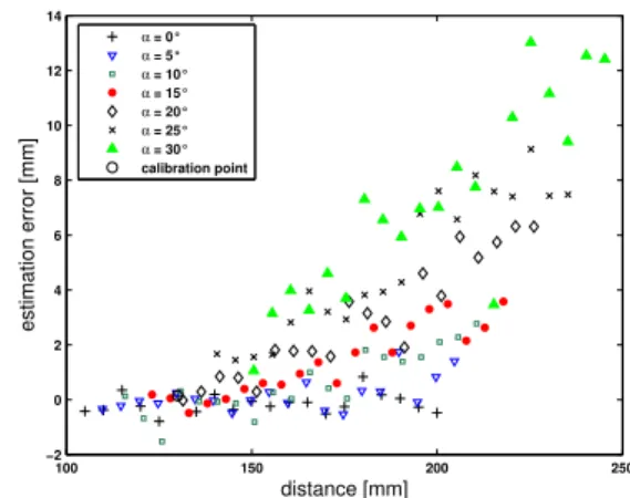
is replaced by the inherent scale of SIFT-features. Figure 4 depicts the variation of scale σ for typical SIFT-features as a function of the distance z between the object and the camera.

The scale of SIFT-features is given by ^K _z . The constant gain K depends on the focal length of the camera multiplied by the initial scale of the feature. The visual feature f z σ is defined

0.2 0.3 0.4 0.5 0.6 0.7

0 5 10 15 20 25 30

distance [m]

scale

SIFT−Feature 1 SIFT−Feature 2 SIFT−Feature 3 SIFT−Feature 4 SIFT−Feature 5 1/z

Fig. 4. Scale versus distance

as the average scale:

f zσ = P n

i =1 σ i

n (8)

Notice, that in principle a single SIFT feature is sufficient to compute f zσ . The actual distance z is recovered from the scales σ i under the assumption that the initial distance z ˆ at the reference image is known.

z = ˆ z P n

i =1 σ ˆ

σ

n (9)

The feature f zσ is largely decoupled from the other degrees of motion. Figure 5 shows the estimation error in z as a function of the absolute distance and the camera rotation α. Notice,

100 150 200 250

−2 0 2 4 6 8 10 12 14

distance [mm]

estimation error [mm]

α = 0°

α = 5°

α = 10°

α = 15°

α = 20°

α = 25°

α = 30°

calibration point

Fig. 5. Error in the z-estimate as a function of the distance and change in orientation α

that the reference scale is captured at a nominal distance

z = 130mm. The absolute error increases with distance

and tilt angle of the camera. Again, the feature error in the vicinity of the reference pose determines the residual task space error, which is less than 1mm at the correct pose. This level of accuracy is confirmed in the closed-loop control visual servoing experiments.

The 6-DOF visual control is completed by the visual features f α and f β that capture the rotations along the x- and y-axis. Both features represent the effect of perspective distortions on lines caused by the yaw and pitch motion of the camera. Figure 6 illustrates the effect for a square configuration of four feature points that form six lines. The left hand side depicts the image of the square for parallel feature and image plane, the right hand side the image with the camera is tilted around the x-axis and a compensation of the shift along the y-direction. The distortion increases the length of line 1 and simultaneously decreases the length of line 3. This dilation and compression of lines is captured by the feature

f _α = P n

i =1

P n

j = i +1 (−ˆ v i − ˆ v j ) · (k~ p j − ~ p i k − f zd )

n

2 · (n − 1) (10)

The term k~ p _j − ~ p _i k denotes the length of the line connecting the two pixels which is multiplied by the weight factor (−ˆ v i − ˆ

v j ). Its sign indicates whether the line is above or below the u-scan-line through the cameras principal point. The absolute magnitude of the weight increases with the vertical distance from the image center. The lines 2, 4, 5, 6 possess a weight factor of zero as v ˆ i and ˆ v j cancel each other. In case of the square the product of the weight factor and variation in length has the same sign for lines 1 and 3. The term f zd according to equation 7 captures the variation in pixel pair distances caused by changes in depth. Its subtraction partially compensates the effect of dilations caused by zooming in along the z-direction on f α . The visual feature

f β = P n

i =1

P n

j = i +1 (−ˆ u i − u ˆ j ) · (k~ p j − ~ p i k − f zd )

n

2 · (n − 1) (11)

represents the equivalent effect of dilations and compressions of lines caused by rotations along the y-axis. Notice, that

3

2 4

6 5

1

3 1

2 4

6 5

v

u

v

u

Fig. 6. Perspective distortion caused by camera tilt

for the configurations in 6 the feature f β remains constant although the length of vectors |~ p j − ~ p i k changes.

IV. C ONTROLLER D ESIGN

The visual control scheme refers to the image Jacobian for the set of visual features defined in the previous section.

In the following two different controllers are designed and analyzed. The first design is based on the exact inversion of the image Jacobian, whereas the second decoupled controller controls each degrees of motion by a single feature and ignores the remaining cross-couplings between feature and camera motion. Both controllers share an independent linear control of the rotation around the camera axis ∆γ based on the visual feature f γ . The exact controller employs the visual feature f zd , whereas the decoupled control scheme generates f zσ from the average scale of SIFT-features. The controllers map the error between the features in the goal and the current view

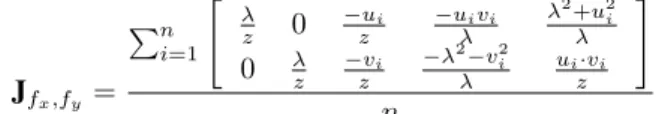
∆f = [ ˆ f x , f ˆ y , f ˆ z , f ˆ α , f ˆ β ] ^T − [f x , f y , f z , f α , f β ] ^T (12) to a camera motion in five degrees of freedom ∆r = [∆x, ∆y, ∆z, ∆α, ∆β ] ^T . The first control design utilizes equation 1 and requires the online calculation and inversion of the image Jacobian for the set of visual features. The centroid feature [f x , f y ] ^T behaves like a virtual point feature and the Jacobian is simply obtained by the averaging the individual point feature Jacobians stated in [1].

J f

,f

= P n

i =1

"

λ

z 0 ^−u _z

^−u _λ

^v

^λ

⁺ _λ ^u

0 ^λ _z ^−v _z

^−λ

_λ ^−v

^u

_z ^·v

#

n

The main difference with respect to a point feature is the simplifying assumption that all SIFT-features share the same depth, which is extracted from their scale by means of equation 9. This assumption is reasonable as long as the depth of the scene is small compared to distance to the camera.

The image Jacobian for the remaining visual features f _z , f _α , f _β becomes

J f

= P n

i=1, j=i+1

p ji ·

0 0 ¹ _z − ^v _λ

^u _λ

n

2 · (n − 1)

J f

= P n

i=1, j=i+1

p ij · h

0 0 − ^{2·ˆ v} _z

^{2·ˆ v}

_λ ^·v

− ^{2·ˆ v}

_λ ^·u

i

n

2 · (n − 1) +

P n

i=1, j=i+1

2 · ˆ v ij n

2 · (n − 1) · J f

J f

= P n

i=1, j=i+1

p ji · h

0 0 − ^{2·ˆ u} _z

^{2·ˆ u}

_λ ^·v

− ^{2·ˆ u}

_λ ^·u

i

n

2 · (n − 1) +

P n

i=1, j=i+1

2 · u ˆ ij n

2 · (n − 1) · J f

in which the center point of the feature pair (i, j) is defined by v _ij = (v _i + v _j )/2, u _ij = (u _i + u _j )/2 , v ˆ _ij = (ˆ v _i + ˆ v _j )/2, ˆ

u ij = (ˆ u i + ˆ u j )/2 and its length by p ij = kp i − p j k.

The camera motion results from the product of the feature error with the inverse of the image Jacobian and the diagonal gain matrix

∆r = −K · J _v ⁻¹ · ∆f (13)

The proportional gains in the matrix K are designed by means of linear controller design considering the time delay of the image processing and servoing loop. The visual features are specifically designed such that they are sensitive to one par- ticular degree of motion and relatively invariant with respect to the remaining motions. This property suggests a simplified controller design in which the off-diagonal elements of the Jacobian J v are neglected and the control assumes a one- to-one scalar relationship between features and degrees of motion. The sensitivity matrix

















 f ˙ x

f ˙ y

f ˙ z

f ˙ α

f ˙ β

f ˙ γ



















=

















K x 0 K ˜ xz K ˜ xα K ˜ xβ 0 0 K _y K ˜ _yz K ˜ _yα K ˜ _yβ 0

0 0 K z 0 0 0

0 0 K ˜ αz K α K ˜ αβ 0 0 0 K ˜ βz K ˜ βα K β 0

0 0 0 0 0 K γ

















·















 T _x T _y T z

ω α

ω β

ω γ















 (14) is largely decoupled. The off-diagonal terms K ˜ xz and K ˜ yz

correspond to the variation of the feature centroid (f x , f y ) with the translation T z . Neglecting this dependency causes a slight over-compensation of the centroid error. Nevertheless, as the camera attains the correct reference distance z, the centroid error eventually converges to zero. The control of the centroid purely by T x and T y contributes to the robustness as image features are less likely to disappear from the field of view. On the other hand, the motion T z itself becomes independent of the features f x , f y and is solely controlled by the more reliable scale estimate f _zσ . In comparison with the classical Jacobian for point features the moment based sensitivity matrix in equation 14 exhibits a sparser coupling of features and degrees of freedoms. The off-diagonal terms in the image Jacobian in equation 14 are neglected to establish six independent scalar relationships between feature and camera motion. The gains K x , K y , K z , K α , K β and K γ vary with the distance between camera and object and depend on the focal length. The proportional visual control law ignores this dependency as it operates with constant gains which does not effect the stability. The camera motion T x , T y , T z , ω α , ω β and ω γ is calculated according to:

T x = −k x · ∆f x , T y = −k y · ∆f y , T z = −k z · ∆f z , ω α = −k α · ∆f α , ω β = −k β · ∆f β , ω γ = −k γ · ∆f γ

The constant controller gains k x , k y , k z , k α , k β and k γ are determined based on the nominal values of the diagonal elements K x , K y , K z , K α , K β , K γ at the reference pose and stability considerations with regard to the time delay in the closed loop system. In our implementation as set of suitable gains was determined manually with k x = k y = 100, k z = 10, k α = k β = 10, k γ = 1. The control signals are subject to saturation in order to guarantee stability in the presence of delays in the image processing and manipulator axes control.

Ideally, the features f x and f y should only vary with T x

and T y (J ¹¹ 6= 0, J 22 6= 0 whereas the remaining elements J ij

should be zero. Notice that J 13 and J 23 depend on the centroid of features and disappear if the centroid coincides with the

principal point P

u i = P

v i = 0. We have the freedom to define arbitrary moments of SIFT-features, for example in terms of a weighted centroid.

f x = X

i

w i u i f y = X

i

w i v i (15) The weights w i are determined in a way that eliminates the undesired off-diagonal elements in the Jacobian. For the sake of simplicity we illustrate the weight computation for a single constraint on the element

J {f

,z} = X

i

w i

−u i

z = 0 (16)

that represents the impact of a motion T z on the change of feature f x . In general, this constraint is violated for the geometric centroid calculation with equal weights w i = 1/n.

Now, the weights are slightly alter in order to satisfy the constraining equation 16. The minimal variation of w i = 1/n satisfying 16 is obtained by minimizing the following cost function in conjunction with a Lagrange multiplier λ 1 .

E = 1/2 X

i

(w i − 1 n ) ² + λ 1

X

i

w i u i (17) Minimization provides the least squares solution

w i = 1

n − u i u ¯ P

i u ² _i , u ¯ = X

i

u i (18)

Intuitively, the weight of SIFT features which pixels possess the opposite sign as the geometric centroid u ¯ = P

i u i /n is increased, whereas those with the same sign are down- weighted. Notice, that by definition the weighted centroid is always located at the origin of the current image thus f x = f y = 0. However, the reference features f ˆ x = P

i w i u ˆ i

and f ˆ y = P

i w i v ˆ i are no longer constant, but indirectly depend on the current image via the dynamic weights w i and are therefore implicitly susceptible to motions along multiple degrees of freedom. Nevertheless, this susceptibility of the image Jacobian vanishes as current and reference features con- verge. Ultimately, the Jacobian is decoupled at the reference pose.

V. E XPERIMENTAL R ESULTS

The two control schemes are compared in experiments with a KATANA manipulator with an eye-in-hand camera configuration. The robotic manipulator only possesses five degrees of freedom and the orientation along the x- and y-axes can not be controlled independently. Therefore, the control signals ω α , ω β related to the features f α and f β are aggregated into a common command for motions along the x-axis in the robocentric end-effector frame. The experimental restriction to 5-DOF motions is a mere limitation of the KATANA kinematics rather than the visual servoing scheme itself. Both controllers successfully converge to the reference pose in a virtual reality simulation with a camera moving freely in 6- DOF.

The manipulator is initially moved to the reference pose

shown in figure 2 and an image of the object is captured.

The automatic feature selection retrieves about thirty stable, unambiguous SIFT-features. Afterwards, the manipulator is dislocated from the reference pose by an initial displacement

∆x = −50mm, ∆y = −60mm, ∆z = 50mm, ∆α = 23°

and ∆γ = −60°. Substantially larger displacements are not feasible in the experiments due to the restricted workspace of the KATANA manipulator and the eye-in-hand constraint of keeping the object in view of the camera. However, in virtual reality simulations both controllers demonstrated their ability to compensate substantially larger task space errors.

The computational demands for SIFT-feature extraction and matching enable a closed loop bandwidth of about 7Hz, which is sufficient to support continuous motion within a look- and-move scheme. However, the current implementation of differential kinematics on the KATANA manipulator suffers from a communication delay between the host and the on- board micro-controllers of about 300ms. Therefore, the axis control proceeds in discrete steps regulated by a look-then- move scheme at a rate of 3Hz. The performance of the visual controller that relies on the explicit computation of the Jacobian is compared with the decoupled controller with a one-to-one correspondence between features and degrees of motion.

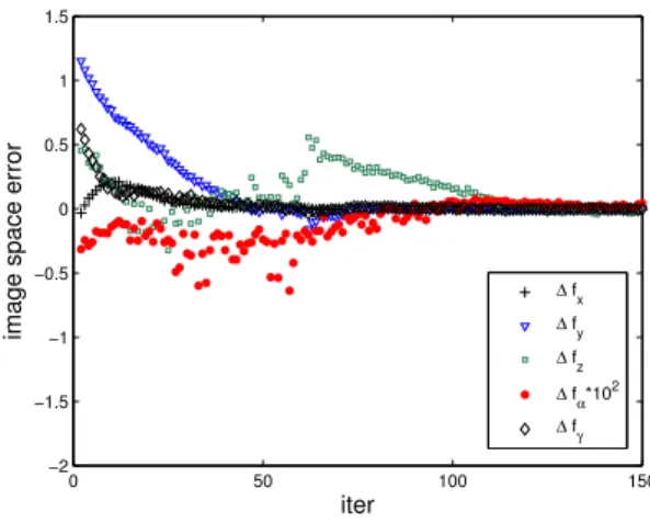
Figures 7 and 8 illustrate the evolution of the image and task space error for the exact Jacobian controller. The task space error does not decrease monotonically due to the inherent coupling between feature errors to multiple degrees of motion.

Both feature and task space error converge to a small residual error attributed to the image noise. The final task space error after 150 iterations is about ∆x = 0.75mm, ∆y = 1.2mm,

∆z = 0.5mm, ∆α = 0.65° and ∆γ = 1.5°. Figure 9

0 50 100 150

−2

−1.5

−1

−0.5 0 0.5 1 1.5

iter

image space error

∆ f_x

∆ f_y

∆ f_z*10

∆ f_α*10²

∆ f_γ

Fig. 7. Image space error of the Jacobian based controller

and 10 illustrate the behavior for the decoupled controller.

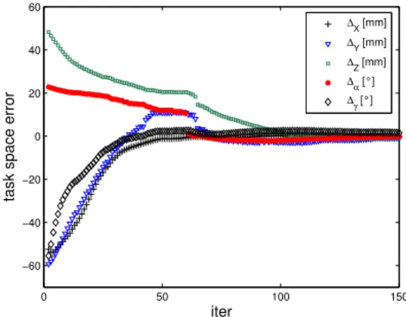
Notice, that the decoupled controller employs a feature f zσ

based on the scale of SIFT features rather than average distance between feature pairs. The feature errors converge smoothly except for the fluctuations in f zσ after about 50 iterations. The rapid increase in error is not caused by the control but the incorporation of additional SIFT features with

0 50 100 150

−60

−40

−20 0 20 40 60

iter

task space error

∆_X [mm]

∆_Y [mm]

∆_Z [mm]

∆_α [°]

∆_γ [°]

Fig. 8. Task space error of the Jacobian based controller

high frequency components that suddenly emerge for the first time as the camera zooms in onto the object. According to figure 4 their relative scale error is large, which results in an intermediate deterioration of the feature error that nevertheless is compensated in subsequent control steps. This observation is confirmed by the smooth progression of the task space error along the z-direction. The task space error evolves more smoothly as each degree of motion is governed by a single feature instead of being coupled to other features as well. The feature and task space errors converge to a final residual task space error in ∆x = 0.15mm, ∆y = 1mm, ∆z = 1mm.

The residual orientation error amounts to ∆α = 0.2° and

∆γ = 1.5°. This level of accuracy is more than sufficient for grasping and manipulation tasks in service robotics and even renders the control scheme possible for fine positioning of tools and objects in industrial applications. For the KATANA manipulator the final task space error is actually limited by the kinematic accuracy of the manipulator rather than the precision of visual control. The task space error evolves monotonically and more smoothly compared to the decoupled controller.

0 50 100 150

−2

−1.5

−1

−0.5 0 0.5 1 1.5

iter

image space error

∆ f_x

∆ f_y

∆ f_z

∆ f_α*10²

∆ f_γ

Fig. 9. Image space error of the decoupled controller

We also investigated the convergence behavior for the case

in which the feature plane in the reference pose and the image plane are no longer parallel. The computation of the image Jacobian assumes the same average depth z for all feature points as the centroid is considered equivalent to a single point feature. Therefore, the Jacobian based controller fails to converge to the reference pose for tilt angles of more than 30°. The decoupled controller is independent of a unique depth estimate and converges properly even for tilted feature planes.

This property allows arbitrary configurations between object and camera in the reference pose.

The experimental results demonstrate that it is possible to control a manipulator in 5-DOF with a monocular camera based on a decoupled controller without sacrificing robustness and accuracy performance with respect to the exact Jacobian based controller. It is also superior in terms of the smoothness of task space motion. The video sequences of the feature ex- traction and camera motion that are available at [12] illustrate the visual control with the decoupled controller.

0 50 100 150

−60

−40

−20 0 20 40 60

iter

task space error

∆_X [mm]

∆_Y [mm]

∆_Z [mm]

∆_α [°]

∆_γ [°]

Fig. 10. Task space error of the decoupled controller

VI. ^CONCLUSION

This paper presents a novel approach for visual servoing based on SIFT-features. The canonical keypoint orientation and scale of SIFT features enable direct control of the camera rotation around the optical axis and the translational along the z-axis. The visual features are generic as they are calcu- lated from moments of pixel coordinates, scale and keypoint orientation over a dynamic set of SIFT features. Thereby, the visual servoing control becomes entirely independent of the type of object and the visibility of specific features. The control scheme only relies on the dynamic subset of SIFT features that are reliably matched between the current and the reference image. This property adds to the robustness with respect to occlusion, change of view points and illumination.

It also enables a trade-off between computational complexity and accuracy by adapting the number of SIFT-features that are actually used for control. The image Jacobian for the visual features scale, orientation and centroids of SIFT-features is sparse with only minor couplings between the degrees of

motion. This property enables a simplified control scheme with one-to-one correspondence between degrees of motion and visual features. It is possible to further reduce the coupling by computing visual features as generalized geometric moments in which the weights are adapted in such a way that the cross-coupling terms disappear at the reference image. The decoupled controller operates with constant gains and does not require the online computation of the image Jacobian or its inverse. The computational demand for extracting and matching SIFT-features enable real time visual control at a frame rate of 7Hz. The experimental evaluation shows that the approach is reliable and efficient and achieves a final task space error in the order of a millimeter in translation and a degree in orientation.

In future work we intend to further investigate the concept of dynamically weighted moments proposed in section IV with the objective to entirely decouple visual features and motions.

Currently, the operational space of visual control is limited by the visibility and perceptibility of identical SIFT-features across different views. In our experience SIFT-features are still detectable at view point rotations of up to 30-40°. In order to accomplish large view visual servoing it is necessary to introduce additional intermediate reference views in order to successfully navigate across the entire view hemisphere.

Future research is concerned with the identification of interme- diate views and features and a heuristic for switching between reference SIFT features to achieve stable, robust and time- optimal camera motions in task space.

R EFERENCES

[1] S. Hutchinson, G. D. Hager, I. P. Corke, A Tutorial on Visual Servoing Control, IEEE Transactions on Robotics and Automation, vol.12, pp.651- 668, 1997.

[2] A.C Sanderson and L.E Weiss, Image-based visual servo control using relational graph error signals, Proceedings of the IEEE,pp. 1074-1077, [3] O. Tahri and F. Chaumette, 1980 Point-based and region-based image moments for visual servoing of planar objects, IEEE Transactions on Robotics and Automation, Vol. 21, No. 6, 2005.

[4] S. O. Belkassim, M. Shridhar, and M. Ahmadi, Shape-contour recognition using moment invariants, in Proc. 10th Int. Conf. Pattern Recog., Atlantic City, NJ, Jun. 1990, pp. 649-651.

[5] A. G. Mamistvalov, n-dimensional moment invariants and conceptual theory of recognition n-dimensional solids, IEEE Trans. Pattern Anal.

Machine Intell., vol. 20, no. 8, pp. 819-831, Aug. 1998.

[6] S. S. Reddi, Radial and angular moment invariants for image identifica- tion, IEEE Trans. Pattern Anal. Machine Intell., vol. PAMI-3, no. 2, pp.

240-242, Feb. 1981.

[7] D. G. Lowe, Distinctive image features from scale-invariant keypoints, International Journal of Computer Vision, 60, 2 (2004), pp. 91-110.

[8] A. Shademan and F. Janabi-Sharifi, Using scale-invariant feature points in visual servoing , Optomechatronic Sensors, Actuators, and Control, 2004, Proceedings of the SPIE, Volume 5603, pp. 63-70 (2004).

[9] O. Faugeras, Q.-T. Luong and T. Papadopoulu, The Geometry of Multiple Images, 2001, MIT Press.

[10] M. Iwatsuki, N. Okiyama, A new formulation of visual servoing based on cylindrical coordinate system with shiftable origin, in IEEE/RSJ Int.

Conf. on Intelligent Robots and Systems, IROS 02, October 2002.

[11] P.I. Corke and S.A. Hutchinson, A new partitioned approach to Image- Based Visual Servo Control, IEEE Transactions on Robotics and Automa- tion, Vol. 17,No. 4, 2001.

[12] http://www-rst.e-technik.uni-dortmund.de/dienst/de/content/Forschung

/Servicerobotik/PerformanceVideos.html