and Stock Market Contagion
Inauguraldissertation zur
Erlangung des Doktorgrades der
Wirtschafts- und Sozialwissenschaftlichen Fakult¨ at der
Universit¨ at zu K¨ oln
2013
vorgelegt von
Dipl.-Kfm. Claudio Nicolai Wewel aus
Stuttgart
Vorsitz: Univ.-Prof. Dr. Alexander Kempf, Universit¨ at zu K¨ oln
Tag der Promotion: 31. Januar 2014
The completion of this thesis would not have been possible without the support from many people, whom I would like to thank.
First, I would like to express my gratitude to Professor Thomas Hartmann-Wendels for taking the responsibility to supervise my thesis as well as for his guidance and continuous support. I would also like to thank him for the opportunity to present my work at several international conferences as well as his support for a research stay abroad. I would like to thank Professor Dieter Hess for serving as co-referee and Professor Alexander Kempf for chairing the dissertation committee.
I am greatly indebted to Professor Monika Trapp, who first attracted my interest to research on systemic risk. It has been a great pleasure working together. I am especially grateful for the numerous highly productive discussions with her that stimulated and deepened my interest in academic research as well as her continuous encouragement.
Moreover, I would like to thank Benjamin D¨ oring. I very much appreciate conducting joint research and am grateful for many fruitful discussions.
Many thanks go to my current and former colleagues at the University of Cologne.
In particular, I would like to mention Sebastian Bethke, Philipp Immenk¨ otter, Stefan Jaspersen, Stephan Nicklas, Sebastian Orbe, and Oliver Pucker for advice and valuable comments as well as David Fritz and Eugen T¨ ows for their helpfulness and advice – espe- cially with respect to L A TEX matters. I am grateful for the wonderful time spent together both on and off campus. Some research was completed in early 2013 during a research stay at Keio University in Tokyo, Japan. I am particularly grateful to Professor Naoyuki Yoshino for stimulating conversations and the friendly research environment. I gratefully acknowledge financial support from the University of Cologne and Keio University.
Finally, I wish to thank my family for their steady encouragement as well as their ideal and material support that made the completion of this work possible.
Cologne, February 2014 Claudio N. Wewel
Trapp, Monika and Claudio Wewel (2013). Transatlantic systemic risk. Journal of Banking & Finance 37 (11), 4241–4255.
D¨ oring, Benjamin, Thomas Hartmann-Wendels, and Claudio Wewel (2013). What can systemic risk measures predict? Working Paper.
Wewel, Claudio (2013). Are earthquakes less contagious than bank failures?
Comparative impact assessment of the Tohoku earthquake 2011 and the Lehman
bankruptcy 2008. Working Paper.
Front Matter vii
List of Tables . . . viii
List of Figures . . . . ix
1 Introduction 1 2 Transatlantic systemic risk 6 2.1 Introduction . . . . 6
2.2 Data . . . . 9
2.3 Measuring systemic risk . . . . 15
2.4 Results . . . . 19
2.4.1 Systemic risk within the US and Europe . . . . 20
2.4.2 Systemic risk between the US and Europe . . . . 25
2.4.3 Pre-crisis and crisis levels of systemic risk . . . . 27
2.4.4 The relation between banks and non-banks . . . . 31
2.5 Summary and conclusion . . . . 37
2.A Robustness issues . . . . 38
2.B Supplementary tables . . . . 41
2.C Time series diagnostics and goodness of fit . . . . 57
3 What can systemic risk measures predict? 65 3.1 Introduction . . . . 65
3.2 Data description . . . . 68
3.3 Systemic risk measures . . . . 71
3.3.1 Multi-period MES . . . . 71
3.3.2 SRISK . . . . 72
3.3.3 Multi-period CoVaR . . . . 73
3.4 Methodology . . . . 75
3.5 Results . . . . 78
3.5.1 Bank level . . . . 78
3.5.2 Banking system level . . . . 90
3.6 Summary and conclusion . . . 106
3.A DCC GARCH . . . 108
3.B Time series diagnostics . . . 109
4 Are earthquakes less contagious than bank failures? 112 4.1 Introduction . . . 112
4.2 Literature survey . . . 114
4.3 Data . . . 116
4.4 Methodology . . . 119
4.5 Results . . . 120
4.5.1 Contagious effects by industry . . . 120
4.5.2 Contagious effects by country . . . 128
4.6 Robustness issues . . . 129
4.6.1 Forbes-Rigobon correction for volatility . . . 129
4.6.2 Base criterion . . . 129
4.6.3 Comovement intensity . . . 134
4.7 Summary and conclusion . . . 137
4.A Principal components analysis and comovement intensity . . . 138
Bibliography 140
2.1 Summary statistics of the sample of CDS premia . . . . 12
2.2 Upper tail dependence within the United States and European banking sectors . . . . 22
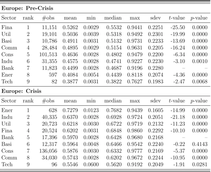
2.3 Upper tail dependence coefficients between US and European banking sectors 26 2.4 Pre-crisis and crisis upper tail dependence within and between the US and European banking sectors . . . . 29
2.5 Upper tail dependence between the banking and non-bank sectors within the United States and Europe . . . . 33
2.6 Upper tail dependence between small/large banks and non-banks within the United States and Europe . . . . 36
2.7 Robustness with respect to length of times series . . . . 38
2.8 Robustness with respect to Wilcoxon test . . . . 39
2.9 Intra-sectoral upper tail dependence coefficients by geographical region . . 41
2.10 Upper tail dependence between Europe and the United States by sector . . 42
2.11 Pre-crisis and crisis levels of intra-sectoral upper tail dependence coeffi- cients by geographical region . . . . 44
2.12 Inter-sectoral upper tail dependence coefficients by geographical region . . 45
2.13 Inter-sectoral upper tail dependence coefficients by geographical region . . 46
2.14 Intra- and inter-sectoral upper tail dependence coefficients (United States) 49 2.15 Intra- and inter-sectoral upper tail dependence coefficients (Europe) . . . . 53
2.16 Description of banks . . . . 55
2.17 CDS notional volume by currency . . . . 56
2.18 Time series properties of CDS bid quotes: p-values . . . . 57
2.19 Goodness of fit of the extreme value distribution: p-values . . . . 59
2.20 Goodness of fit of the extreme value distribution: Log-likelihood values . . 60
2.21 Goodness of fit of the Gumbel copula: p-values . . . . 61
2.22 Goodness of fit of the Gumbel copula: Log-likelihood values . . . . 62
2.23 Auto-correlation of upper tail dependence coefficients series: p-values . . . 63
3.1 Bank characteristics and descriptives . . . . 69
3.2 Summary of bank balance sheet characteristics . . . . 70
3.3 Statistics on weekly systemic risk estimates (Subprime Crisis 2008) . . . . 79
3.4 Statistics on weekly MultiMES estimates (Euro Crisis 2011) . . . . 82
3.5 Determinants of systemic risk at the bank level . . . . 89
3.6 Description of variables employed in the VAR models . . . . 91
3.7 VAR results (full sample) – Part I . . . . 97
3.8 VAR results (full sample) – Part II . . . 100
3.9 VAR results (July 2005 – June 2009) . . . 103
3.10 VAR results (July 2009 – June 2013) . . . 105
3.11 Time series diagnostics (first differences): p-values and test statistics . . . 110
3.12 Diagnostics of sample bank’s daily log return series: p-values and test statistics . . . 111
4.1 Sample composition by country and industry . . . 117
4.2 Cross-market correlations by industry (international, incl. event country) . 122 4.3 Cross-market correlations by industry (event country) . . . 123
4.4 Cross-market correlations by industry (international, excl. event country) . 126 4.5 Cross-market correlations by country (international) . . . 127
4.6 Robustness: Cross-market Forbes-Rigobon (2002) correlations by industry 130 4.7 Robustness: Cross-market Forbes-Rigobon (2002) correlations by country . 131 4.8 Robustness with respect to base criteria, by industry . . . 132
4.9 Robustness with respect to base criteria, by country . . . 133
4.10 Robustness: Comovement intensity by industry . . . 135
4.11 Robustness: Comovement intensity by country . . . 136
2.1 Time evolution of CDS premia averaged across sectors (United States) . . 14
2.2 Time evolution of CDS premia averaged across sectors (Europe) . . . . 14
2.3 Time evolution of upper tail dependence within the regional banking sectors 20 2.4 Time evolution of intra-sectoral upper tail dependence (United States) . . 24
2.5 Time evolution of intra-sectoral upper tail dependence (Europe) . . . . 24
3.1 Time evolution of MultiMES . . . . 85
3.2 Time evolution of SRISK . . . . 85
3.3 Time evolution of ∆MultiCoVaR . . . . 86
3.4 Time evolution of risk measures . . . . 93
3.5 Time evolution of bank balance sheet variables . . . . 94
3.6 Time evolution of financial market variables . . . . 95
3.7 Time evolution of macro-economic variables . . . . 96
4.1 Time evolution of daily S&P 500 and NIKKEI 225 index levels . . . 118
“The game of science is, in principle, without end. He who decides one day that scientific statements do not call for any further test, and that they can
be regarded as finally verified, retires from the game.”
– Sir Karl R. Popper
The recent Subprime and Euro Crises have stressed the vulnerability of the international banking system and the adverse impact that bank defaults have on the macro-economy.
Over the last decades, financial markets (and in particular banks) have become increas- ingly interconnected as a result of financial liberalization, growing international trade, and increasingly global supply chains. In this effect, the understanding of systemic risk and financial contagion that pose a threat to both the international financial system and to the real economy (through its dependence on the financial sector) is of vital interest to both researchers and economic policy makers.
Over the years, various definitions of systemic risk and contagion have emerged. Ac- cording to the 2001 Report on Consolidation in the Financial Sector, the Group of Ten (2001) defines systemic risk as follows:
Systemic financial risk is the risk that an event will trigger a loss of economic value or confidence in, and attendant increases in uncertainly about, a sub- stantial portion of the financial system that is serious enough to quite probably have significant adverse effects on the real economy. Systemic risk events can be sudden and unexpected, or the likelihood of their occurrence can build up through time in the absence of appropriate policy responses. The adverse real economic effects from systemic problems are generally seen as arising from disruptions to the payment system, to credit flows, and from the destruction of asset values.
The previous definition provides a general and intuitive insight to the notion of sys- temic risk. Thus, more concisely, systemic risk can be subsumed as the risk or the proba- bility of breakdowns in an entire system, as opposed to breakdowns in individual parts or components, and is evidenced by comovements (correlation) among most or all the parts (Kaufman and Scott, 2003).
In literature, there is consesus that two alternate main mechanisms cause systemic risk:
common shocks (e.g., Kaufmann, 2000; Helwege, 2010) and contagion (e.g., Lando and
Nielsen, 2010; Longstaff, 2010). Contagion requires strong interconnectedness between
financial institutions such as mutual credit exposures or derivatives transactions entailing
counterparty risk and may occur if an institution I defaults on payments to another
institution J (that is closely connected to I) causing J to default on its own payments
and thereby potentially causing financial distress of further institutions. More generally,
Kaminsky and Reinhart (2000) refer to contagion as channels through which disturbances are transmitted and mention trade links and (largely ignored) financial sector links such as bilateral exposures and interbank loans as examples.
Whereas contagion refers to a direct causation mechanism, causation by common shocks is rather indirect. Moreover, causation by common shocks necessitates sufficiently homogenous risk factors, i.e., similarities in the financial institutions’ portfolios. Thus, if insitutions’ risk exposures are alike, a shock resulting in severe losses to an asset could result in uncertainty about similar traded assets potentially subject to the same shock (Kaufmann, 2000). Given that these assets constitute a substantial portion in a multitude of financial institutions’ portfolios, such a shock could potentially trigger simultaneous losses to a wide range of institutions with similar exposures across the financial industry.
Research on systemic risk can be separated into various branches. One branch focuses on general systemic risk measurement and can furthermore be systemized as follows:
(i) Asset price based measurement. Over the past years, the Conditional Value at Risk (Adrian and Brunnermeier, 2011) and the Marginal Expected Shortfall (Acharya et al., 2010) have emerged as the most prominent asset price based measures. The latter measures are applied by the U.S. Treasury Department (Financial Stabil- ity Oversight Council, 2013) and the European Systemic Risk Board (European Systemic Risk Board, 2013) and have triggered numerous studies proposing exten- sions. 1 Other approaches proposed by academia are based on extreme value theory (De Jonghe, 2010; Zhou, 2010), principal component analysis (Billio et al., 2012;
Kritzman et al., 2011), and default probabilities (Lehar, 2005; Huang et al., 2009;
Segoviano and Goodhart, 2009; Huang et al., 2012; Gray and Jobst, 2010).
(ii) Network analysis based measurement. This strand of literature analyzes systemic risk modeling institutions’ mutual exposures (e.g., Elsinger et al., 2006a; Allen et al., 2010; Tarashev et al., 2010; Halaj and Kok Sorensen, 2013).
An advantage of network based modelling is that such an analysis may even incorporate institutions whose stock is not traded on stock markets. 2 However, this comes at the cost
1
Several studies implement the Marginal Expected Shortfall (Acharya and Steffen, 2012; Idier et al., 2013), related measures (Engle et al., 2012; Acharya et al., 2012), and the Conditional Value at Risk (L´ opez-Espinosa et al., 2012; Van Oordt and Zhou, 2011; Roengpitya and Rungcharoenkitkul, 2011;
Gauthier et al., 2010). Other studies propose various extensions to the latter approaches (Hong, 2011;
Girardi and Erg¨ un, 2013; Cao, 2013).
2
This concern particularly applies to economies with few publicly traded banks such as Germany or
Austria.
of employing balance sheet data with much lower sampling frequency than stock prices.
Thus, asset price based measures are capable of reflecting the daily dynamics at the stock markets. Moreover, asset price based measures are less likely to be prone to national particularities in accounting practices and hence allow for broad analyses and comparisons within the international banking system. Bisias et al. (2012) provide an extensive survey on the literature on systemic risk measurement.
Another branch investigates common shocks and contagion in an event study setup.
Research on contagion is abundant with literature covering financial crises such as the Mexican Peso Crisis in 1994 (e.g., Calvo and Reinhart, 1996; Edwards, 1998) or the Sub- prime Crisis including the bankruptcy of Lehman Brothers (e.g., Longstaff, 2010; Hwang et al., 2010; Bekaert et al., 2011) as well as contagion following Black Swan events such as the 1987 Black Monday (e.g., King and Wadhwani, 1990; Hamao et al., 1990; Bertero and Mayer, 1990) and the September 11, 2011 terrorist attacks (e.g., Hon et al., 2004) or natural disasters (e.g., Lee et al., 2007; Asongu, 2012).
This thesis consists out of three essays on systemic risk in the banking system and stock market contagion. The first essay (Trapp and Wewel, 2013, ”Transatlantic systemic risk”) investigates which type of systemic risk – common shocks or contagion – dominated in the banking system at the onset of the Subprime Crisis and thus contributes to the literature on the distinction of contagion and common shocks.
Applying a Copula approach, we measure bivariate upper tail dependence between CDS premia of 550 firms based in the US and Europe. We show that banks’ exposures to common risk factors are crucial for systemic risk in the banking sector. We come to this conclusion by showing that dependencies are generally higher within the US and Europe than between these regions. At the onset of the Subprime Crisis, however, systemic risk in Europe increases much more strongly than in the US. Given that intra-regional depen- dencies are stronger than transatlantic dependencies, we argue that the steep increase of systemic risk in Europe is unlikely to arise from contagion but rather from common risk factors in the banks’ portfolios.
We furthermore find that dependence between banks and real sector firms is limited,
however, European banks are more closely connected to real sector firms of the same
region than their US counterparts. This finding is likely to result from a relatively higher
importance of bank loans as a means of funding to European real sector firms when
compared to US firms that rely on capital market-based funding to a greater extent (see,
e.g., Demirguc-Kunt and Levine, 1999).
Our results indicate that in the Subprime Crisis, common factors played a much more important role than contagion, which is in line with the findings of Kaufmann (2000). Our results have important implications for regulatory authorities stressing the importance of monitoring international bank dependencies arising from common risk factors. Moreover, the limited dependencies between banks and real sector firms imply that while regulators should pay particular attention to large banks providing a substantial share of loans to real-sector firms, they should improve real sector firms’ access to the capital markets.
The second essay (D¨ oring, Hartmann-Wendels, and Wewel, 2013, ”What can sys- temic risk measures predict?”) contributes to the literature on the assessment of systemic risk measures and to the literature on CoVaR (Adrian and Brunnermeier, 2011), MES (Acharya et al., 2010), and the related SRISK measure (Brownlees and Engle, 2012). 3 In a first step, we implement these three prominent systemic risk measures in a DCC GARCH framework.
Systemic risk measures should be able of capturing distress in the banking system that subsequently leads to substantial downturns in the real economy. Hence, in a second step, we compare the measures evaluating their adequacy as a tool for regulatory authorities on the basis of their predictive power for various market, balance sheet related, and macro- economic variables investigating directionalities at the bank as well as at the banking system level. We apply the measures to a sample of stock prices of European banks with total assets above e 30bn in the period from July 2005 to June 2013. 4 As European banks are likely to be affected by both the recent international financial crisis and the European sovereign debt crisis, the European banking system constitutes a unique setting for the assessment of systemic risk measures. Moreover, we ensure that the systemic risk measures are not exclusively evaluated by their performance during the Subprime Crisis.
Overall, we find that systemic risk measures are capable of capturing early symp- toms of distress in the financial markets. Furthermore, we find that at the banking system level systemic risk measures possess substantial forecasting power for a variety of
3
Literature on the CoVaR, MES, and SRISK measures can be systemized as follows: (i) studies employing CoVaR (L´ opez-Espinosa et al., 2012; Van Oordt and Zhou, 2011; Roengpitya and Rungcharoenkitkul, 2011; Gauthier et al., 2010) and MES related measures (Acharya and Steffen, 2012; Idier et al., 2013; Engle et al., 2012; Acharya et al., 2012) to analyze distress in the financial markets (ii) extentions of the latter measures (Hong, 2011; Girardi and Erg¨ un, 2013; Cao, 2013), and comparisons between the latter (Jiang, 2012; Benoit et al., 2013; L¨ offler and Raupach, 2013).
4
According to the European Commission’s proposal for a Single Supervisory Mechanism (SSM) for the
European Banking Union, banks with total assets above e 30bn are supervised directly by the ECB
due to their potential systemic relevance (European Commission, 2013).
financial market variables (EURIBOR-OIS spread and volatility), balance sheet variables (leverage, market-to-book ratio, and profitability), and macro-economic variables (GDP, housing prices, and economic sentiment). Whereas balance sheet characteristics determine an individual bank’s systemic importance, they cannot explain or predict systemic risk at the banking system level. Comparing the predictive power of the analyzed measures, we find that the CoVaR’s forcasting power is dominated by MES related measures’ predictive power and conclude that the latter are thus most suitable for regulatory purposes.
The third essay (Wewel, 2013, ”Are earthquakes less contagious than bank failures?
Comparative impact assessment of the Tohoku earthquake 2011 and the Lehman bank- ruptcy 2008”) contributes to the literature on international stock market contagion. Em- ploying a data set of 4,350 international stocks in 13 countries, we investigate pre-and post-event cross-market correlation on national and international stock markets following the Japanese Tohoku 5 earthquake on March 11, 2011, the subsequent tsunami and the nuclear disaster at Fukushima Daiichi. To better evaluate the degree of contagion, we employ the bankruptcy of Lehman Brothers on September 15, 2008 as benchmark event.
Contrary to previous studies (Lee et al., 2007; Asongu, 2012), we analyze contagion by in- dustry and country at the individual share price level which allows us to explore potential geographical patterns of how contagion propagates through global stock markets.
Overall, we find that contagion arising from both events is substantial. Whereas the Lehman bankruptcy affected stocks from all industries globally, the Tohoku earthquake only significantly affected insurance and utilities stocks. We argue that the degree of global stock markets’ response is explained by distinct contagion mechanisms. Events such as the Lehman bankruptcy have the potential to result in panics at the global stock markets, which emerge as a consequence of anticipated future losses resulting from financial exposures or future liquidity freezes. As global stock markets are higly integrated, such panics are easily transmitted. Contrary, natural disasters are less likely to be followed by panics because stock market participants will anticipate price effects to have fully materialized after the disaster. Moreover, the destruction of (real) assets will be most severe in the event country itself. International supply chain disruptions arising from destroyed production facilities impact global stock only to a lesser degree.
5
The term Tohoku refers to the Northeast of Japan’s main island Honshu and represents the region
that was most severely affected by the earthquake.
2.1 Introduction
Where does systemic risk come from, and how should we regulate it? The first, most commonly cited mechanism causing banks to default jointly is contagion: Banks can be connected with one another because of direct bilateral exposures, e.g., through interbank loans or derivatives transactions entailing counterparty risk. In this case, regulation must specify limits to the exposure one bank can have towards another to prevent one default from causing a meltdown of the entire banking system. Second, if banks hold similar portfolios, a common shock may simultaneously affect all banks and also lead to the joint default of multiple banks. Then, the main role of regulation is to ensure that there is sufficient variation across the portfolios of different banks, or at least variation in the sensitivities of the portfolio values towards joint risk factors.
Both of these channels for systemic risk, contagion and conditional independence, have been discussed in the literature on joint defaults (see, e.g., Lando and Nielsen, 2010;
Longstaff, 2010). However, evidence on which type of systemic risk dominates in the banking system is extremely scarce for three reasons. First, information at the portfolio level is, if at all, only available to supervisory authorities. Second, even supervisors of- ten do not have disaggregate information on mutual exposures at the international level.
Hence, the only study differentiating between common shocks and bilateral exposures that we are aware of analyzes US data (Helwege, 2010). An international setting, however, is crucial because distinguishing between a common shock and one originating within an individual bank is almost impossible at the national level. Third, even if they were avail- able, portfolio-level information may not sufficiently reflect interbank exposures. Given most banks’ limited exposures 1 towards Lehman, it is unlikely that balance-sheet based measures of systemic risk could have quantified the resulting declines of bank stocks and defaults of numerous financial institutions.
In this study, we explore whether systemic risk arises from common shocks or contagion in an international setting. We focus on the two largest integrated economic regions in the world, the United States of America and Europe, because each constitutes an integrated
1
While Bank of America filed a 5.3 bn USD claim against Lehman, followed by Goldman with 2.5
bn USD, Bloomberg estimated the aggregate exposure for European banks and insurers to lie below
7.3 bn USD shortly after Lehman filed for bankruptcy on September 15, 2008. “European Banks,
Insurers Have $7.3 Billion Exposure to Lehman”, Fabio Benedetti-Valentini and Elisa Martinuzzi,
September 18, 2008.
banking market with homogenous regulation and a single predominant currency. We avoid the issue of obtaining portfolio exposures or balance sheet information by using the prices of traded assets, and directly infer systemic risk by adapting the copula approach of Buehler and Prokopczuk (2010) to credit default swap (CDS) premia.
We explore the importance of common shocks vs. contagion for the banking sector in two steps. First, we document that connections between US and European banks are low compared to those within each region. Second, we show that the onset of the Subprime Mortgage Crisis increased systemic risk in Europe much more strongly than in the US. This effect strongly points at a prevalence of common shocks: An increase in subprime mortgage loan defaults in the US is a local shock (as, for that matter, the Lehman bankruptcy). Since the connection between US banks is stronger than between US and European banks, a transmission of this shock through contagion would imply that systemic risk should increase less strongly in Europe than it does in the US.
We then turn to the implications of banking risk for the real sector. During the recent financial crisis, banks received financial support under the troubled asset relief program (TARP), the European Financial Stability Facility (EFSF), and the European Financial Stabilisation Mechanism (EFSM) due to concerns about a recession arising from another bank’s default. This concern was well-grounded in historical experience, even prior to the Lehman bankrupcty: As Reinhart and Rogoff show in a series of papers (2009c, 2009a, 2009b), banking crises are regularly followed by a drop in equity prices, output, and employment levels since real-sector firms rely on banks as a source of external funding.
We therefore determine how strongly banks and firms from a wide range of real sectors are connected, again by applying the copula approach to CDS premia for these firms. This allows us to base our analysis on a large range of firms besides banking and insurance, for which regulatory guidelines demand publication of balance sheet information at an extremely detailed level (see, e.g., Furfine, 2003; Wells, 2004; Gauthier et al., 2010).
Interestingly, we find that banks do not play a central role: Firms from a given real sector are more strongly connected to both firms from the same real sector and to firms from any other real sector than they are to banks. Only other banks and non-bank finan- cial firms are more strongly connected to banks than to real-sector firms. At first sight, this result appears surprising, because of the established role of banks in supplying loans to the real sector. However, the importance of banks in this respect can vary substantially.
For example, a large group of small banks on average provides more loans than a small
group of large banks, and banks with a larger focus on investment banking provide fewer
loans than banks with a strong focus on commercial banking (Altunbas et al., 2002; Jia,
2009). Most banks in our sample are large, international banks. Therefore, our results
imply that the default of a single large real-sector firm is more likely to lead to a recession than the default of a large, international bank.
In addition to the differentiation between common shocks and contagion, our study contributes to several strands of literature. First, we extend the broad body of literature on systemic risk for financial institutions. Studies that compare banks to other financial institutions (see, e.g., Billio et al., 2012; Bosma et al., 2012) mostly find that systemic risk is highest for banks. Very few studies (see, e.g., Harmon et al., 2010; Muns and Bijlsma, 2011; Buehler and Prokopczuk, 2010) compare systemic risk in the banking sector to systemic risk for non-financial firms, and come to the same conclusion: systemic risk is highest in the banking sector. We extend this literature by showing that the interdependence between banks and non-banks is low, compared to systemic risk within and between real sectors.
Studies analyzing the determinants of systemic risk identify bank size, interbank loan ratio, and the bank’s country of origin (Elsinger et al., 2006a), linkages at the asset level and mutual credit relations (Elsinger et al., 2006b), and the bank’s default probability (Huang et al., 2012) at the individual level as significant factors. We contribute to this literature by showing that the link between non-banks and banks is higher in Europe than in the US. This is in line with the greater importance of banks as a source of external financing in Europe (see, e.g., Demirguc-Kunt and Levine, 1999; Dermine, 2002; Kwok and Tadesse, 2006).
From a macro perspective, Kaminsky and Reinhart (1999) argue that a typical banking crisis begins with a period of financial liberalization, leading to an economic boom and an overvaluation of the local currency, which leads to a recession and a reinforcing banking and currency crisis. Multiple studies have explored this mechanism empirically, and come to the conclusion that adverse economic conditions coincide with higher systemic risk (see, e.g., Buehler and Prokopczuk, 2010; Bartram et al., 2007), and regions differ significantly regarding their susceptibility to contagion (Bae et al., 2003). In contrast, Bosma et al.
(2012) study global relations between financial firms, and find that systemic risk has uniformly decreased since the onset of the financial crisis. We contribute on this macro perspective by showing how the financial crisis has intensified systemic risk in the US and Europe.
Second, we contribute to the literature on international relations between financial
firms. The global banking system has become more integrated within the last 30 years
(Garratt et al., 2011) for a variety of reasons: In addition to the active interbank markets,
banks have branched out from their domestic to foreign markets, and the liberalization of
financial markets has led to the creation of new financial products. As a result, banks are
exposed to similar risk factors globally. However, these global factors do not obliterate the importance of regional factors (Bartram et al., 2007). Consistent with evidence by Hartmann et al. (2006) for banks in different EMU countries, we find higher financial integration within the US and within Europe than between the two regions. We also document the evolution of these differences over time, and show that they drastically decrease during the financial crisis.
Last, our results have implications for the structure of international financial regula- tion. For example, Went (2010) discusses the implications of the new focus on systemic risk in the Basel III framework, and Hanson et al. (2011) develop a framework for macro- prudential instead of microprudential regulation. Blackmore and Jeapes (2009) study the consequences of one global financial regulator compared to a multi-regulator approach under international guidelines. Our results have two implications for this body of litera- ture. First, monitoring exposures towards common shocks at the international level is a central issue no less important than monitoring bilateral exposures. Second, bailouts for large international banks which are termed ”too big to fail” are not necessary to avoid spillovers to the real sector if the bilateral exposures between these banks and smaller banks supplying the majority of loans are properly monitored.
The remainder of the paper is structured as follows: In Section 2.2, we give an overview over the CDS time series used to compute systemic risk. We motivate and develop our systemic risk measures in Section 2.3, and present the empirical results of our study in Section 2.4. Section 2.5 summarizes and concludes.
2.2 Data
In our analysis, we use CDS premia to determine systemic risk. Clearly, the use of CDS premia instead of stock returns or equity option data has advantages and disadvantages.
On the one hand, the CDS premium has a closer link to a firm’s default than stock returns.
For example, stocks frequently trade at a non-zero price even after the underlying firm has defaulted on debt payments. This effect points at violations of the absolute priority rule, which has been documented by Unal et al. (2003). On the other hand, CDS might also reflect factors other than the underlying entity’s default risk. We believe that illiquidity, the delivery option, and counterparty risk play a particular role:
(i) Lower liquidity in the CDS market will be associated with lower bid quotes. Hence,
our systemic risk estimate which is derived via the upper tail dependence is unlikely
to be upwards-biased due to deteriorating liquidity conditions in the CDS market.
For CDS ask quotes, the opposite effect prevails. Buehler and Trapp (2010) show that the effect of CDS liquidity on CDS quotes can be substantial.
(ii) Both CDS bid and ask quotes may be biased upwards or downwards because of counterparty risk, depending on whether the protection seller’s or the protection buyer’s default is more likely. 2 As Arora et al. (2012) show, counterparty risk has a very limited effect on CDS premia of around 1 bp. 3 Hence, fluctuations of counterparty risk are likely to have almost no effect on CDS premia overall.
(iii) A protection buyer has the option to deliver the cheapest out of a range of bonds after a default of the underlying reference entity. This cheapest-to-deliver option should increase both CDS bid and ask quotes.
Overall, CDS bid quotes are less likely to increase for reasons other than fundamental default risk, compared to CDS ask quotes. An upper tail dependence estimate derived from CDS bid quotes will thus be more conservative than an estimate derived from CDS ask quotes. We attempt to minimize the impact of these alternative sources of CDS premium variation by focusing on the CDS bid quote.
We obtain our CDS data from Bloomberg. We focus on the five-year maturity and use Credit Market Analysis (CMA) as our price source, since Mayordomo et al. (2010) show that new information seems to be reflected most quickly for this maturity-provider combination. To ensure comparability between the CDS contracts, we focus on CDS written on senior unsecured debt.
Overall, Bloomberg specifies the following sectors: Basic Materials, Communication, Consumer (Cyclical), Consumer (Non-cyclical), Diversified, Energy, Financial, Sovereign, Industrial, Technology, Utilities. We perform four modifications: First, we merge the cyclical and the non-cyclical consumer sectors. 4 Second, we manually verify whether firms with the “Financial” sector tag are banks or non-banks, 5 and split the ”Financial” sector accordingly. Third, we drop CDS contracts written on firms from the “Diversified” sector since only twelve firms, mostly holding companies, fall into this category. Last, we drop
2
To be precise, both the univariate default risk of protection buyer and seller as well as their joint default risk with the underlying reference entity matter for the total effect.
3
This is likely due to the margin payments that are regularly made in most CDS contracts as the contract value changes over time.
4
This merge ensures comparability between Bloomberg and Industry Classification Benchmark (ICB) sectors.
5
We define a bank as a financial institution with the authority to accept deposits and grant loans. Such
an institution may of course also operate outside of this area, e.g., offer asset management services.
all CDS contracts written on reference entities termed “Sovereign”, since the economic rationale behind joint defaults of sovereign reference entities (such as municipalities or states) is likely to be different than for non-sovereign firms. This leaves us with 1,323 firms.
We split our sample into the following two (regulatory) regions: the United States of America (US) and Europe. For 957 of the 1,323 firms, we are able to identify the country of the firms’ headquarters. 550 out of the 957 firms are headquartered either in the US or in Europe. The subsample used for the following analysis contains 335 firms for the US and 215 firms for Europe, including the UK. 6 For these 550 firms, we collect daily CDS bid quotes, denominated in basis points per annum, via Bloomberg from October 2004 to October 2009, omitting all zero quotes. 7 Table 2.1 reports descriptive statistics of all CDS contracts in our final sample.
As Panel A of Table 2.1 shows, the number of firms is not evenly distributed across sectors with only 19 firms in the technology sector, and 173 firms in the consumer sector.
The joint financial sector (bank and non-bank) is the second-largest sector with 103 firms, of which 35 are banks. With a total of 65,950 observations for these banks, we are confident that the CDS premia with a mean of 95 bp and a standard deviation of 305 bp are a reliable indicator of default risk in the banking sector. The strongly skewed distribution of CDS premia (the median on average amounts to one third of the mean) indicates that a symmetric dependence measure would severely underestimate upper tail dependence. 8
6
The exact composition of the subsample (i.e., the distribution of firms among countries within both considered regions) is as follows:
US (335 firms) ; Europe (215 firms) – Austria (2), Belgium (3), Denmark (5), Finland (5), France (39), Germany (29), Greece (2), Ireland (3), Italy (12), Netherlands (11), Norway (2), Portugal (2), Spain (10), Sweden (14), Switzerland (13), United Kingdom (63). We include Norway and Switzerland in the region Europe even though they are not members of the European Union since they implemented Basel II along the Directives 2006/48/EC and 2006/49/EC of the European Parliament and the Council, and are adopting the new Basel III directives, such that the region Europe has a homogenously regulated banking sector.
7
To explore whether our results are affected by possibly stale premia, we repeat our analyses on a subset of CDS premia where all quotes that do not exhibit a change within a week are omitted. The results are virtually identical.
8
The high maximum values in our sample are due to the fact that a number of firms default during the
observation interval. For example, Clear Channel Communications, Inc., a media and entertainment
company, experienced a distressed exchange default in August 2009. Loss given default estimates
from Moody’s for senior unsecured bonds were as high as 92%. Consequently, CDS premia for Clear
Channel Communications increased to 9,580.20 bp.
P anel A – Complete Sample CURRENCY (in %) MO M E N T S QUANTILES Sector (abbr.) #firms EUR GBP USD #obs mean sdev min q = 0 . 25 q = 0 . 50 q = 0 . 75 m ax Basic Materials Basi 47 3 4.04 2.13 63.83 77,668 156.09 399.71 6.81 28.00 53.33 130.51 5,316.67 Comm unicatio n Comm 52 53.85 3.85 42.31 82,245 192.29 421.99 6.95 39.55 72.75 193.40 9,580.20 Consumer Con s 173 32.95 2.89 64.16 287,118 190.26 5 09.57 1.67 29.36 60.00 164.21 9,135. 45 Energy Ener 35 11.43 – 88.57 55,795 95.97 128.50 2.36 26.50 41.11 101.85 1,009.25 Financial (Bank) Bank 35 65.71 – 34.29 65,9 50 95.47 305.03 2.17 11.25 22.00 80.52 5,886. 42 Financial (Non-Bank) Fina 68 32.35 2.94 64.71 106,490 184.45 417.48 3.63 23.84 43.27 138.87 6,274.24 Industrial Indu 78 39.74 – 60.26 133,761 97.17 186.43 5.7 5 25.38 45.00 106.00 5,165.69 T ec hnology T ec h 19 10.53 – 89.47 25,918 168.38 365.08 4.0 0 24.77 61.70 120.33 4,632.01 Utilities Util 43 48.84 2.33 48.84 75,583 69.82 95.96 4.3 5 23.50 38.50 68.32 1,011.13 ALL 550 37.09 2.00 60.91 910,528 149.91 389.30 1.67 25.50 49.36 127.70 9,580.20 P anel B – United States Sample Basic Materials Basi 29 – – 100.00 44,823 193.55 502.66 6.8 1 32.25 64.30 172.77 5,316.67 Comm unicatio n Comm 22 – – 100.00 29,0 90 267.10 621.95 8.87 44.53 91.51 23 4.00 9,580.20 Consumer Con s 112 0.89 – 99.11 179,7 17 227.98 624.67 3.00 29.04 62.56 17 9.99 9,135.45 Energy Ener 31 – – 100.00 47,5 15 106.39 134.87 5.00 28.25 45.15 11 9.75 1,009.25 Financial (Bank) Bank 12 – – 100.00 23,461 167.88 4 84.16 5.03 20.23 32.17 114.70 5,886. 42 Financial (Non-Bank) Fina 44 – – 100.00 63,779 228.47 488.55 6.06 27.58 49.33 192.50 6,274.24 Industrial Indu 47 – – 100.00 74,5 45 88.84 128.92 5.75 23.67 45.49 105.25 1,965.16 T ec hnology T ec h 17 – – 100.00 21,8 69 184.52 394.65 4.00 23.00 60.03 12 5.09 4,632.01 Utilities Util 21 – – 100.00 33,4 08 80.24 99.50 7.10 33.57 45.45 75.86 760.10 ALL 335 0.30 – 99.70 518,207 182.01 483.76 3.00 28.00 53.95 144.50 9,580.00 P anel C – Europ ean Sample Basic Materials Basi 18 8 8.89 5.56 5.56 32,8 45 104.98 168.75 6.99 23.68 43.33 85.00 1,855.30 Comm unicatio n Comm 30 93.33 6.67 – 53,155 151.36 243.12 6.95 38.31 62.33 162.50 3,076.72 Consumer Con s 61 9 1.80 8.20 – 107,401 127.16 186.62 1.67 29.70 57.19 146.70 2,352.70 Energy Ener 4 100.00 – – 8,280 36.20 52.00 2.36 8.44 20.96 41.22 483. 23 Financial (Bank) Bank 23 100.00 – – 42,489 55.49 102.45 2.1 7 9.33 13.60 7 0.43 1,113.75 Financial (Non-Bank) Fina 24 91.67 8.33 – 42,711 118.72 266.32 3.6 3 18.12 31.00 95.25 4,341.46 Industrial Indu 31 100.00 – – 59,2 16 107.65 239.56 7.00 27.50 44.50 10 8.43 5,165.69 T ec hnology T ec h 2 100.00 – – 4,049 81.22 54.42 19.5 6 30.11 72.50 115.00 283.64 Utilities Util 22 95.45 4.55 – 42,175 61.57 92.24 4.35 19.54 28.73 62.98 1,011. 13 ALL 215 94.42 5.12 0.47 392,321 107.51 1 98.65 1.67 22.54 44.00 107.80 5,165. 69 T able 2.1 – Summary stati stics of the sample of CDS premia The ab o v e table presen ts descriptiv e statistics on the time series of daily CDS premia used in our analysis. All CDS data are obtained via Blo om b erg; the time series of obse rv ations ranges from Octob er 2004 to Octob er 2009.
Table 2.1 – continued:
To minimize the impact of factors other than the underlying reference entity’s default risk, we only consider bid quotes. In total, we have 5-year CDS contracts on 550 firms in our sample, all of which are on senior unsecured debt. Panel A presents descriptive statistics of the entire sample and Panels B and C provide statistics by region. Column two gives the sectoral abbreviations used in the remainder of this paper, column three the number of available firms for each sector, columns four to six the relative distribution of CDS contracts across currencies; column seven gives the number of observations used to compute mean and standard deviation in columns eight and nine; columns ten to fourteen present the quantiles. Appendix-Table 2.16 presents the names of the US and European banks in our sample and Appendix-Table 2.17 provides supplementary information on the CDS market.
Regarding the US and European sub-samples in Panels B and C of Table 2.1, we find that CDS contracts for US firms are almost exclusively denominated in US-Dollar (USD). Our sample contains 12 US banks, which have a significantly higher average CDS premium of 168 bp compared to their 23 European counterparts with an average of 55 bp.
We take this difference as an indication that aggregate risk (not dependence) is higher for US banks than for European ones.
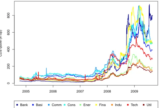
In Figures 2.1 and 2.2, we present the time series of CDS premia, taking cross-sectional averages across all CDS premia for firms in the same sector on each observation date. We separately display the averages for the US and Europe.
Figures 2.1 and 2.2 allow for two main observations. First, CDS premia in the different sectors evolve similarly over time both in the US and in Europe until mid-2008. Around the time of the Lehman default, CDS premia begin to evolve very differently in the US and in Europe. In the US, we observe a drastic increase for banks and non-bank financial firms. In Europe, the increase is strongest for non-bank financial and industrial firms.
For the latter, we attribute the increase to automotive firms subsumed in the industrial sector. Banks, on the other hand, exhibit CDS premia in the intermediate range.
Our second observation concerns the comovement of CDS premia for different sectors.
As Figure 2.1 shows, the comovement of banks and firms from other sectors appears limited for the US, as the banks’ time series exhibits spikes at dates which differ greatly from the other sectors. For European banks, Figure 2.2 implies a higher comovement between banks and non-bank sectors such as the industrial or the technology sector.
The two latter time-series almost appear as scaled versions of the banks’ time series.
This observation is in line with the higher importance of banks in Europe as a source of external financing compared to the US (see, e.g., Demirguc-Kunt and Levine, 1999;
Dermine, 2002; Kwok and Tadesse, 2006). We further explore the dependencies between
banks and non-banks in Section 2.4.4.
CDS quote (in bp)
2005 2006 2007 2008 2009
0200400600800
Bank Basi Comm Cons Ener Fina Indu Tech Util
Figure 2.1 – Time evolution of CDS premia averaged across sectors (United States)
The figure presents sector-averaged time series of daily CDS bid quotes used in our analysis. All CDS data are obtained from Bloomberg; the time series of observations ranges from October 2004 to October 2009. Daily averages are taken across all firms belonging to the given sector.
CDS quote (in bp)
2005 2006 2007 2008 2009
0100200300400500600
Bank Basi Comm Cons Ener Fina Indu Tech Util
Figure 2.2 – Time evolution of CDS premia averaged across sectors (Europe)
The figure presents sector-averaged time series of daily CDS bid quotes used in our analysis. All CDS
data are obtained from Bloomberg; the time series of observations ranges from October 2004 to October
2009. Daily averages are taken across all firms belonging to the given sector.
2.3 Measuring systemic risk
We measure systemic risk applying a copula approach to focus on downside risk. Multiple studies, such as Schneider et al. (2010), document that CDS premia are non-normally distributed. Although earlier studies such as De Nicolo and Kwast (2002) use correlation as a dependence measure, symmetric dependence measures cannot capture prevailing non- normal distribution features as different behavior in the upper (right) and the lower (left) tail of the distribution. Therefore, recent approaches use copulas (see, e.g., Buehler and Prokopczuk, 2010; Chan-Lau et al., 2004; Rodriguez, 2007), extreme value theory (see, e.g., Bae et al., 2003; Gropp and Moerman, 2004) or conditional measures such as CoVaR and marginal expected shortfall (see, e.g., Acharya et al., 2010; Adrian and Brunnermeier, 2011). We combine the first two approaches of extreme value theory and copulas to model the full dependence structure.
Since the upper tail of the CDS premium distribution reflects joint default risk, we apply marginal distributions and a copula which allow for extreme positive values and upper tail dependence. 9 Hence, we use an upside risk measure derived using extreme value theory.
As the marginal distribution function for a firm’s CDS premia, we consider the extreme value distribution G characterized by
G (x) = exp
"
−
1 + c (x − a) b
−
1c
#
, (2.1)
with location parameter a, scale parameter b, and shape parameter c. For a shape param- eter c < 0, the distribution function corresponds to the Weibull distribution, for c = 0, the Gumbel distribution, and c > 0 the Fr´ echet distribution. The probability of firm i
9
When stock returns are used to measure a firm’s default, default (asymptotically) corresponds to an infinite negative stock return if the absolute priority rule is observed. This approach is taken by Buehler and Prokopczuk (2010), who estimate lower tail dependence parameters from stock returns.
Our approach is similar, but adjusts for the fact that CDS premia behave slightly differently as a company approaches default. If default occurs, a protection seller pays the difference between the face value of the underlying and its post-default price, or loss given default, to the protection buyer.
Hence, if default occurs with certainty one year after the CDS contract’s inception, the fair per annum
CDS premium equals the expected loss given default. If default occurs with certainty one day, or one
hour, after the inception, the fair CDS premium payment still equals the expected loss given default,
which is limited to the face value. However, due to the per annum quoting convention, this finite
premium payment corresponds to a quoted premium of 360 times the loss given default, or 360·24 the
loss given default, where time is measured in hours, etc. Asymptotically, the fair per annum quoted
CDS premium for a certain default event after one infinitesimally small time step thus approaches
infinity.
defaulting is given by lim y→∞ P (s i > y) = lim y→∞ 1 − G (y), where s i denotes the CDS premium of firm i.
In analogy to the marginal distribution, the joint default probability of two firms is the probability of a joint extreme upwards movement of their quoted per annum CDS premia. The copula framework allows us to characterize such a joint upwards movement through the upper tail dependence coefficient as follows. For two firms i and j belonging to sectors I and J with marginal distribution functions G i and G j of their respective CDS premia s i and s j , the upper tail dependence coefficient is given by
UTDC (i, j ) = lim
x↑1 P
s i > G −1 i (x)
s j > G −1 j (x)
, (2.2)
where P [·|·] denotes the conditional joint probability function of s i and s j . Hence, UTDC (i, j) measures the probability of an extremely large CDS premium for firm i, given that such a high premium (in the upper tail of firm j’s premium distribution) is observed for firm j. In other words, UTDC (i, j) measures the probability of distress for firm i, given that firm j is in distress.
We model the joint probability function of firms i and j as the Gumbel copula C i,j (x i , x j ) = exp
− h
(− ln x i ) d(i,j) + (− ln x j ) d(i,j) i
d(i,j)1, (2.3)
where d (i, j) > 1 measures the degree of dependence between firm i and firm j, x i = G i (s i ) is the value of the marginal distribution function G i evaluated at s i , and x j = G j (s j ) the value of the marginal distribution function G j evaluated at s j . Taking the limit of the Gumbel copula for x i = x j = x ↑ 1, the UTDC for firms i and j thus becomes UTDC (i, j) = 2 − 2
d(i,j)1. (2.4) We calibrate the above copula model to the data in three steps: First, we determine the parameter vector (a i , b i , c i ) of the marginal generalized extreme value distribution defined in Equation (2.1) for each firm i via maximum likelihood. 10 Second, we determine the
10
Since we estimate constant parameters for the marginal distributions, it is important that the time series from which we estimate the parameters is stationary. We test all CDS premia time series intervals which we use in the following for stationarity, and are unable to reject that the time series are stationary in the majority of the cases. Moreover, we find that the majority of the CDS premia time series intervals exhibit significant auto-correlation, heteroscedasticity, and non-normality. Auto- correlation becomes important only when we analyze UTDC in Section 2.4 and is addressed there.
The two latter properties are accommodated by the chosen marginal distribution. For detailed figures
we refer to Appendix-Table 2.18.
value of the firm-specific distribution function for each CDS premium quote s i,t observed for firm i on date t. As a result, we obtain values (ˆ x i,1 , . . . , x ˆ i,t ) on the unit interval.
Third, we determine the copula parameter d (i, j) for each firm-combination (i, j) using the Gumbel copula in Equation (2.3) by maximum likelihood, and compute the upper tail coefficient UTDC (i, j) according to Equation (2.4).
We perform this estimation using a rolling window with a window width of three months, which is rolled forward one week in each step, and let t denote the end point of the time interval. We thus obtain a time series of firm-specific parameter vectors (a i , b i , c i ) t as well as copula parameters d (t; i, j) and upper tail dependence coefficients UTDC (t; i, j). 11
Since our hypotheses regarding systemic risk are on the aggregate level, we must aggregate the firm-specific UTDC into sector- and region-specific UTDC. We perform this aggregation in two ways, and then compute test statistics from these pooled samples.
In the first aggregation, we simply pool all estimates UTDC(t; i, j) over time t and across all firms from sector I and region R and firms from sector J and region R: ¯
[
t,i,j
UTDC(t; i, j), (2.5)
where i ∈ I R ≡ {I ∩ R}, j ∈ J R ¯ ≡ {J ∩ R}, and ¯ R, R ¯ ∈ {US, Europe}. For these pooled observations, we compute two types of test statistics. First, we compute the mean, which we denote by UTDC ^
I R , J R ¯
, standard deviation, and percentiles of this aggregate. 12 In Section 2.4, we present these results in Panel A of each table. Second, we compute ranks for the mean of the pooled observations within and across the different regions. We do this to account for the fact that dependence between firms could be generally higher in the US than in Europe, or vice versa, because of an unobservable country-specific effect. For example, if the CDS market is dominated by US banks, the upper tail dependence measure could be uniformly higher for US reference entities because their relation to US banks is
11
We also compute statistics that allow us to evaluate the goodness of fit of the marginal distributions and the copula (see Appendix-Tables 2.19–2.22). Overall, we find that the parameters a
iand b
iare very precisely estimated, with p-values below 10
−12for all firms and all time windows. The shape parameters c
iare mostly negative, but we obtain a small subset of 0.3% to 0.5% of estimates with p-values larger than 1% for all 9 sectors we consider. A similar result holds for the copula: all p-values for the parameters describing the dependence between two firms within the same sector, and between a bank and a non-bank, lie below 1%.
12
Note that we distinguish between firms i ∈ I
Rand j ∈ J
R¯. This distinction is most important for
Section 2.4.4, where we analyze inter-sectoral systemic risk between banks I
Rand non-banks J
Rwithin one region as well as systemic risk between two regional banking sectors I
Rand I
R¯.
more important than to European banks. Hence, we evaluate upper tail dependence in a sector I relative to upper tail dependence in all other sectors J (J ∩ I = ∅), and upper tail dependence between sectors I and J relative to upper tail dependence between sector J and all other sectors H (H ∩ I, J = ∅). Since our focus is on banks, we calculate the mean upper tail dependence coefficient for each bank and non-bank sector (in Section 2.2, we give a detailed overview of the nine sectors) and define the rank of systemic risk in the regional banking sectors as
# n
sectors J : UTDC ^ J R , J R
> UTDC Bank ^ R , Bank R o
. (2.6a)
The rank of systemic risk between a regional banking sector and a non-bank sector I R of the same region is determined as follows:
# n
sectors J : UTDC ^ I R , J R
> UTDC ^ I R , Bank R o
. (2.6b)
We thus assign rank 1 to the most systemic sector and rank 9 to the least systemic sector.
In Section 2.4, we present these results in Panel C of each table.
In our second aggregation, we take the time dimension into account. Since our obser- vations constitute an unbalanced panel, where the number of observations differs during different time intervals, the statistics computed from Expression (2.5) are biased towards intervals for which more UTDC estimates are available. We therefore pool only observa- tions made during the three months interval that ends at date t, UTDC(t; i, j), for firms i ∈ I R and j ∈ J R ¯ :
[
i,j
UTDC(t; i, j). (2.7)
Again, we compute means (denoted by UTDC
t; I R , J R ¯
), standard deviations, and percentiles, which allows us to analyze the evolution over time. For ease of exposition, we also calculate statistics based on the set of these means across all t. Thus, we weigh all observation dates equally by pooling the mean values over time:
[
t
UTDC
t; I R , J R ¯
. (2.8)
We display the corresponding means, standard deviations, and percentiles in Panel B1 in
all tables of Section 2.4. As a second test statistic, we check whether the average relation
between two sectors I and J is higher in one region R than in the alternative region R. ¯
We then count the time intervals during which the proposed relation holds:
countstat UTDC R I ,J
=
# n
t : UTDC t; I R , J R
> UTDC
t; I R ¯ , J R ¯ o
T . (2.9)
For ease of interpretation, we report the count statistics in percentage terms, i.e., the absolute number of upward (downward) deviations in relation to the total sample. In Section 2.4, Panel B2 (B3) displays the corresponding results in each table. Finally, we also compute time-t specific ranks in analogy to the statistics in Expression (2.6). Ap- plying the following rank count statistic, we count the number of time intervals where UTDC t; Bank R , Bank R
is ranked lower (i.e., more systemically important) than
UTDC
t; Bank R ¯ , Bank R ¯
, i.e., where the rank of systemic risk in the banking sector in one region is lower than the rank of systemic risk in the alternative region’s banking sector:
rankcount UTDC R Bank
=
# n
t : rank t UTDC t; Bank R , Bank R
< rank t
UTDC
t; Bank R ¯ , Bank R ¯ o
T .
(2.10a) Again, we report the count statistics in percentage terms. Analogously, we determine the number of time intervals where UTDC t; I R , Bank R
is ranked lower (i.e., more sys- temically important) than UTDC
t; I R ¯ , Bank R ¯
, i.e., where the rank of systemic risk between the banking sector and a non-bank sector I R in one region is lower than between the alternative region’s banking and non-bank sector I R ¯ :
rankcount UTDC R I,Bank
=
# n
t : rank t UTDC t; I R , Bank R
< rank t
UTDC
t; I R ¯ , Bank R ¯ o
T .
(2.10b) The corresponding results are displayed in Panel D of each table in Section 2.4.
2.4 Results
We commence our analysis with an investigation of systemic risk for the US and the
European banking system, and proceed in three steps to show that common risk factors
are central for systemic risk. In Section 2.4.1, we determine systemic risk among US and among European banks. Then, we explore the relation between US and European banks in Section 2.4.2. Third, we determine the increase in systemic risk among and between US and European banks during the financial crisis in Section 2.4.3. We find that (i) systemic risk is on average higher in the US than in Europe, (ii) the relation between the US and Europe is weaker than systemic risk within each region, and (iii) systemic risk increases more in Europe than it does in the US. We then explore the relation between the banking sector and a wide range of real sectors in Section 2.4.4, where we find that the relation between banks and non-banks is comparatively low, especially when we consider large banks.
2.4.1 Systemic risk within the US and Europe
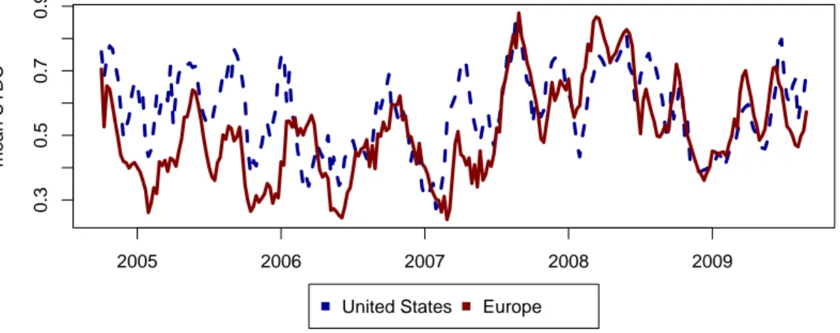
The regulatory frameworks in the US and Europe vary substantially. European banks are mostly regulated according to the Basel II framework. US banks are regulated according to rules determined by the Federal Reserve Board. A standard finding in the literature is that the regulation of European banks is more effective compared to the more fragmented regulation in the US due to shared responsibilities at the state and the federal level for the latter. Thus, European regulation is likely to coincide with lower systemic risk. Figure 2.3 depicts the evolution of upper tail dependence in the US and European banking sectors.
mean UTDC
2005 2006 2007 2008 2009
0.3 0.5 0.7 0.9
United States Europe
Figure 2.3 – Time evolution of upper tail dependence within the regional banking sectors
Upper tail dependence coefficients are estimated from a rolling time window consisting of data of the
previous 12 weeks, which is rolled across a series of daily CDS bid quotes ranging from October 2004
to October 2009 one week in each step. The above figure displays the evolution of mean upper tail
dependence, calculated as the average of all available upper tail dependence coefficients between banks
within the same region.
We observe that systemic risk in the US is mostly higher than in Europe. Especially in the first half of the sample, systemic risk is substantially lower for Europe. How- ever, at the onset of the Subprime Crisis, systemic risk increases sharply in both regions.
To test whether this relation is statistically significant, we formulate the following null hypothesis 13 :
Hypothesis 1a Systemic risk within the European banking sector is higher than within the US banking sector.
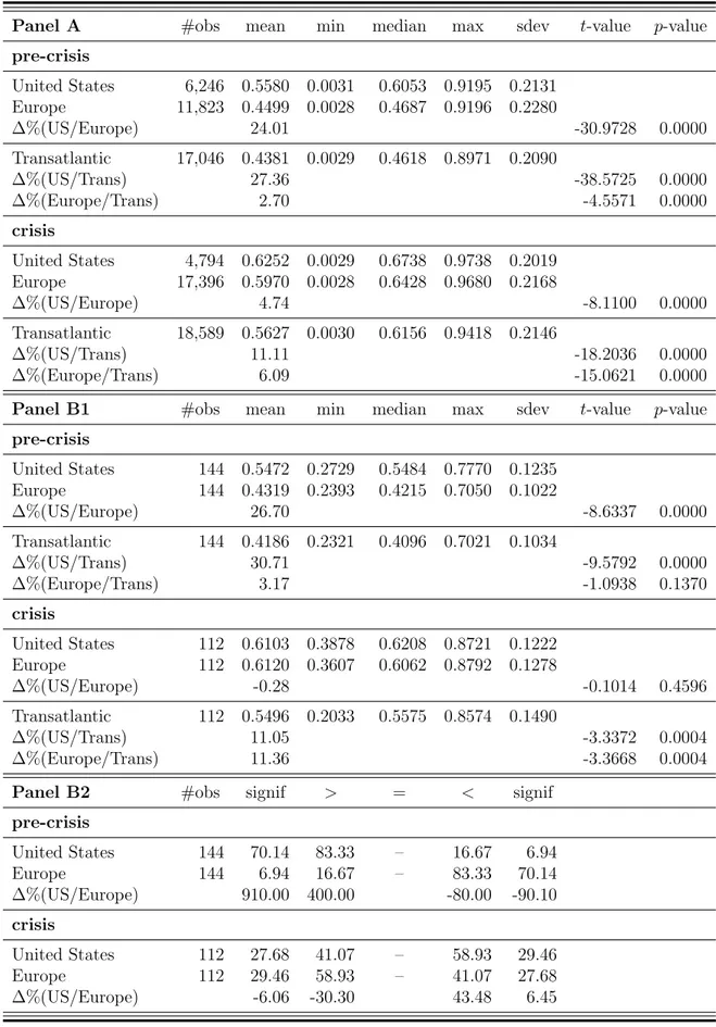
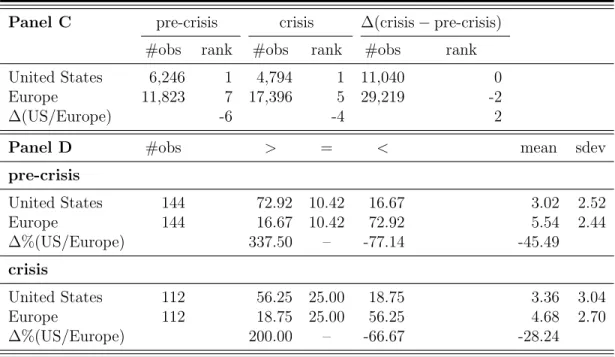
Table 2.2 presents the results of our analysis of the regional banking sectors. Panels A and B1 are organized as follows: The first column shows the region, the second column the number of observations used for the calculation of the mean, quantiles, and standard deviations in columns three to seven. The last two columns report the results of a t-test with the null hypothesis that systemic risk in Europe is higher than in the US. Statistics exhibited in Panel A are calculated according to Expression (2.5); statistics in Panel B1 are determined according to Expressions (2.7) and (2.8).
From Panel A, we observe that with a mean UTDC of 0.5872, systemic risk in the US is higher than in Europe (mean UTDC of 0.5375) by 9%. 14 This means that in the US banking sector, a bank’s probability of distress, given that another bank is in distress, is on average by 9% higher than in the European banking sector. This relation is confirmed by the values for the median UTDC (0.6362 for the US and 0.5729 for the European banking sector) as well as the aggregate figures of Panel B1, which are determined weighing all UTDC
t; I R , J R ¯
equally. Upper tail dependence in the US (0.5748) substantially exceeds upper tail dependence in Europe (0.5107). Applying t-difference tests of means reveals that the figures for the US are significantly higher than for Europe in both panels. 15 Panel B2 reports results obtained applying the count statistic from Expression (2.9).
During more than half of the observation period, systemic risk in the US is significantly higher than in Europe. In 65% of all dates t, we observe a higher mean UTDC in the US.
Approximately 80% of these upward deviations are statistically significant at the 5%-level.
13
Throughout this paper, we formulate the null hypotheses such that rejecting it confirms the economic intuition.
14
Alternatively, we compute UTDC not in a rolling window approach, but using the entire time series CDS bid premia. We find that the average UTDC estimates are higher, but that our main results still hold. The detailed figures are presented in Appendix-Table 2.7.
15