Remote sensing in coastal water monitoring:Applications in the eastern MediterraneanSea(IUPAC Technical Report)*

(1)

http://dx.doi.org/10.1351/PAC-REP-11-01-11

Remote sensing in coastal water monitoring:

Applications in the eastern Mediterranean Sea (IUPAC Technical Report)*

Manos Dassenakis

^1,‡

, Vasiliki Paraskevopoulou

¹

, Constantinos Cartalis

²

, Nektaria Adaktilou

²

, and Katerina Katsiabani

²

1Department of Chemistry, Laboratory of Environmental Chemistry, University of Athens, Panepistimioupoli Zografou, GR-15771 Athens, Greece; ²Department of Physics, Laboratory of Remote Sensing, University of Athens, Panepistimioupoli Zografou, GR-15771 Athens, Greece

Abstract: Remote sensing/satellite observation of land and oceans is a field of research that was developed during the second half of the 20^thcentury, and its importance is widely recognised because of the amount of information it can provide to the scientific community and the general public. The outcomes of remote sensing/satellite observation can be used to address and study significant aspects of environmental concern, such as habitat destruction, environmental degradation, forest fires, oil spills, and climate change. There is continuous improvement of the methods and means of remote sensing observations in order to achieve more accurate and useful information. The main advantage is the possibility of observing large areas, and the main disadvantage is that it can observe only the water and land surface.

The present paper is an effort to review the technologies used in remote sensing and the general applications in a comprehensive manner addressed to scientists who do not specialize in this area of research. Furthermore, this paper reviews case studies/applications in the Mediterranean Sea, an area affected by various polluting activities (industrial cities, agriculture, shipping, etc.) that should be continuously monitored so that the coastal countries are able to successfully manage this sensitive environment.

Keywords: chlorophyll; coastal management; eutrophication; IUPAC Chemistry and the Environment Division; Mediterranean Sea; oil spills; remote sensing.

CONTENTS

1. INTRODUCTION

2. OVERVIEW OF REMOTE SENSING TECHNOLOGY: BASIC PRINCIPLES AND SATEL- LITE CHARACTERISTICS [1]

3. REMOTE SENSING APPLICATIONS: WEATHER SATELLITES—METEOROLOGY [1]

4. REMOTE SENSING APPLICATIONS: LAND OBSERVATION SATELLITES [1]

5. REMOTE SENSING APPLICATIONS: MARINE OBSERVATION SATELLITES/SENSORS 6. REMOTE SENSING MONITORING OF OCEAN FEATURES

*Sponsoring body: IUPAC Chemistry and the Environment Division: see more details on page 373.

‡Corresponding author

(2)

7. REMOTE SENSING MONITORING OF OCEAN COLOUR (PRIMARY PRODUCTION—

CHLOROPHYLL)

8. REMOTE SENSING MONITORING OF SPM COASTAL ZONE GEOLOGICAL FEATURES 9. REMOTE SENSING MONITORING OF BIOTA

10. REMOTE SENSING MONITORING OF OIL SPILLS: SENSORS AND CASE STUDIES 11. CONCLUSIONS

MEMBERSHIP OF SPONSORING BODY REFERENCES

1. INTRODUCTION

Coastal zones are important, sensitive ecological systems and are also significant from an economic point of view as they are used for tourism, fishing, aquaculture, and recreation. Many times, their sig- nificance is ignored and they are overexploited or subjected to intense environmental pressures. Large loads of land-based pollutants from industrial, urban, and agricultural activities are disposed to coastal areas. Physical, chemical, biological, or thermal pollution can cause adverse effects to the marine environment, ecological damage, and even pose dangers to public health.

Therefore, the necessity of environmental monitoring is undisputed. There is a simultaneous need for both large-scale observation and monitoring of ocean processes as well as small-scale monitoring campaigns, e.g., for enclosed polluted gulfs, specific river catchments, etc.

Remote sensing techniques have been utilised with various types of sensors and for various applications in environmental purposes since the early 1960s. Weather monitoring and forecasting was one of the first applications of satellite remote sensing, but it was soon apparent that satellites could also be used for detailed mapping of the land surface and for the monitoring of the oceans.

The importance of marine processes in the global climate system has been stressed repeatedly, and therefore the main advantage of satellite remote sensing of the oceans is the fact that it provides large-scale and simultaneous monitoring of entire basins. At the same time, it can also be used in smaller scales and coastal areas that are subject to intense environmental pressures, but these applications have not been developed enough because of the inadequate resolution of the satellites’ sensors in small areas.

On the other hand, only a few chemical applications and/or pollutants are detectable in the marine environment by remote sensing techniques. These are chlorophyll (chl)-like pigments, suspended particulate material, and oil. In the case of oil spills, only high concentrations on the sea surface from large- scale accidents are mostly detected and monitored and not smaller accidental discharges. Therefore, there should be some effort to combine the large-scale monitoring of remote sensing with targeted in situ observations so that their results are complementary to one another with a final aim to ensure effective protection of the marine environment.

The present paper aims to review remote sensing technologies and applications. In Sections 1–5, the sensor technologies and general applications are reviewed. In Sections 6–10, there is detailed mention of remote sensing marine applications and case studies. An effort was made to focus on the Mediterranean Sea including eastern Mediterranean case studies even though there is limited work in this marine area. Large-scale case studies in the world’s oceans (Atlantic, Pacific, etc.) are beyond the scope of this paper and were not reviewed.

2. OVERVIEW OF REMOTE SENSING TECHNOLOGY: BASIC PRINCIPLES AND SATELLITE CHARACTERISTICS [1]

Remote sensing is the science of acquiring information about the Earth’s surface without actually being in contact with it. This is done by sensing and recording reflected or emitted energy and processing, analyzing, and applying that information. The process generally involves an interaction between inci-

(3)

dent radiation and the targets of interest. This is exemplified by the use of imaging systems. However, there are cases in which remote sensing also involves the sensing of emitted energy and the use of non- imaging sensors.

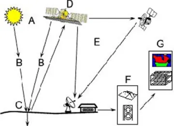
Figure 1 schematically presents the basic requirements for remote sensing applications. The energy source or illumination medium (A) provides electromagnetic energy to the target of interest. The regions of the electromagnetic spectrum mostly used for remote sensing applications are: UV (10–400 nm), visible (400–700 nm), IR (0.7–100 μm) distinguished in reflected (0.7–3μm) and thermal IR (TIR) (3–100μm), and more recently the microwave region (1 mm to 1 m). The energy travel- ing from the light source to the target and from the target to the sensors interacts with the Earth’s atmos- phere (B) and is subject to scattering and absorption. The electromagnetic spectrum regions mentioned above are not subject to significant absorption—they are called “atmospheric windows” and are thus useful for remote sensing.

The interaction between energy and target (C) depends on the properties of both the target and the radiation. There are three forms of interaction that can take place when energy strikes, or is incident upon a target surface. Absorption (A) occurs when radiation (energy) is absorbed into a target, trans- mission (T) occurs when radiation passes through it, and reflection (R) occurs when radiation

“bounces” off the target and is redirected. In remote sensing, we are most interested in measuring the radiation reflected from targets.

After the energy has been scattered by or emitted from the target, a remote sensor collects and records the electromagnetic radiation (D). Remote sensing systems, which measure energy that is naturally available, are called passive sensors. The sun provides this naturally available energy. The sun’s energy is either reflected (visible wavelengths), or absorbed and then reemitted (TIR wavelengths).

Passive sensors can only be used when the naturally occurring energy is available, which is during the day for reflected energy and both day and night for emitted energy (TIR). Active sensors, on the other hand, provide their own energy source for illumination. The sensor emits radiation, which is directed toward the target. The radiation reflected from that target is detected and measured by the sensor.

Advantages for active sensors include the ability to obtain measurements anytime, regardless of the time of day or season. Active sensors can be used for examining wavelengths that are not sufficiently provided by the sun, such as microwaves, or to better control the way a target is illuminated. However, active systems require the generation of a fairly large amount of energy to adequately illuminate targets.

Fig. 1Schematical representation of remote sensing operating principle[1], © CCRS/CCT.

(4)

Active microwave sensors are generally divided into two distinct categories: imaging and non-imaging.

The most common form of imaging active microwave sensors is RADAR. RADARis an acronym for RAdio Detection And Ranging, which essentially characterizes the function and operation of a radar sensor. The sensor transmits a microwave (radio) signal toward the target and detects the back-scattered portion of the signal. The strength of the back-scattered signal is measured to discriminate between different targets, and the time delay between the transmitted and reflected signals determines the distance (or range) to the target. Some examples of active sensors are the non-imaging altimeters and scattero - meters and the imaging SLAR (side-looking airborne radar) and SAR (synthetic aperture radar).

The energy recorded by any sensor has to be transmitted, often in electronic form, to a receiv- ing/processing station where the data are processed into an image (hard copy and/or digital) (E). The processed image is interpreted, visually and/or digitally or electronically, to extract information about the target that was illuminated (F). The final product (G) of the remote sensing process is achieved when we apply the information we have been able to extract from the imagery about the target in order to better understand it, reveal some new information, or assist in solving a particular problem.

Although ground-based and aircraft platforms may also be used, satellites provide most of the remote sensing imagery used today. Satellites have several unique characteristics, which make them particularly useful for remote sensing of the Earth’s surface. The main satellite characteristics are discussed below.

The path followed by a satellite is referred to as its orbit. Satellite orbits are matched to the capability and objective of the sensor(s) they carry. Orbit selection can vary in terms of altitude (their height above the Earth’s surface) and their orientation and rotation relative to the Earth. The geostationary satellites rotate with the Earth continuously over a specific area, like the satellites used for weather applications and communications. Other satellites follow near-polar orbits, which means that they are ascending toward the North Pole and then descend toward the South Pole, thus achieving full coverage of the Earth’s surface due to its rotation.

The spatial resolutionof the sensor determines the detail discernible in an image and refers to the size of the smallest possible feature that can be detected. The area on the ground “seen” by a satellite is called the resolution cell and determines a sensor’s maximum spatial resolution.

Most remote sensing images are composed of a matrix of picture elements, or pixels, which are the smallest units of an image. Image pixels are normally square and represent a certain area on an image. If a sensor has a spatial resolution of 20 m and an image from that sensor is displayed at full resolution, each pixel represents an area of 20 ×20 m on the ground. In this case, the pixel size and resolution are the same. However, it is possible to display an image with a pixel size different than the resolution.

Spectral resolutiondescribes the ability of a sensor to define fine wavelength intervals. The finer the spectral resolution, the narrower the wavelength range is for a particular channel or band. Many remote sensing systems record energy over several separate wavelength ranges at various spectral resolutions. These are referred to as multispectral sensors. Advanced multispectral sensors, called hyperspectral sensors, detect hundreds of very narrow spectral bands throughout the visible, near-IR, and mid-IR portions of the electromagnetic spectrum. Their very high spectral resolution facilitates fine discrimination between different targets based on their spectral response in each of the narrow bands.

The radiometric resolutionof an imaging system describes its ability to discriminate very slight differences in energy. The finer the radiometric resolution of a sensor, the more sensitive it is to detecting small differences in reflected or emitted energy.

In addition to spatial, spectral, and radiometric resolution, the concept of temporal resolutionis also important. The revisit period refers to the length of time it takes for a satellite to complete one entire orbit cycle. The revisit period of a satellite sensor is usually several days. Therefore, the absolute temporal resolution of a remote sensing system to image the exact same area at the same viewing angle a second time is equal to this period. However, because of some degree of overlap in the imaging swaths of adjacent orbits for most satellites and the increase in this overlap with increasing latitude, some areas

(5)

of the Earth tend to be re-imaged more frequently. Also, some satellite systems are able to point their sensors to image the same area between different satellite passes separated by periods from one to five days. Thus, the actual temporal resolution of a sensor depends on a variety of factors, including the satellite/sensor capabilities, the swath overlap, and latitude. The ability to collect imagery of the same area of the Earth’s surface at different periods of time is one of the most important elements for applying remote sensing data.

3. REMOTE SENSING APPLICATIONS: WEATHER SATELLITES—METEOROLOGY [1]

Weather monitoring and forecasting was one of the first civilian (as opposed to military) applications of satellite remote sensing. Today, several countries operate weather, or meteorological, satellites to monitor weather conditions around the globe. Generally speaking, these satellites use sensors that have fairly coarse spatial resolution (when compared to systems for observing land) and provide large areal coverage. Their temporal resolutions are quite high, providing frequent observations of the Earth’s surface, atmospheric moisture, and cloud cover, which allows for near-continuous monitoring of global weather conditions, and hence, forecasting. Some satellites used for weather applications since the 1960s were the following:

• NASA (U.S. National Aeronautics and Space Administration) in collaboration with NOAA (U.S.

National Oceanic and Atmospheric Administration) launched the ATS series (Applications Technology Satellites) and later the GOES (Geostationary Operational Environmental System) which are geostationary satellites covering one third of the Earth, namely, North and South America, the Pacific Ocean, and most of the Atlantic Ocean. The sensors of these satellites operate in the vis/IR parts of the electromagnetic spectrum and they detect cloud, pollution, haze, storms, fog, ice clouds, forest fires, volcanoes, moisture, rain fall, and sea surface temperature (SST).

• Another NASA-NOAA satellite series are the AVHRR (Advanced Very High Resolution Radiometer) satellites with near-polar orbits providing global coverage of cloud, snow, ice, water, vegetation, SST, volcanoes, forest fires, and moisture with observations in the vis/IR and TIR spectrum.

• Some more weather satellites are operated by the United States and the DMSP (Defense Meteorological Satellite Program). These are near-polar orbiting satellites with two broad wavelength bands (visible to near-IR and TIR band). An interesting feature of the sensor is its ability to acquire visible band night-time imagery under very low illumination conditions, and thus it can acquire striking images of the Earth showing the night-time lights of large urban centres.

• There are several other meteorological satellites in orbit, launched and operated by other countries, or groups of countries. These include Japan, with the GMS satellite series, and the consor- tium of European communities, with the Meteosat satellites. Both are geostationary satellites sit- uated above the Equator over Japan and Europe, respectively.

4. REMOTE SENSING APPLICATIONS: LAND OBSERVATION SATELLITES [1]

Although many of the weather satellite systems (such as those described in the previous section) are also used for monitoring the Earth’s surface, they are not optimized for detailed mapping of the land surface. NASA and NOAA operated since 1972 the Landsat series of satellites which later became com- mercialised and provide data to civilian and applications users. The orbits are near-polar, and the sensors multispectral scanner (MSS) and thematic mapper (TM) operating in the vis/IR and TIR spectrum can record images and provide information on soil-vegetation, altimetry, mineral rock types, cultural features and moisture that can be used for resource management, cultural and thermal mapping, environmental monitoring, and detection of change (e.g., monitoring forest clear-cutting).

(6)

SPOT (Système Pour l’Observation de la Terre) is a series of Earth observation imaging satellites designed and launched by CNES (Centre National d’Études Spatiales) of France, with support from Sweden and Belgium. The HRV (high resolution visible) sensors of SPOT allow applications requiring fine spatial detail (such as urban mapping) to be addressed. Furthermore, SPOT is useful for applications that require frequent monitoring, e.g., agriculture and forestry.

The Indian Remote Sensing (IRS) satellite series combines features from both the Landsat MSS/TM sensors and the SPOT HRV sensor, thus providing high-resolution data useful for urban planning, mapping applications, vegetation discrimination, and natural resource planning.

Currently, there are several satellites used for land observation purposes launched by national space agencies (e.g., United States, Canada, China, Japan, Italy, Brazil, Germany, etc.) as well as regional or international agencies (European Space Agency, ESA) [2].

The usefulness of satellite remote sensing for land monitoring applicationscan be summarised as follows. Satellite and airborne images are used as mapping tools to monitor crop type, health, yield estimation, soil characteristics, soil management, and farming practices. Multispectral sensors (UV to IR) provide information on the phenology (growth), stage type, and crop health; radar is sensitive to the structure, alignment, and moisture content of the crop and thus can provide complementary information to the optical data. Images of crops can be obtained throughout the growing season to not only detect problems, but also to monitor the success of the treatment.

Forestry applicationsof remote sensing include reconnaissance mapping (forest cover updating and measuring biophysical properties of forest stands), forest cover-type discrimination, commercial forestry inventory and mapping applications for companies and resource management agencies, and, finally, environmental monitoring for conservation authorities, which refers to information on defor- estation (rainforest, mangrove colonies), species inventory, watershed protection, coastal protection (mangrove forests), and forest health. Large-scale species identification can be performed with multispectral, hyperspectral, or air-photo data, while small-scale cover-type delineation can be performed by radar or multispectral data interpretation. Remote sensing can be used to detect and monitor forest fires and the regrowth following a fire. NOAA AVHRR thermal data and GOES meteorological data can be used to delineate active fires and remaining “hot spots” when optical sensors (photo–video) are hin- dered by smoke, haze, and/or darkness.

Geological applications of remote sensing include: surficial deposit/bedrock, lithological and structural mapping, sand and gravel (aggregate) exploration/exploitation, mineral exploration, hydro- carbon exploration, environmental geology, geobotany, sedimentation mapping and monitoring, event mapping and monitoring, geohazard mapping, and planetary mapping. Multispectral data can provide information on lithology or rock composition based on spectral reflectance. Radar provides an expres- sion of surface topography and roughness, and thus is extremely valuable, especially when integrated with another data source to provide detailed relief. Remote sensing gives the overview required to (1) construct regional unit maps, useful for small-scale analyses, and planning field traverses to sample and verify various units for detailed mapping; and (2) understand the spatial distribution and surface relationships between the geological units.

Examples of hydrological applicationsinclude wetlands mapping and monitoring, soil moisture estimation, snow pack monitoring/delineation of extent, measuring snow thickness, determining snow- water equivalent, river and lake ice monitoring, flood mapping and monitoring, glacier dynamics monitoring (surges, ablation), river/delta change detection, drainage basin mapping and watershed modeling, irrigation canal leakage detection, and irrigation scheduling. Passive and active radar sensors have brought a new dimension to hydrological studies with its active sensing capabilities, allowing the time window of image acquisition to include inclement weather conditions or seasonal or diurnal darkness.

Also, coarse resolution optical sensors such as NOAA’s AVHRR are used to provide an excellent overview of pack ice extent if atmospheric conditions are optimal (resolution = 1 km).

Land use applicationsof remote sensing include the following: natural resource management, wildlife habitat protection, baseline mapping for geographical information system (GIS) input, urban

(7)

expansion/encroachment, routing and logistics planning for seismic/exploration/resource extraction activities, damage delineation (tornadoes, flooding, volcanic, seismic, fire), legal boundaries for tax and property evaluation, and target detection/identification of landing strips, roads, clearings, bridges, and land/water interface [1].

The main mapping applications of remote sensing are: (a) planimetry (identification and geo - location of basic land cover, e.g., forest, marsh, drainage, and anthropogenic features, e.g., urban infrastructure, transportation networks in the x, yplane with the provided information to be used for large- scale applications such as surban mapping, facilities management, military reconnaissance, and general landscape information); (b) digital elevation models (DEMs); and (c) baseline thematic mapping/topographic mapping. Finally, there is a growing demand for digital databases of topographic and thematic information to facilitate data integration and efficient updating of other spatially oriented data.

All of the above applications are combined with GIS.

5. REMOTE SENSING APPLICATIONS: MARINE OBSERVATION SATELLITES/SENSORS

The Earth’s oceans cover more than two-thirds of the Earth’s surface and play an important role in the global climate system. They also contain an abundance of living organisms and natural resources that are susceptible to pollution and other man-induced hazards. The meteorological and land observation satellites/sensors that have already been discussed in Section 3 can also be used for monitoring the oceans, but there are other satellite/sensor systems that have been designed specifically for this purpose [1].

The Nimbus-7 satellite, launched in 1978 and placed in a sun-synchronous, near-polar orbit, carried the first sensor, the coastal zone colour scanner (CZCS), specifically intended for monitoring the Earth’s oceans and water bodies. The primary objective of this sensor was to observe ocean colour and temperature, particularly in coastal zones, with sufficient spatial and spectral resolution to detect pollutants in the upper levels of the ocean and to determine the nature of materials suspended in the water column. The repeat cycle of the satellite allowed for global coverage every six days. The CZCS sensor consisted of six spectral bands in the visible, near-IR, and thermal portions of the spectrum. Bands 1 to 4 of the CZCS sensor (0.43–0.68 μm) were very narrow and optimized to allow detailed discrimination of differences in water reflectance owing to phytoplankton concentrations and other suspended partic- ulates in the water. In addition to detecting surface vegetation on the water, band 5 was used to discriminate water from land prior to processing the other bands of information, and finally band 6 was used for monitoring SST. The CZCS sensor ceased operation in 1986 [1].

The first marine observation satellite (MOS-1) was launched by Japan in February 1987 and was followed by its successor, MOS-1b, in February 1990. These satellites carried three different sensors: a four-channel multispectral electronic self-scanning radiometer (MESSR), a four-channel visible and thermal infrared radiometer (VTIR), and a two-channel microwave scanning radiometer (MSR). The MESSR bands are quite similar in spectral range to the Landsat MSS sensor and are thus useful for land applications in addition to observations of marine environments [1].

The SeaWiFS (sea-viewing wide field-of-view sensor) on board the SeaStar spacecraft is an advanced sensor designed for ocean monitoring. It consists of eight spectral bands of very narrow wavelength ranges tailored for very specific detection and monitoring of various ocean phenomena including: ocean primary production and phytoplankton processes, ocean influences on climate processes (heat storage and aerosol formation), and monitoring of the cycles of carbon, sulfur, and nitrogen [1].

A limitation to the exploitation of SeaWiFS is that the instrument is operated as a commercial venture with research use purchased by NASA. Operational and some near-real-time applications cannot be supported through NASA and data must be purchased from Orbview (Orbital Sciences Corporation) [3].

The first of a next generation of ocean colour instruments, the moderate resolution imaging spectro radiometer (MODIS), was launched on 18 December 1999 on-board the NASA “Terra” satellite.

(8)

MODIS represents a further leap in capability compared to SeaWiFS with more wavebands, higher signal-to-noise ratio, more complex on-board calibration, and the capability of simultaneous observation of ocean colour and SST. Further instrument launches were planned, including MODIS on “Aqua” platform (2002). This will ensure continuity of ocean colour data, and will provide two observations per day (because Terra and Aqua will pass overhead at 10:30 and 14:30 h local time, respectively). MODIS broadcasts continuously, signals can be recorded by anyone with an appropriate receiver and therefore can be used without any commercial restrictions [3,4].

The MERIS imaging multispectral radiometer (vis/IR) was launched on ESA’s Envisat platform in 2002. Its main objective is to monitor ocean colour, but atmospheric and land applications are also carried out [5–7].

The NASA Aquarius project is a focused satellite mission to measure global sea surface salinity.

After its planned 2010 launch, it will provide the global view of salinity variability needed for climate studies. The objectives of this mission are to produce global salinity maps at 0.2 psu accuracy on a monthly basis at 100-km resolution (1 psu = 1 gⴢkg^–1salt concentration in seawater) and measure the seasonal and year-to-year variations of salinity, as well as the global annual mean [8].

The ocean-observing systems/sensors mentioned in the above sections are important for global and regional-scale monitoring of ocean pollution and health, and assist scientists in understanding the influence and impact of the oceans on the global climate system. In the following sections, there will be mention of oceans and coastal applications, the necessary validation and comparison of remote sensing to in situ data and specific case studies with focus on the Mediterranean Sea.

6. REMOTE SENSING MONITORING OF OCEAN FEATURES

Satellite thermal images, such as those obtained by AVHRR-SST have been used in order to define the time and space scales of surface temperature distributions. Apart from the use of SST data to assess climate change, the temperature distributions are related to the upper thermocline circulation. For this purpose, the satellite images are compared with conductivity–temperature–depth (CTD) casts and acoustic Doppler current profiler (ADCP) measurements during oceanographic cruises. The objectives of this integrated analysis are to provide knowledge on basin-scale circulation as well as to monitor phenomena of smaller scales, such as eddies and local currents [9–14]. Furthermore, altimeter satellite data (ERS) have been compared with buoy observations to determine not only water circulation but also sea- level statistics [15]. Some recent applications of remote sensing data in physical oceanography in the Mediterranean and Black Sea basins will be briefly presented.

An SST study of the Black Sea was carried out in order to investigate seasonal and interannual variability during the period from November 1981 to December 2000. Night-time weekly multichannel sea surface temperature (MCSST) data set based on NOAA AVHRR measurements (with spatial and temperature resolution of about 18 km and 0.1 °C) were used. The SST satellite fields averaged for the central months of four hydrological seasons (February, May, August, and November) were calculated and compared with the corresponding climatic SST fields based on in situ measurements. It turned out that the winter weekly mean SST minima fell on 1985, 1987, 1992, and 1993, SST maxima on 1984, 1988, 1995, and 1999. Since 1994, winters were relatively warm. Most of the marked anomalies of the summer and winter SSTs as well as the greatest seasonal amplitudes of SST (in 1987, 1992, and 1998) occurred either during the El Niño global events or some months later. An increasing trend of the Black Sea mean SST of about 0.09 °C per year over the period of consideration was revealed, the western deep-sea region getting warmer more slowly (about 0.08 °C per year) as compared with the eastern one (about 0.11 °C per year). In the first half of the period (1982–1991), the trends of the yearly and sea- sonally mean (besides the summer-averaged) SSTs were considerably less than in the second one (1992–2000); the summer-averaged SST trend was approximately the same in both of the subperiods [9].

(9)

A 10-year data set of AVHRR-SST with 18-km space resolution and weekly frequency was used to study the seasonal and inter-annual variability of the eastern Mediterranean Sea surface field. Three main objectives were addressed. The first was to define the time and space scales of the surface temperature distributions. The second objective was to relate the SST features to the upper thermocline circulation, and the third was to compare these features with the observational evidence of the Physical Oceanography of the Eastern Mediterranean (POEM) Program [10,11].

The time analysis revealed the presence of a strong seasonal signal characterized by two main seasonal extremes, winter and summer. The space analysis shows that the dominant scale is the sub-basin scale and the sub-basin gyres are very well resolved, allowing the identification of permanent and semi- permanent structures. The results for the two further objectives can be summarized together. The seasonal and monthly SST distributions are strongly correlated with the dynamical structure of the basin upper thermocline circulation. A direct comparison of the September 1987 SST pattern with the corresponding surface temperature map of the POEM-87 survey proves this correlation quantitatively.

Furthermore, comparison of the SST monthly climatologies with the POEM circulation scheme showed that all the major currents and the sub-basin gyres were also found consistent with the patterns dictated by the remote sensing data (Fig. 2) [10,11].

A study of satellite and in situ data for the eastern basin of the Mediterranean Sea was undertaken in order to verify the historically proposed Atlantic water (AW) circulation schemes. The study included detailed analysis of over 1000 daily and weekly composite images spanning the period 1996–2000, and of monthly composite images available since 1985. Whenever in situ observations were available, they were compared with the satellite thermal signatures and it was shown that both were consistent. The results of this study confirmed that AW circulates counterclockwise in the eastern basin. However, the Fig. 2SST field of September 1987. Left: POEM data above, AVHRR data below. Right: correlation of the two data sets (adapted from ref. [10]).

(10)

historical schemes represent a broad flow while this study showed that the circulation is essentially con- strained along slope, being markedly unstable and generating mesoscale eddies (Fig. 3) [12].

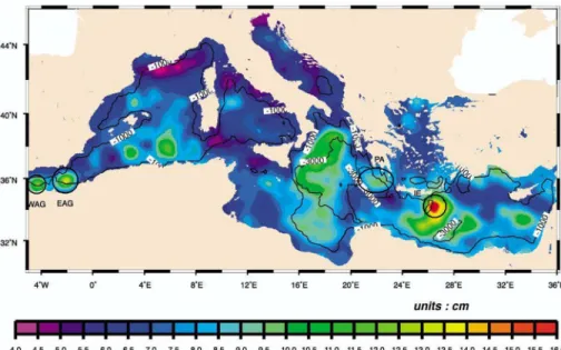
In another study, seven years of combined maps of TOPEX/Poseidon (T/P) and ERS-1/2 alti meter data were used to describe the surface circulation variability in the Mediterranean Sea. The longer study period (1993–1999) and the merging of T/P and ERS-1/2 altimeter data allowed observation with a good accuracy the major changes that occurred in the Mediterranean Sea and, in particular, at basin and sub-basin scales. First, important interannual signals were found in the Ionian basin where the cyclonic circulation has clearly intensified since 1997. In the Levantine basin, although the Ierapetra eddy exhibits a clear seasonal cycle, it is not always present during the observation period. Secondly, the seasonal cycle of the Alboran gyres was confirmed. Moreover, these gyres and the Ierapetra eddy consti- tute the most intense signals of the Mediterranean Sea variability (Fig. 4). Finally, this descriptive study illustrated the need to continue monitoring the surface circulation in order to better understand the dynamics of the Mediterranean Sea [13].

Fig. 3 The eastern basin of the Mediterranean Sea in January 1998 (SST, a), and the remote sensing surface circulation scheme (b) [12].

(11)

Through the analysis of satellite thermal images, mesoscale anticyclonic eddies have been observed to recurrently drift along the northwestern Mediterranean coasts and the Algerian basin [14–16]. In one case, a group of anticyclonic structures were tracked from the Gulf of Lions to the Catalan shelf by analysis of SST images, and at the same time one of the eddy-like features was also intensely surveyed by means of in situ CTD casts and repeated fast surveys with oscillating CTD and ADCP measurements. It was found that the passage of the eddy modified the local flow, involving advection and subduction of surrounding waters (Fig. 5) [16].

Fig. 4The variability of SLA from combined maps of T/P and ERS-1/2 (1993–1999). Units are in cm. WA/EAG:

western/eastern Alboran gyres; PE: Pelops anticyclone, IE: Ierapetra eddy [13].

Fig. 5SST image of 26 September. The ADCP velocity field is superimposed to the satellite image [16].

(12)

7. REMOTE SENSING MONITORING OF OCEAN COLOUR (PRIMARY PRODUCTION—CHLOROPHYLL)

The term “ocean colour” is used to indicate the visible light spectrum as observed at the sea surface, which is related, by the processes of absorption and scattering, to the concentration of water constituents, specifically chl-like pigments from phytoplankton (microscopic unicelluar algae) as well as suspended sediments, degrading organic materials, and other particulate or dissolved substances. The retrieval of environmental parameters depends on modeling the relationship between water optical properties and concentration of water constituents [17]. In this section, the quantification of oceanic phytoplankton (primary production) through satellite remote sensing of sea surface colour will be discussed in detail.

Remote sensing measurements of sea surface colour and temperature, as mentioned above, have been historically conducted by means of low-resolution (pixels of the order of 1 km) data collected in the vis/IR and TIR spectral region. Optical remote sensing allows monitoring the space and time hetero - geneity of phytoplankton growth in marginal and enclosed seas, a factor critical to understanding their ecosystem dynamics [17,18].

Studies concerning sea surface optical properties relied primarily on historical data generated by CZCS, which was launched in the fall of 1978. The available data from CZCS, even though they were characterized by limited statistical coverage (owing to the low number and irregular time spacing of individual images), show consistent patterns in line with the characteristics of the European basins. In general, the same kind of large-scale colour patterns were recurrent on a regional and seasonal basis, in different years [17].

In the Mediterranean region, in particular, the ocean colour data provide indications on a number of processes owing to biological, geochemical, and physical interactions—in particular, those related to the environmental impact of coastal and river runoff, coupled with water circulation patterns. The quasi- permanent surface features of the basin are exemplified in the composite CZCS image of Fig. 6, which shows the mean annual patterns of water constituents for the period 1979–1985. The original data (2373 individual images) were processed to derive chl-like pigment concentration. The basin presents

Fig. 6 Composite CZCS image of the Mediterranean basin. This image highlights the differences between Mediterranean sub-basins, the oligotrophic waters of the open sea, and the mesotrophic waters of coastal areas [17].

(13)

relatively clear, oligotrophic waters in the pelagic region, where the signal, owing to planktonic pigments, is minimum. Oligotrophic conditions are most persistent, over the annual cycle, in the eastern rather than in the western Mediterranean. Accordingly, seasonal variations were most pronounced in the western rather than in the eastern Mediterranean [17].

On the other hand, the basin presents highly dynamic, mesotrophic, at times even eutrophic, sub- basins and near-coastal areas. Not surprisingly, therefore, the Mediterranean CZCS data set suggests several points of particular interest for the study of the coastal domain. Major rivers such as the Po, Rhone, Ebro (and the Nile, up to a point) or the Danube, Dnestr, and Dnepr in the Black Sea area, have distinct plumes interacting with the marine environment. Within the range of the plumes (as with coastal runoff in general), it is often impossible for the CZCS to distinguish the signature of biogenic pigments from that of the total load of dissolved and suspended materials present in the water. However, the observation of such features provides important clues on coastal frontal dynamics and potential correlations with nutrient enrichment, sediment transport, and pollution sources. An example of coastal interactions because of fluvial runoff in the northern Adriatic Sea is shown in the CZCS image of Fig. 7.

Note the plume originated by the Po River (4 July 1980). The environmental characteristics of the Gulf of Venice appear to be dominated by waters of fluvial origin [17].

In Fig. 8, the Nile River plume is shown instead, as it appeared to the CZCS on 25 November 1981. The coastal black rim highlights shallow waters with very high sediment load. The western portion of the plume is seen interacting with coastal currents. The connection between the eastern portion of the plume and a series of coastal filaments can be seen. In the land portion, the vegetated area of the Nile River delta, and in part the major branches of the river itself, are marked by darker tones [17].

Fig. 7Coastal features due to coastal and fluvial runoff in the northern Adriatic Sea [17].

(14)

Similar Black Sea data dated 28 June 1979, shown in Fig. 9, illustrate the effect of massive river discharges in the coastal zone of an enclosed basin. The main feature of the whole Black Sea is in fact the high pigment concentration, possibly related to the combined effect of fluvial runoff, strong vertical stratification, and circulation features in general, on the presence and abundance of suspended and dissolved matter in surface waters. The extent of the impact of river discharges along the western coast (i.e., both a direct one owing to the sediment load and one induced on the planktonic flora by the nutrient load), from the Danube delta in particular, on the Black Sea surface colour field can be readily evaluated. The features traced by high pigments along the southern coast appear to be entrained in the interacting cyclonic circulations of the western and eastern sub-basins. Small plumes of high-pigment waters extending from the Bosphorus also seem to trace the Black Sea outflow into the Sea of Marmara (Fig. 9) [17].

The list of sensors that became available after CZCS for coastal/marine observations in the optical range, included the SeaSeaWIFS, in 1996; the ocean colour and temperature scanner (OCTS), also in 1996; the medium resolution imaging spectrometer (MERIS), and possibly follow-ups in the ERS family, in 1998; and the Earth observing system (EOS) suite of sensors, planned in the late 1990s as well, to name just a few [17].

The next tool that provided the ocean bio-geochemical remote sensing community with significant data was the SeaWiFS. The SeaWiFS Project Office was formally initiated by NASA in 1990. The sensor was finally launched by the Orbital Sciences Corporation in 1996 to provide five years of science-quality data for global ocean bio-geochemistry research. To date, the SeaWiFS program has greatly exceeded the mission goals established when it was launched in terms of data quality, data accessibility and usability, ocean community infrastructure development, cost efficiency, and community service. The SeaWiFS Project Office and its collaborators in the scientific community have made substantial contributions in the areas of satellite calibration, product validation, near-real-time data access, field data collection, protocol development, in situ instrumentation technology, operational data system development, and desktop level-0 to level-3 processing software [19].

Fig. 8The Nile River plume (CZCS image, 25 November 1981) [17].

(15)

The riginal SeaWiFS program goals and project objectives were as follows:

• to determine the spatial and temporal distributions of phytoplankton blooms, along with the mag- nitude and variability of primary production by marine phytoplankton on a global scale,

• to quantify the ocean’s role in the global carbon cycle and other bio-geochemical cycles,

• to identify and quantify the relationships between ocean physics and large-scale patterns of pro- ductivity,

• to understand the fate of fluvial nutrients and their possible effects on carbon budgets,

• to identify the large-scale distribution and timing of spring blooms in the global oceans,

• to acquire global data on marine optical properties, along with a better understanding of the processes associated with mixing along the edge of eddies and boundary currents, and

• to advance the scientific applications of ocean-colour data and the technical capabilities required for data processing, management, and analysis in preparation for future missions [19].

The quality of the data products of SeaWIFS was evaluated primarily on the comparisons with in situ data. For chlorophyll-a (chl-a), the slope and r²were 1.00 and 0.892 and 1.03 and 0.85, for 2804 match-ups and 262 match-ups, respectively, over a range of 0.03 to around 90 mg m^–3(Figs. 10a,b).

The in situ data of Fig. 10a included only 113 cases from the Sargasso Sea and 35 cases from the North Adriatic (Mediterranean region) [19–21].

Standard SeaWIFS algorithms have been demonstrated to be inappropriate over the Mediterranean region. Therefore, in some papers uncertainties in the retrieval of satellite surface chl concentrations in the Mediterranean Sea have been evaluated using both regional and global (SeaWIFS) Fig. 9Black Sea surface colour field (CZCS image, 28 June 1979) [17].

(16)

ocean colour algorithms. The rationale for this effort was to define the most suitable ocean colour algorithm for the reprocessing of the entire SeaWiFS archive of the Mediterranean [22,23].

In one case, using a large dataset of coincident in situ chl and optical measurements, covering most of the trophic regimes of the Mediterranean basin, two existing regional algorithms and the global algorithm OC4v4 used for standard NASA SeaWiFS products were validated. The results of the analysis confirmed that the OC4v4 performs worse than the two existing regional algorithms, leading to a significant overestimation of the SeaWiFS-derived chl concentration (>70 % for chl <0.2 mgⴢm^–3). The two regional algorithms also showed uncertainties dependent on chl values. Then, a better tuned algorithm was introduced, the MedOC4. The results confirmed that MedOC4 is the best algorithm match- ing the requirement of unbiased satellite chl estimates and improving the percentage of the satellite uncertainty, and that the NASA standard chl products are affected by an uncertainty of the order of 100 %. Moreover, the analysis suggests that the poor quality of the SeaWiFS chl in the Mediterranean is not due to the atmospheric correction term but to peculiarities in the optical properties of the water column. Finally, the observed discrepancy between the global and the regional bio-optical algorithms has been discussed. The main result was the inherent bio-optical properties of the basin can explain the observed discrepancy. In particular, the oligotrophic water of the Mediterranean Sea is less blue (30 %) and greener (15 %) than the global ocean. Possible explanations for this are attributed to a proposed different phytoplankton community, structure and distributions in the Mediterranean, such as the presence of coccolitophores, the dominance of prokaryots, or a high ratio among eterotrophs and autotrophs [22].

In another research case (eastern Mediterranean, Cyprus eddy) the standard SeaWiFS OC4v4 algorithm generated data and MODIS chlor_a2 algorithm data overestimated chl-a as previously reported, while a regional algorithm proposed by Bricaud et al. 2002 [24] and the semi-analytical MODIS chlor_a3 algorithm gave improved retrievals (Fig. 11) [23].

SeaWiFS-derived (1998–2003) data were used to monitor algal blooming patterns and anomalies in the Mediterranean basin. Yearly and monthly means of chl-like pigment concentration were com- puted for these six years, and climatological means were derived (Fig. 12). The space and time patterns of the chl field appear to concur with the Mediterranean general oceanographic climate, while the chl anomalies describe trends and “hot spots” of algal blooming [18].

The analysis showed a general decrease of chl values in the yearly and monthly means and an ear- lier anticipation of the northwestern spring bloom, in comparison to what was seen in historical CZCS (1979–1985) data. These have been interpreted as symptoms of an increased nutrient limitation, resulting from reduced vertical mixing owing to a more stable stratification of the basin, in line with the gen- Fig. 10Comparison of in situ and satellite chl a values: (a) algorithm OC4v4 data compared with in situ data 2804 match-ups [21], (b) algorithm OC4v4 data compared with in situ data 262 match-ups, fourth reprocessing of satellite data including all available improvements used by the SeaWifs Project Office [19].

(17)

eral warming trend of the Mediterranean Sea in the last 25 years. At the same time, the recurrent increasing blooms at the various hot spots have been described as localized phenomena, linked to either air–sea interactions in pelagic domain (Lion and Rhodes gyres), or increased nutrient availability and low water renewal in coastal areas. The latter kind of anomalous blooms would be related to the anthropogenic impact on coastal sites (e.g., crowded beaches or marinas) or to the combination of specific geographical and meteorological conditions (e.g., enclosed bays during summer, when hydrodynamic Fig. 11SeaWiFS and MODIS retrievals compared to in situ data with different algorithms [23].

Fig. 12SeaWiFS-derived (1998–2003) climatological chl yearly mean, Mediterranean Sea [18].

(18)

forcing is low). This would suggest that noxious, or harmful, blooms (known to have occurred in the areas and periods considered) are predominantly local phenomena, with little or no connection to regional events [18].

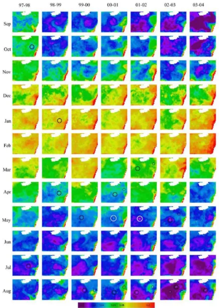
In a study of the cycling of phosphorus in the Mediterranean, the (CYCLOPS) research team investigated phosphate limitation in the eastern Mediterranean at the centre of an anticyclonic eddy south of Cyprus. SeaWiFS mean chl-a maps were presented for the eastern Mediterranean for each month between September 1997 and August 2004. These maps (Fig. 13) showed that chl-a in the region decreased over the duration of the time series with reductions in the centre of the eddy, tracked using a quasi-Lagrangian approach, of approximately 33 % between 1997 and 1998 and 2002 and 2003. It was hypothesized that the variations in chl-a were partly a function of the eddy dynamics [23].

Fig. 13Individual monthly chl-a maps using the B2002 algorithms with overlaid eddy centre locations determined from in situ observations: large black circle, “main” Cyprus eddy; small black circle, “secondary” eddies; large white circle, CYCLOPS cruises in May 2001 and 2002 [23].

(19)

In some cases, satellite remote sensing has been used to assess water quality in smaller scales, for example, particular coastal areas. Such an effort was the use of Landsat 7 ETM+ data in order to assess water quality in the coastal area of Tripoli (Lebanon) and provide a first baseline for coastal resources management. In situ data, collected in the field within 6 h before/after the time of the satellite overpass, were used to derive empirical algorithms for chl-a concentration, Secchi disk depth, and turbidity. Then, maps of the distribution of the selected water quality parameters were generated for the entire area of interest, and compared with analogous results obtained from SeaWiFS data. The maps indicate that the Tripoli coastal area is exposed to moderate eutrophic conditions along most of its shoreline (in particular, along the northern stretch), in correspondence with fluvial and wastewater runoff sources. The Landsat 7 ETM+ data proved useful for the intended application, and will be used to start a national database on water quality in the Lebanese coastal environment [25].

Another such effort to combine satellite and in situ monitoring was carried out by Greek researchers. The research was applied for the eastern coastal area of Lesvos Island. The concentration of chl-a, water transparency, and SST were measured in situ at the date and time of satellite overpass (Fig. 14). The aim of the study was to assess the ability to determine the above-mentioned parameters by Landsat-TM satellite images [26].

Finally, in the case of local water quality monitoring of coastal areas a similar approach has been to use aircraft-carried sensors. In such a research activity, the hyperspectral compact airborne spectro- graphic imager (CASI) sensor was implemented to monitor water quality in a transitional zone from polluted to clean sea-water, in Haifa Bay and adjacent river estuaries, at the northern part of the Mediterranean coast of Israel. Synoptic measurements of optical data acquired from the airborne scanner were used to map chl-a and suspended particulate matter (SPM) concentrations in surface waters in the study area (Fig. 15). This airborne hyperspectral scanner was found to be an expedient monitoring tool for the relatively small geographic area of the current study, as it was able to reveal the patchy distribution and sharp concentration changes of the mapped water characteristics. The chl-a concentrations mapped and measured in this survey were unusually low (<2 μgⴢdm^–3) owing to a long-period inter- mission of anthropogenic phosphate and nitrate input to the bay. The SPM and chl-a spatial distribution Fig. 14Landsat-TM satellite images of chl-a in Lesbos straits (Greece) [26].

(20)

along the lower river system exhibit variations which could be plausibly explained by the hydrological structure and geochemical impacts on the riverine water sources [27].

One of the latest and most advanced applications of remote sensing ocean colour is the distribution of phytoplankton to size types or classes from satellite data. Until recently, the principal goal of satellite-borne sensing of ocean colour was to create synoptic fields of phytoplankton biomass (as chl-a concentration). In the context of climate change, a major application has been the modeling of primary production and the ocean carbon cycle. It is now recognised that a partition of the marine autotrophic pool into a suite of phytoplankton functional types (PFTs), each type having a characteristic role in the bio-geochemical cycle of the ocean, would increase our understanding of the role of phytoplankton in the global carbon cycle. At the same time, new methods have been emerging that use visible spectral radiometry to map some of the PFTs. Attempts to identify PFTs from space represent a new development, with potential for further improvement, owing to the increasing improvement in both spectral and radiometric resolution of satellite sensors as well as the understanding of phyto plankton optical properties. But it is just as important to realise that remote sensing cannot provide all the answers. What is needed is a judicious combination of in situ and remote sensing techniques, to help extract maximum information on the distribution of PFTs at the global scale [28].

A model has been developed that is able to link phytoplankton absorption to phytoplankton size classes (PSCs). This model uses the optical absorption by phytoplankton at 443 nm, symbolized aph(443), which can be derived from the inversion of ocean colour data. The model is based on the observation that the absolute value of aph(443) co-varies with the spectral slope of phytoplankton absorption in the range of 443–510 nm, which is also a characteristic of PSCs. The model, used for SeaWiFS global data, showed that picoplankton (0.2–2 μm) dominated in surface waters (~79.1 %), nanoplankton (2–20 μm) followed (~18.5 %), and microplankton (20–200 μm) constituted the remain- der (2.3 %). The Atlantic and Pacific oceans showed seasonal cycles with both micro- and nano plankton increasing in spring and summer in each hemisphere, while picoplankton, dominant in the oligotrophic gyres, decreased in the summer. The PSCs derived from SeaWiFS data were verified by comparing con- Fig. 15Spatial distribution of (a) chl-a (μgⴢdm^–3) and (b) SPM (mgⴢdm^–3) concentrations (Haifa Bay) [27].

(21)

temporary 8-day composites with PSCs derived from in situ pigment data from quasi-concurrent Atlantic Meridional Transect cruises [29].

8. REMOTE SENSING MONITORING OF SPM COASTAL ZONE GEOLOGICAL FEATURES

Applications of remote sensing to geological features of coastal zones have also been reported. In the coastal area of Haifa (Israel), synoptic measurements of optical data acquired from an aircraft-carried scanner were used to map SPM concentrations in surface waters in the study area (Fig. 15b). The distribution of SPM concentrations in Haifa Bay was mainly dictated by the polluted riverine inputs, with concentrations between 1 and 3 mg/L at its seaward border and higher by more than one order of mag- nitude at the river estuary. The correlation between SPM and some particulate heavy metal concentrations was found as a useful tool for monitoring such environmental hazardous substances [27].

In the case of coastal zones, it is widely acknowledged that Natura 2000 areas should be monitored to ensure the maintenance or restoration of their composition, structure, and extent. The ESA’s GlobWetland project provided remotely sensed products for several Ramsar wetlands worldwide, such as detailed land cover/land use, water cycles, and inundated vegetation maps. In the case of Greece, a research team presented an operational methodology for updating a wetland’s habitat map using the GlobWetland products [30].

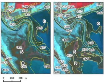
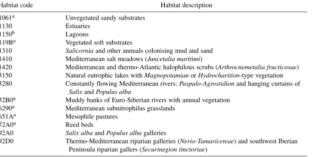
The existing habitat maps of five Greek Ramsar wetlands (artificial lake Kerkini, Amvrakikos gulf, Kotychi lagoons, lakes Koronia-Volvi, and the delta of Axios-Loudias-Aliakmonas rivers), which had been developed for the Ministry of Environment and the European Union in 2001 were updated using these methodologies. The developed methodology was proven successful in its application to these resulting habitat maps met the European and Greek national requirements (Fig. 16, Table 1).

Results revealed that GlobWetland products were a valuable contribution, but source data (enhanced satellite images) were necessary to discriminate spectrally similar habitats. Finally, the developed methodology can be modified for original habitat mapping [30].

Fig. 16The habitat map of 2001 using the original methodology and the updated habitat map using the proposed remote sensing methodology (Axios delta). Habitat codes listed in Table 1 (adapted from ref. [30]).

(22)

Table 1Habitat codes.

Habitat code Habitat description

1061^a Unvegetated sandy substrates

1130 Estuaries

1150^b Lagoons

119B^a Vegetated soft substrates

1310 Salicorniaand other annuals colonising mud and sand 1410 Mediterranean salt meadows (Juncetalia maritimi)

1420 Mediterranean and thermo-Atlantic halophilous scrubs (Arthrocnemetalia fructicosae) 3150 Natural eutrophic lakes with Magnopotamianor Hydrocharition-type vegetation 3280 Constantly flowing Mediterranean rivers: Paspalo-Agrostidionand hanging curtains of

Salixand Populus alba

32B0^a Muddy banks of Euro-Siberian rivers with annual vegetation 6290^a Mediterranean subnitrophilus grasslands

651A^a Mesophile pastures

72A0^a Reed beds

92A0 Salix albaand Populus albagalleries

92D0 Thermo-Mediterranean riparian galleries (Nerio-Tamariceteae) and southwest Iberian Peninsula riparian gallers (Securinegion tinctoriae)

aHabitats not included in Annex I of the habitats directive.

bPriority habitat type according to Annex I.

In another instance, a combination of remote sensing, field surveys, and sedimentological analysis of beach sands was used to assess changes of the shorelines of the Nile delta in general and specifically at Damietta owing to the construction of a harbour. Very dynamic coastlines, such as sections of the Nile delta coast, pose considerable hazards for human structural use and development, and rapid, replicable techniques are required to update coastline maps of these areas and monitor rates of move- ment. The synoptic capability of Landsat-TM imagery enables monitoring of large sections of coastline at relatively coarse 30 m spatial resolution. By comparing positions of the Nile delta coast in 1984, 1987, and 1990–1991, mapped using a region-growing image segmentation technique, areas of rapid change can be identified and targeted for more detailed monitoring in the field, or using higher-resolution images. Rates of erosion and deposition can be estimated crudely, and areas where change appears to be accelerating can also be identified. Areas of severe erosion along the Nile delta coast are found to be confined to the promontories of the present-day mouths of the Nile River at Rosetta and Damietta.

The results indicated that harbour construction, and, in particular, the construction of two jetties that extend out from the harbour entrance, have created a discontinuity in the eastward-moving littoral drift.

Significant shoreline advance extends a considerable distance west of the western jetty (Fig. 17a), and significant shoreline recession extends a considerable distance east of the eastern jetty (Fig. 17b).

Conventional bathymetric surveys highlight changes in the near-shore environment associated with the growth of the up-drift accretionary wedge and siltation of the harbour access channel. The synergistic use of remote sensing, bathymetric surveying, and sedimentology provides evidence that changes have affected a much larger area than predicted at the time of harbour construction [31,32].

Remote sensing has also been deemed as promising in identifying fracture zones on the Earth’s surface especially when field surveys fail to trace and identify them in arid regions, characterized by flat topography and where sand dunes extensively cover the terrain. It is deemed possible to identify the regional fractures as lineaments on remotely sensed images or shaded digital terrain models. In such research, a segment tracing algorithm (STA), for lineament detection from Landsat-7 Enhanced Thematic Mapper Plus (ETM+) imagery, and the data from the Shuttle Radar Topographic Mission (SRTM) 30 m DEM, were applied in the Siwa region (northwest of the Western Desert of Egypt). The objectives were to analyze the spatial variation in orientation of the detected linear features and its rela-

(23)

tion to the hydrogeologic setting in the area and the underlying geology, and to evaluate the perform- ance of the algorithm applied to the ETM+ and the DEM data. Detailed structural analysis and better understanding of the tectonic evolution of the area could provide useful tools for hydrologists for reliable groundwater management and development planning [33].

Remote sensing has also been used to reveal buried river channels in a number of regions worldwide, in many cases providing evidence of dramatic paleoenvironmental changes over Cenozoic time scales. Using orbital radar satellite imagery, a major paleodrainage system in eastern Libya was mapped. This paleodrainage system could have linked the Kufrah basin to the Mediterranean coast, possibly as far back as the middle Miocene. SAR images from the PALSAR sensor revealed a 900-km-long river system, which started with three main tributaries that connected in the Kufrah oasis region. The river system then flowed north and formed a large alluvial fan. The sand dunes of the Calanscio Sand Sea prevented deep orbital radar penetration and precluded detailed reconstruction of any possible connection to the Mediterranean Sea, but a 300-km-long link to the Gulf of Sirt through the Wadi Sahabi paleochannel is likely. If this connection is confirmed, and its Miocene antiquity is established, then the Kufrah River, comparable in length to the Egyptian Nile, will have important implications for the understanding of the past environments and climates of northern Africa from the middle Miocene to the Holocene [34].

Remote sensing techniques have also been combined with field investigations in order to locate and accurately characterize volcanic structures. The detection of caldera structures, apart from its usefulness in volcanological studies, is also of great interest for applied ore deposit research for epithermal precious metal mineralization in geothermal fields. Such an application was reported for the volcanic field of Lesvos Island, in which volcanic structures were difficult to recognize owing to erosion and faulting. Landsat-TM and Satellite Pour Observer la Terre Panchromatic (SPOT-Pan) satellite images as well as the DEM of the study areas were digitally processed in order to reveal specific geological characteristics related to caldera structures such as topographic caldera rims and floors, ring faults, areas of hydrothermal alteration, drainage networks, and lava domes, both internal and external to caldera structures. Six caldera structures were recognized, of which four have been identified for the first time. A combination of remote sensing and fieldwork data was used for the detection and mapping of the Miocene calderas. The relevant output images were generated from the analysis and processing of: (1) a Landsat-TM satellite image of Lesvos Island, with a spatial resolution of 30 × 30 m pixel size, acquired on 20 August 1999; (2) a SPOT-Pan satellite image of the same area, with a spatial resolution of 10 ×10 m pixel size, acquired on 12 July 1999; and (3) the DEM with a cell size of 30 m, which was obtained by digitizing the elevation contour lines of the 1:50 000 scaled topographic maps of the study Fig. 17Maps showing the changes in shoreline position to the (a) west and (b) east of Damietta Harbour, produced by automatic segmentation of Landsat-TM imagery. Shoreline positions are mapped at 1984, 1998, and 1991 (adapted from ref. [32]).

(24)

area. It is a continuous raster layer of the island, in which data values represent elevation, generated from the 30 m contours of the topographic maps. The satellite data were pre-processed in order to remove the geometric distortions and to bring the remote sensing images into registration with one another. With the use of topographic maps of the study area, the images were geometrically corrected and geo-referenced based on the Hellenic Geodetic Reference System (HGRS ’87) [35].

9. REMOTE SENSING MONITORING OF BIOTA

The tools of remote sensing have also been used, but to a lesser extent, for biological oceanography applications. One of the research fields is the mapping of sea grasses, such as the protected species Posidonia Oceanica, which is the dominant sea grass in the Mediterranean Sea and is known to affect bio-geochemical and physical processes in coastal areas. The widespread loss of this species is attributed to excessive anthropic pressure and other large-scale environmental changes. Sea grass conservation requires mapping to estimate the extent of existing stocks and to measure changes over time.

Optical remote sensing provides a cost-effective method to monitor vast areas of shallow waters that are potential P. oceanicahabitats. As part of an interdisciplinary research effort, where the effects of these sea grasses on the hydrodynamics were investigated, new technologies of reliable, fast, and effective monitoring of P. oceanicawere essential. A published method used IKONOS multispectral imagery for bottom classification in a shallow coastal area of Mallorca (Balearic Islands). After applying a super- vised classification, pixels were automatically classified in four classes: sand, rock, P. oceanica bot- toms, and unclassifiable pixels (Fig. 18). Results indicated that, in these clear waters, the spectral response of P. oceanicacan be determined to a depth of about 15 m. In order to validate the method, the image classification was compared with a bottom classification derived from an acoustical survey.

Agreement with the reference acoustic seabed classification was up to 84 % for the sampled area. Thus, spectral IKONOS image analysis was presented as an effective approach for monitoring P. oceanica meadows in most clear, shallow waters of the western Mediterranean [36].

In another study, multispectral imagery with a spatial resolution of 10 m and fused imagery with a spatial resolution of 2.5 m from the SPOT 5 satellite were used for mapping beds of P. oceanicain the Mediterranean Sea (Laganas Bay, Zakynthos, Greece, Caretta carretahabitat), where it is a dominant species. Posidonia forms monospecific beds in a structurally simple environment, where four classes can be identified: sand, photophilous algae on rock, patchy sea grass beds, and continuous sea Fig. 18Bottom types derived from the IKONOS satellite images (left) and acoustical survey (right) [36].

(25)

grass beds (Fig. 19). A direct comparison of overall accuracy between SPOT 2.5 m and SPOT 10 m revealed that this tool provided accurate mapping in both cases (between 73 and 96 % accuracy).

Although SPOT 2.5 m provided lower overall accuracy than SPOT 10 m, it is a very useful tool for the mapping of P. oceanica, as it allows the patchiness of the formations to be better taken into account [37].

A Greek research team has shown that the introduction of warm and tropical alien species in the Aegean and Ionian seas has been exacerbated by the observed warming of the eastern Mediterranean Sea. The phenomenon has accelerated after an abrupt shift in both regional and global temperatures that we detect around 1998, leading to a 150 % increase in the annual mean rate of species entry after this date. Abrupt rising temperature since the end of the 1990s has modified the potential thermal habitat available for warm-water species, facilitating their settlement at an unexpectedly rapid rate. For the statistical correlations, the following types of data were used: (A) long-term data of 149 warm alien species from 1924–2007 obtained from the list available at the Ellenic Network on Aquatic Invasive Species (ELNAIS) web site, which is archived in the Hellenic Centre for Marine Research and updated with every new record and regularly reported; (B) SST data (AVHRR, NOAA, 1985–2007); (C) northern hemisphere temperature (NHT) anomalies, obtained from the Climatic Research Unit and Hadley Centre from 1850 to 2007; and (D) regional air temperature data that were collected and provided from the meteorological stations of the Hellenic National Meteorological Service (HNMS) at 15 stations (north, middle, and south Aegean and eastern Ionian seas). The speed of alien species spreading and response to global warming is apparently much faster than temperature increase itself, presenting an important warning for the future of Mediterranean Sea biodiversity [38].

Some studies have tried to explain distributions and habitat preferences of cetaceans. In one such study, habitat use and preferences of fin whales and striped dolphins were modeled in order to provide information on critical habitats for cetaceans and meet the needs of the Pelagos Sanctuary for the Conservation of Mediterranean Marine Mammals (between southeastern France, Monaco, northwestern Italy, and northern Sardinia, and encompassing Corsica and the Tuscan Archipelago). In order to produce the desired information sighting, data collected between 1993 and 1999, explanatory physio- graphic variables (mean, range, and standard deviation of depth and slope, and distance from the near- est coastline), and remotely sensed data (SST and chl-a concentration from AVHRR and SeaWiFS sensors) were considered in the models. Generalized additive models (GAMs) were used to model the distribution of fin whales and striped dolphins in relation to these variables, and “classification and regression trees” were used for habitat characterization and predictive models. SST values were indi- cators of striped dolphin and fin whale presence, with both species showing a tendency to prefer colder Fig. 19Maps of the benthic assemblages and bottom types (Laganas Bay, pixel size 2.5 m, left, and 10 m, right) [38].