Remote Sensing of Environment

(1)

Contents lists available atScienceDirect

Remote Sensing of Environment

journal homepage:www.elsevier.com/locate/rse

Drainage basin delineation for outlet glaciers of Northeast Greenland based on Sentinel-1 ice velocities and TanDEM-X elevations

Lukas Krieger

^a,∗

, Dana Floricioiu

^a

, Niklas Neckel

^b

aRemote Sensing Technology Institute, German Aerospace Center (DLR), Oberpfaﬀenhofen, Germany

bAlfred Wegener Institute for Polar and Marine Research, Bremerhaven, Germany

A R T I C L E I N F O

Keywords:

Drainage basin Watershed Glacier catchment Monte-Carlo simulation Ice sheet

Greenland

A B S T R A C T

The drainage divides of ice sheets separate the overall glaciated area into multiple sectors. These drainage basins are essential for partitioning mass changes of the ice sheet, as they specify the area over which basin specific measurements are integrated. The delineation of drainage basins on ice sheets is challenging due to their gentle slopes accompanied by local terrain disturbances and complex patterns of ice movement. Until now, in Greenland the basins have been mostly delineated along the major ice divides, which results in large drainage sectors containing multiple outlet glaciers. However, when focusing on measuring glaciological parameters of individual outlet glaciers, more detailed drainage basin delineations are needed. Here we present for thefirst time a detailed and fully traceable approach that combines ice sheet wide velocity measurements by Sentinel-1 and the high resolution TanDEM-X global DEM to derive individual glacier drainage basins. We delineated catchments for the Northeast Greenland Ice Sheet with a modified watershed algorithm and present results for 31 drainage basins. Even though validation of drainage basins remains a difficult task, we estimated basin probabilities from Monte-Carlo experiments and applied the method to a variety of different ice velocity and DEM datasetsfinding discrepancies of up to 16% in the extent of catchment areas. The proposed approach has the potential to produce drainage areas for the entirety of the Greenland and Antarctic ice sheets.

1. Introduction

With the advance of remote sensing sensors, the mass balance estimates of Greenland and Antarctica are getting more and more accurate (Shepherd et al., 2012;Mouginot et al., 2019). Altimetry, gravi- metry and SAR-based methods are now regularly used to monitor glaciers on a large scale for a whole ice sheet or for major drainage basins (Helm et al., 2014;Schröder et al., 2019;Sasgen et al., 2012;

Groh et al., 2014; King et al., 2018;Mouginot et al., 2019). This is important to infer ice sheet wide physical processes and predict future sea level change. In these studies, glacier basins provide information about the geometric extent of the observed glacier systems and make the mass balance estimates comparable. In the present work, for the purpose of consistency, we use the terms drainage basin and glacier catchment interchangeably but always refer to the area of ice that is completely drained by a single outlet glacier. Multiple aggregated drainage basins form a drainage sector (e.g. the Northeast Greenland Ice Stream - NEGIS) whereas, on an even larger scale, the term drainage region refers to an aggregation of several drainage sectors (e.g.

Northeast Greenland).

Until now the ice sheets’drainage sectors have been mostly separated along the major ice divides. Due to the gentle slopes for large parts of the ice sheets, they have only been processed at coarse re- solutions, sometimes with additional modelled data (Hardy et al., 2000;

Lewis and Smith, 2009). A widely used dataset for drainage sectors has been published by the NASA Goddard Space Flight Center (Zwally et al., 2012,Fig. 1). It utilises data from the ICESat Geoscience Laser Altimeter System (GLAS) and is available for both Greenland and Antarctica.

Many ice sheet wide campaigns report mass balance estimates according to this delineation including the ESA/NASA ice sheet mass balance inter-comparison exercise (IMBIE) (Shepherd et al., 2012). The second assessment IMBIE-2 (Shepherd et al., 2018) included another published dataset of drainage sectors which was made available by Rignot and Mouginot (2012)and relies on an ERS/ICESat DEM in the interior of the ice sheets with additional velocity information near the coast. While these sources provide excellent basin information for mass balance investigations on a large scale, geodetic mass balance estimates from high resolution datasets with narrow swath widths such as from the TanDEM-X (TDM), Pléiades and WorldView satellite missions (Krieger et al., 2007;Gleyzes et al., 2012;Shean et al., 2016) would

https://doi.org/10.1016/j.rse.2019.111483

Received 26 March 2019; Received in revised form 7 August 2019; Accepted 17 October 2019

∗Corresponding author.

E-mail addresses:lukas.krieger@dlr.de(L. Krieger),dana.ﬂoricioiu@dlr.de(D. Floricioiu),niklas.neckel@awi.de(N. Neckel).

T

(2)

benefit from individual glacier basins that allow a more focused data collection. Previously, Mouginot et al. (2015) delineated basins for Nioghalvfjerdsfjorden (79North) and Zachariæ Isstrøm by combining ice velocity and DEM information andMouginot et al. (2019)applied a similar methodology to delineate the entire Greenland Ice Sheet into 260 individual drainage basins. Other authors reportfindings based on self assessed drainage basins in Greenland that were derived from watershed analysis assuming iceflow in the direction of the steepest slope (Felikson et al., 2017;Marzeion et al., 2012). However, the description of a detailed and fully traceable methodology for deriving basin inventories of individual outlet glaciers is still missing.

Recently available data products such as the TDM global DEM and ice sheet wide velocity measurements such as from Sentinel-1 can be employed to partition the glaciated area into individual catchments. In the following, we propose a method to delineate drainage basins for single outlet glaciers with a modiﬁed watershed algorithm based on ice surface velocity and DEM datasets.

2. Study site

The selected study site in Northeast Greenland is roughly equivalent to the drainage sectors 1.4, 2.1, 2.2, 3.1 and 3.2 as denoted byZwally et al. (2012)or to theNEsector in the dataset produced byMouginot et al. (2019). The area features marine-terminating outlet glaciers of diﬀerent sizes including 79North with one of Greenland's rare ice

shelves. Another peculiar feature is the Northeast Greenland Ice Stream (NEGIS), that reaches over 700 km in the interior of the Greenland Ice Sheet and is drained by the outlet glaciers Zachariæ Isstrøm, 79North, Kofoed-Hansen Bræ and Storstrømmen. The complexflow configura- tions of this region of the Greenland Ice Sheet with converging glaciers (L. Bistrup Bræ and Storstrømmen) as well as diverging iceflow (NEGIS into its individual outlet glaciers) present a challenging study site for the delineation of single glacier drainage basins. For the present work we selected 31 major, marine terminating outlet glaciers belonging to the Northeast part of the ice sheet (Fig. 1) and aimed at the generation of their individual catchments. The nomenclature and locations were adopted fromRignot and Mouginot (2012).

3. Datasets

We used two independent types of data to infer theflow direction of ice for the drainage basin delineation. Thefirst data source is elevation information in the form of a rasterised DEM, which was employed with the assumption that iceflows in the direction of the steepest downhill slope. Ice velocity measurements were utilised as a second type of data to account for locations where the iceflow diverts from the direction given by the steepest slope. This can happen where the downhillflow is obstructed by large bedrock features or through interaction with other ice masses at glacier junctions (Van der Veen, 2013, Chapter 4.6).

Overall, three independent DEMs and three diﬀerent ice velocity maps were used to test the consistency of the drainage basin delineations.

3.1. Surface elevation datasets

The DEM used to delineate drainage basins is the TDM global DEM, which is assembled from time series of bistatic X-band InSAR acquisitions collected by the two twin satellites TerraSAR-X and TanDEM-X (Krieger et al., 2007). Over the Greenland Ice Sheet the data was acquired between 2011 and 2014 (Wessel et al., 2016). Subsequently, a single DEM was generated by averaging all available elevation measurements weighted with their estimated height errors (Zink et al., 2014). The TDM global DEM has a nominal pixel spacing of 0.4'' (approx. 12 m) with an absolute vertical accuracy of 6.37 m given as90%

linear error over ice covered terrain (Rizzoli et al., 2017a). The DEM was chosen for the basin delineation application because of its high spatial resolution.

Two additional DEMs were used to test the consistency of the basin delineation. Theﬁrst DEM used for the intercomparison is processed from Cryosat-2 (CS-2) data acquired in the period 2012–2013 and is posted on a regular grid of 1 km × 1 km pixel spacing (Helm et al., 2014). While the elevation bias due to penetration of TanDEM-X can be > 8 m in the interior of the ice sheet (Rizzoli et al., 2017b), only a slight bias of0.2±0.2m is found overﬂat areas for CS-2 if an appro- priate retracker is used (Schröder et al., 2017). The overall accuracy of the CS-2 DEM of Greenland is slope dependent but is given as5±65m (Helm et al., 2014). The second DEM used for the intercomparison has been developed within the Greenland Ice Mapping Project (GIMP) (Howat et al., 2014). It was generated by merging elevation measurements including photogrammetry, laser- and radar altimetry. The DEM was calibrated to mean ICESat GLAS elevations acquired between 2003 and 2009 and has a posting of 90 m.

In the present work we did not investigate elevation changes that have occurred during the acquisition times of the DEMs and their possible impact on the drainage basin delineation. Instead the DEMs are assumed to represent accurate elevations of the ice sheet for their respective acquisition period. All DEMs were smoothed with a sliding averagefilter to remove longitudinal stresses and reduce the impact of local surface slope variations. The width of the filter kernel is de- termined according to multiples of the ice thickness at each point (Morlighem et al., 2017a). Kernel diameters of 20, 10 and 0 times the ice thickness have been picked to produce 3 different versions of each Fig. 1.The study site with 31 outlet glacier seed regions (magenta) of the ba-

sins listed inTable 1. Additional termini of small outlet glaciers or land terminating glaciers are marked asundeﬁned seeds (green). Drainage to other major regions of Greenland is simulated by a rough outline around the Northeast Greenland sector (red). In the background the ice surface velocity map based on S1 (GrIS-cci) superimposed on the TDM global DEM backscattering mosaic. Black lines delineate the basins afterZwally et al. (2012).

(3)

DEM. For the remainder of the paper the versions are suﬃxed with20H, 10Hand0H. All results reported in our paper use20Has suggested in Paterson (2016, Chapter 8.7.2) while an additional example of the smoothing kernel eﬀect on the basin delineation is given in the Sup- plement (Fig. S1).

3.2. Ice velocity datasets

To supplement surface elevation data, we used surface velocity derived through oﬀset tracking of Sentinel-1 (S-1) SAR amplitude backscattering images. A multi-annual Sentinel-1 ice velocity map of Greenland was produced within the Greenland Ice Sheet project of ESA's Climate Change Initiative (GrIS-cci) Programme (Nagler et al., 2015). We obtained the geocoded velocity product for the time period Oct. 2014–Apr. 2019 and used velocity components with a posting of 250 m that we termGrIS-ccivelocities.

We employed two additional surface velocity datasets to compare the resulting drainage basins. Thefirst of these velocity maps was also derived by Sentinel-1 offset tracking and incorporates 2607 image pairs acquired over Northeast Greenland during the winters of 2016, 2017 and 2018. The processing includes mosaicking of S-1 TOPS burst SLC data, co-registration between 6-day repeat passes based on precise orbit information, offset estimation in range and azimuth direction, a pro- jection into a polar stereographic coordinate system assuming surface parallel ice flow and a three step filtering procedure (Lüttig et al., 2017). Thefinal mosaic is posted at 250 m and small data gaps arefilled via an inverse distance interpolation scheme. In the following this velocityfield is denoted asAWI-S1velocities. Note thatAWI-S1velocities andGrIS-cciare partially based on the same S-1 acquisitions but were processed separately. The second additional ice velocity dataset used in the intercomparison is distributed within the MEaSUREs project (Joughin et al., 2016). This velocity map has been generated by combining speckle- and feature tracking techniques applied at the ice sheet margins together with InSAR measurements for the ice sheet interior.

The used acquisitions fall within the time of 1995 and 2015 and stem from multiple SAR sensors (ERS-1/2, RADARSAT, ALOS, TerraSAR-X) as well as Landsat 8. The MEaSUREs product is also posted at 250 m (Joughin et al., 2017).

3.3. Ice classiﬁcation mask

In order to restrict the processing to the ice sheet area we used the Land Ice and Ocean Classification Mask product of the MEaSUREs GIMP project (Howat et al., 2014). This data set provides a complete land ice, ice free terrain and ocean classification mask for the Greenland Ice Sheet that was mapped using a combination of Landsat 7 ETM+ pan- chromatic band imagery and RADARSAT- 1 SAR amplitude images acquired between 1999 and 2002. We modified the IceMask layer of the product which includes the ice shelves by eliminating the small ice caps and glaciers at the Greenland periphery that are not connected to the ice sheet and applied the watershed processing to the remaining ice coverage.

3.4. Selection of seed regions

Seed locations are required for each catchment in order to start the partitioning of the ice sheet into drainage basins. The seed regions are defined on the ice of the termini marking areas upstream from the glacier front. Thus the seed regions belong to the part of the tongue where ice is discharged into the ocean or where the glacier is terminating on land. The largest seed regions for the study site are visualized inFig. 1. We have defined three types of seed regions needed to support our processing: (1) on each terminus of the 31 marine terminating glaciers considered for catchment delineation (2) several seed regions of small unnamed glaciers thatflow also to the ice sheet margin and (3) a large one located along the ice divides outside the rough outline of the

complete Northeast Greenland drainage region. Regions of type (1) and (2) act as sinks in the ice sheet'sﬂow system, while region (3) simulates the glaciers draining into the adjacent West and Southeast Greenland regions.

4. Methods

For the delineation of individual glacier catchment areas, a classical flood-filling watershed algorithm (Beucher et al., 1992) was adapted to use both elevation and ice velocity data. In this way, we aim at a more reliable separation of glaciers in fast moving areas than by utilising only a DEM. All datasets were resampled to the same grid of 250 m pixel spacing by a cubic spline interpolation before the start of the processing, which inherently specifies the pixel spacing at which the independent parts of the algorithm operate.

4.1. Watershed algorithm

The watershed algorithm is an image processing transformation whose name refers to the geological watershed and which is widely used for various image segmentation purposes (Sonka et al., 2014, Chapter 6.3.4). When operating on a DEM and associated seed points, the watershed algorithmﬁnds the lines separating adjacent drainage basins (Beucher et al., 1992; Vincent and Soille, 1991). We used an implementation of the watershed algorithm which utilises a priority queue that is sorted by minimum elevation (Barnes et al., 2014). During the algorithm run, pixels adjacent to each seed point are entered into the queue and are processed in the order of increasing elevation. This ensures a pixel-wise processing, with regions evolving from given seed points to form a partitioning of the area of interest. Finally, the drainage divides of the DEM are represented by the boundaries of the basins generated by the watershed algorithm.

One approach to delineate basins is to apply the watershed algorithm only on the ice sheet DEM and the seeds corresponding to its outlet glaciers. However,Rignot et al. (2000)point out that in order to correctly delineate catchments in fast moving areas, ice surface velocities must be taken into account in addition to the slope information provided by the DEM. As directional errors in the velocity measurements are more related to the velocity magnitude than to absolute elevation, we adopted a method similar toMouginot et al. (2015)which uses thresholds for the ice velocity magnitude to separate between ice ﬂow and surface slope direction instead.

4.2. Streamline calculation

In order to accommodate velocity information in the traditional watershed algorithm, we calculated streamlines from the north and east velocity components. They describe the trajectory that imaginary par- ticles would take in the given velocity field. We produced discrete streamlines with the procedure described byCabral and Leedom (1993) but restricted the calculation to areas moving faster than a given absolute velocity threshold, while slower areas were discarded. The streamline computation is included in the modified watershed algorithm starting from a given pixel and ending once the streamline ex- tends beyond the coverage of the velocityfield or if the streamline merges with an already existing one. An example for the NEGIS sector is depicted inFig. 2.

4.3. Catchment delineation

To combine the directional information from iceflow with the slope information, the traditional watershed algorithm was modified to dis- regard slope information in areas of fast moving ice where the velocity magnitude exceeds a pre-defined threshold. Instead, every time such an area is encountered, the entire labelledflow line (as derived in section 4.2) is included in the currently processed drainage area and its entire

(4)

neighbourhood is entered in the priority queue of the watershed algorithm.

The choice of seed regions controls the partitioning of the ice-covered area into drainage basins. A catchment was generated for every seed region of type (1) (Section 3.4) with a unique seed label. This partitions the entire glaciated area into a number of basins equal to the number of different seed region labels. All additional smaller glaciers of type (2) and the adjacent major drainage region (3) were assigned the undefinedlabel. If an additional drainage basin is desired in a part of the ice sheet that drains through anundefinedseed region of type (2), an additional labelled outlet glacier seed (1) can be placed and the modified watershed algorithm can be re-run.

In order to mitigate the propagation of local errors in the datasets to global errors in the drainage delineation we applied a Monte-Carlo method adding Gaussian noise with zero mean to both the DEM and the ice velocity components as well as the used ice velocity threshold. In this settingN=10000runs of the algorithm were performed using the pixel-wise uncertainties for thexandyice velocity components. The standard deviation for the DEM and ice velocity threshold were set to

=

σDEM 10mandσ_t=2ma⁻¹, respectively. Subsequently, each pixel was assigned the basin label of maximal occurrence in all runs and a probability measurement was calculated based on the percentage of total Monte-Carlo runs for which that pixel was included in that

particular basin. Noisy delineations at the basin boundaries were cleaned by restricting the number of connected clusters per label to 1.

5. Selection of the ice velocity magnitude threshold

For slow moving ice, the reduced SNR in the amplitude correlation functions of the speckle tracking measurements can lead to a degradation of theﬂow direction estimate. Additionally, there are arte- facts in the velocity measurement stemming from an active ionosphere.

Even though the velocity vector can be measured more precisely with InSAR and higher quality velocity maps with smallerflow direction uncertainties can be produced, small scale ionospheric perturbations still remain in the velocity measurements after the ionospheric cor- rection by the split-spectrum method (Gomba et al., 2016,2017). At the ice divides, the errors of the velocity components are in the order of 5 m a⁻¹. In these areas, the direction of the steepest surface slope can be derived more accurately as long as the assumption of downhillflow along smoothed DEMs is valid. On the other end of the velocity range, fast moving ice does not alwaysflow in the direction of the steepest slope if there exists an instability orflow change. Here, the actualflow direction can be precisely derived from the offset tracking results. By using flow directions instead of slope information and vice versa in regions of high and low ice velocities, the drawbacks of both types of data can be overcome.

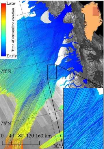
The criterion whether the slope-based or velocity-basedflow directions should be utilised was predicated on the comparison between two angles. Both types offlow directions were expressed as vectors with unit length and the angular argument was used. The iceflow angle given byGrIS-ccivelocities and the aspect angle (direction of steepest slope) of the TDM global DEM were computed over the entire Northeast Greenland region. The mean difference between these angles as well as their correlation are calculated over velocity magnitude bins that contain an equal number of points (Fig. 3a). The velocity of 13.67 m a⁻¹at maximum correlation was chosen as the threshold for the modified Fig. 2.The streamlines for the NEGIS drainage sector colour coded by the time

of creation during the modiﬁed watershed algorithm. The streamlines have been calculated on the complete averaged GrIS-cci velocity dataset for ice speeds exceeding 13.67 m a⁻¹. Dark-blue refers to streamlines originating from low altitudes close to the coast propagating to the upper part of NEGIS. Light- blue to red colours are associated to streamlines starting at higher elevations.

The inset shows streamlines clearly separating NEGIS into two arms. In the background the TDM SAR backscattering amplitude mosaic.

Fig. 3.(a) Correlation and mean difference of the TanDEM-X global DEM aspect angle (direction of steepest slope) and theflow angle ofGrIS-ccivelocity vectors. The comparison is carried out over the entire Northeast Greenland ice sheet area for velocity bins that contain an equal number of points. At a velocity of 13.67 m a⁻¹the maximum correlation is reached (red dot). (b) The uncertainty of theflow direction for the 3 different velocity maps.

(5)

watershed algorithm indicating the use of DEM or ice velocities. Above 13.67 m a⁻¹we expect the direction from velocity information to be accurate to the true iceﬂow direction and below the threshold the slope information is trusted.Fig. 3b shows this degradation of theﬂow direction measurement with decreasing ice velocity magnitude.

For the TDM global DEM and GrIS-cci velocity combination the angle correlation reaches a maximum of 0.98 while the mean difference of the two angles is 0.5^∘at this peak. Angle differences up to 6^∘occur in regions of fast and slow ice movement. For fast flowing ice (> 300 m a⁻¹) correlation of approx. 0.85 is found while slower ice (< 2 m a⁻¹) has correlation values of less than 0.6 indicating a mis- alignment between the iceflow and surface slope directions. It should be noted that the correlation stays close to 1 in a broad range of velocities, indicating that the exact threshold can be variable and plays a limited role in the basin delineation.

The angle analysis was performed for the diﬀerent DEM and velocity dataset combinations, yielding similar results with correlation patterns peaking between 13 m a⁻¹ and 44 m a⁻¹ (Supplement, Fig.

S2). For the InSAR-based velocity map, correlations close to 1 are maintained for slower ice velocities even though the highest angle correlations are still found between 10 m a⁻¹and 44 m a⁻¹. We applied the respective velocity thresholds for the diﬀerent input dataset combinations and modiﬁed the threshold by adding Gaussian noise for each individual Monte-Carlo run. This limits the dependence of the exact threshold on the delineation.

6. Results

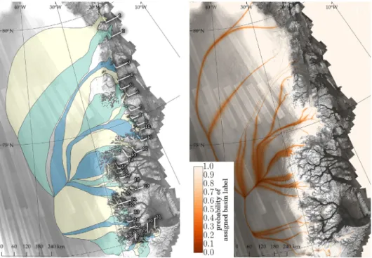
We used the combination TDM global DEM20HandGr-IS-ccivelocities with 250 m pixel spacing as input dataset for the modiﬁed watershed algorithm and seed regions for its initialization. The resulting delineations of the 31 drainage basins are shown inFig. 4a. The streamline calculation performed during the algorithm runs over areas where the ice velocity exceeds the previously estimated threshold (TDM-GrIS-cci: 13.67 m a⁻¹). The probability estimates for each assigned basin label resulting from the Monte-Carlo simulation with

=

N 10000runs are shown inFig. 4b. The characteristics of the generated basins are summarised in Table 1 in decreasing order of their

drainage area.

7. Intercomparison with other DEM and velocity products Additional to the results presented above, basin delineations with all other input data combinations of the DEMs (TDM, GIMP, CS-2) and ice velocities (GrIS-cci, MEaSUREs, AWI-S1) were generated for intercomparison purposes. This way we gain insight if the errors that are inherent to each dataset have an eﬀect on our proposed delineation.

In order to quantify the similarity between the results based on diﬀerent datasets, we calculate the Jaccard indexJfor each combination of two drainage basin delineation results A={A A1, 2, ,…An} and

= …

B { ,B B₁ ₂, ,B_n}(Jaccard, 1912). Over the whole region of interest we divide the number of commonly labelled pixels in both delineations by the overall number of labelled pixels.Ak,Bk are therefore holding all pixels labelled for glacierkand… denotes the number of pixels in the given set. The Jaccard index is 1 ifAandBdelineations are in perfect agreement and decreases with their spatial dissimilarity.

=

∪ ∩

∪ J =

A B A B

k n

k k

1

(1) The Jaccard indices of the various input data combinations range from 0.81 to 0.98 (Table 2). Discrepancies in the delineation of the basin boundaries are visible in Fig. 5and are due to diﬀerent time spans, error sources and limitations of each of the input data products.

All delineations using the GIMP DEM perform closer to that of the TDM global DEM compared to those using the CS-2 DEM. The lower Jaccard index of 0.90 when comparing catchment delineations based on the TDM global DEM to the ones based on CS-2 (both usingGrIS-ccivelocities) is caused by the low resolution and poor performance of CS-2 in areas of complex topography at the margin of the Greenland Ice Sheet (Fig. 5 b,c). As the flood-filling watershed algorithm processes the margins early in the labelling process, errors can propagate towards the interior of the ice sheet and thefinal difference in basin area can be substantial. The results using the GIMP DEM are in better agreement (Jaccard index 0.98) with the TDM global DEM based basins (both usingGrIS-ccivelocities) since the resolution of both products is high

Fig. 4.(a) Northeast Greenland Ice Sheet region divided into drainage basins of the 31 outlet glaciers inTable 1. (b) The pixel-wise probability of the assigned basin label for each basin. In the background the SAR backscattering amplitude layer of the TDM global DEM.

(6)

enough to capture topographic details in steep areas. An area of 9% of all basins in the sector is labelled diﬀerently when substitutingGrIS-cci with the MEaSUREs velocity dataset, whereas the AWI-S1velocities show dissimilarities of 11% to theTDM-GrIS-cciresult. In general it can also be observed that greatest discrepancies between the datasets in Fig. 5a are located in the basins that are delineated with low probabilities inFig. 4b.

Smoothing the DEM before watershed processing has less impact than the selection of diﬀerent input datasets. The lowest Jaccard index for delineations with10Haverage kernels is 0.94 while no smoothing shows a minimum Jaccard index of 0.90 (Table 3). A decreasing trend of basin similarities with smaller smoothing kernels can be observed for each combination of input datasets. Without smoothing the TDM global DEM, the resulting discrepancies are 6% of the area compared to the presented delineation using a smoothing kernel of20H.

8. Discussion

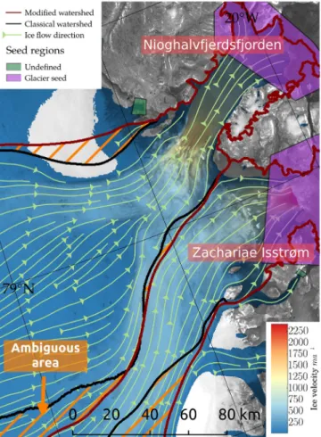
The importance of using additional velocity information for watershed delineation is illustrated at the boundary between 79North and Zachariæ Isstrøm (Fig. 6). We compare the classical drainage divide based solely on the TDM global DEM with the border obtained when additional iceflow directions are used. In agreement at low altitudes the watershed lines resulting from the two methods start to deviate from each other with increasing elevation. In this area the ice speed is > 300 m a⁻¹and the assumption that velocity vectors point down- slope does not hold. This can be a result of an interaction of the two branches of NEGIS, the disturbance of iceflow by a large subglacial bedrock feature or an ice sheet imbalance. The iterative nature of the watershed algorithm causes preceding errors during processing to propagate to areas of higher elevations and thus the resulting watershed lines can deviate significantly from each other. As revealed by theflow lines inFig. 6, an approx. 20 km wide part of NEGIS is incorrectly attributed to Zachariæ Isstrøm and the ice area which feeds that part of Table 1

Drainage basin areasA for each numbered glacier as inFig. 1based on theTDM-GrIS-cciinput dataset combination. The ice volumeVis calculated with the Bedmachine dataset (Morlighem et al., 2017a,b). Area fractionsA_fracare given with respect to the total Greenland Ice Sheet area (Howat et al., 2014). Minimum and maximum areaAminandAmaxfor a basin are given based on the extrema in the delineations resulting from all other input dataset combinations. Area diﬀerencesΔA are reported for corresponding catchments inMouginot et al. (2019)and sea level equivalents (SLE) were calculated.

# Glacier name A[km ]² A^frac[ %] Amin[km ]2 Amax[km ]2 V[km ]³ ΔA[km ]² SLE [m]

1 Nioghalvfjerdsfjorden (79North) 107791 6.28 107774 111884 227424 −2559 0.58

2 Zachariæ Isstrøm 84398 4.92 83879 96547 200199 −6864 0.51

3 Kofoed-Hansen Bræ 74686 4.35 45057 90473 173136 – 0.44

22 Daugaard-Jensen 48369 2.82 47847 51225 110810 −1557 0.28

4 Storstrømmen 28859 1.68 23353 37444 53872 – 0.14

12 Waltershausen Gletscher 23141 1.35 17354 25490 34821 −990 0.09

5 L. Bistrup Bræ 21868 1.27 21652 29701 24648 233 0.06

14 Gerard de Geer Gletscher 15735 0.92 11965 19903 19932 2267 0.05

11 Wordie Gletscher 14995 0.87 10240 17774 21686 4771 0.05

26 Vestfjord Gletscher 11806 0.69 11285 13082 11506 590 0.03

25 Rolige Gletscher 9917 0.58 9146 12172 18003 – 0.05

20 F. Graae Gletscher 7288 0.42 37 7525 12754 1781 0.03

16 Nordenskiöld Gletscher 5209 0.30 1006 5545 6967 1132 0.02

24 Unnamed Hare Fjord 5170 0.30 1375 6189 9683 – 0.02

13 Adolf Hoel Gletscher 4323 0.25 2577 7798 1845 −4773 0.00

15 Jættegletscher 3819 0.22 1158 5407 3154 −1710 0.01

29 Magga Dan Gletscher 3768 0.22 3582 4015 2120 −672 0.01

23 Eielson Gletscher 3700 0.22 2555 5083 1404 – 0.00

19 Violingletscher 3432 0.20 760 3432 1162 – 0.00

6 Soranerbræen Gletscher 2956 0.17 2545 5586 2655 – 0.01

7 Einar Mikkelsen Gletscher 2263 0.13 23 2263 1597 – 0.00

17 Hisinger Gletscher 1939 0.11 1939 15897 1568 −932 0.00

18 Wahlenberg Gletscher 1559 0.09 1079 1699 988 – 0.00

31 Bredegletscher 1546 0.09 1485 1690 254 276 0.00

28 Kista Dan Gletscher 1524 0.09 822 1585 934 – 0.00

8 Heinkel Gletscher 1093 0.06 253 1100 417 – 0.00

30 Sydbræ 1072 0.06 997 1091 148 −93 0.00

27 Unnamed Vestfjord S 931 0.05 798 1308 250 – 0.00

9 Tvegegletscher 924 0.05 771 960 130 – 0.00

10 Pasterze 743 0.04 715 761 16 – 0.00

21 Charcot Gletscher 580 0.03 560 728 360 −572 0.00

Table 2

Jaccard indices for all combinations of input DEMs and ice velocity datasets compared to the basins based on the TanDEM-X global DEM and theGrIS-ccivelocities.

The comparison is always performed with respect to delineation results applying the same DEM smoothing kernel with sizes equal to multiples of the ice thickness (20H, 10H, 0H).

Drainage basin delineation identiﬁer Input DEM & IV dataset combinations

TDM GIMP CS-2

GrIS-cci MEaSUREs AWI-S1 GrIS-cci MEaSUREs AWI-S1 GrIS-cci MEaSUREs AWI-S1

TDM-GrIS-cci-20H 1.00 0.91 0.89 0.98 0.89 0.89 0.90 0.87 0.84

TDM-GrIS-cci-10H 1.00 0.91 0.89 0.98 0.85 0.87 0.90 0.87 0.83

TDM-GrIS-cci-0H 1.00 0.93 0.88 0.96 0.84 0.85 0.88 0.87 0.81

(7)

the ice stream is misclassified. One has to note that including iceflow direction allows to delineate drainage basins for the current state of the ice sheet and in this setting the classical watershed processing fails to properly delineate the catchments. However, using current ice velocities does not allow to delineate retroactively the drainage basins for a past ice sheet in balanced state, since the velocity patterns change in response to ice sheet imbalances. Nonetheless, using only a smoothed DEM assumes an ice sheet in balance which is not the case for the recent DEMs and the basins boundaries may differ substantially (Supplement, Fig. S3). If instead of ice flow catchments the research objective are basins for surface water routing, one must use an unfiltered, high resolution DEM only, ignore ice velocity and include land areas in the processing.

The choice of seed regions is an important step for the creation of drainage basins, because it has a direct impact on their delineation. This eﬀect can be observed at the additionalundeﬁnedseeds (Fig. 1), which

eﬀectively exclude areas from the drainage delineation that are not directly drained through one of the selected outlet glaciers of type (1).

InFig. 6one such example is shown adjacent to the 79North basin.

Changing the extent of this seed region has the potential to alter the entire 79North basin area by thousands of km². The same problem exists for all adjoining seed regions located directly at the ice margin where the ice/land interface has to be manually distributed to the neighbouring glaciers. Because the processing was restricted to the glaciated area only and most of the seed regions are located in clearly separated fjords this is a minor problem for large parts of the ice sheet.

Here, the shape of the seed polygons has no eﬀect on the delineation.

Setting the seed regions requires a decision on which outlet glaciers should be assigned to a common drainage system. If in doubt we advise to create separate seed regions for the glaciers in question with the possibility to merge the basins retroactively. Similarly, if glacial surges Fig. 5.The basin boundaries resulting from all input DEM and velocity dataset

combinations. Inset (a): different delineations that originate from diverging ice flow directions at lower elevations. (b) and (c): places whereCS-2delineations are at different locations than the GIMP and TDM based boundaries. In the background the TDM SAR backscattering amplitude mosaic.

Table 3

Jaccard indices for the comparison of drainage basin delineations using the DEM smoothed with the 20H kernel versus the 10H smoothed and 0H (original) DEM.

DEM smoothing kernel size Input DEM & IV dataset combinations (20H)

TDM GIMP CS-2

GrIS-cci MEaSUREs AWI-S1 GrIS-cci MEaSUREs AWI-S1 GrIS-cci MEaSUREs AWI-S1

10H 0.98 0.98 0.96 0.97 0.94 0.96 0.98 0.99 0.97

0H 0.94 0.93 0.90 0.94 0.90 0.91 0.96 0.97 0.93

Fig. 6.Watershed lines separating the two glaciers 79North and Zachariæ Isstrøm derived by the classical watershed algorithm based solely on DEM information (black line) compared to the basin boundary when additional ice velocity is used (red line). The disagreement between the drainage divides leads to an ambiguous area which according to the iceﬂow direction (green arrows)is misclassiﬁed by the classical watershed procedure. In the background the TDM SAR backscattering amplitude mosaic.

(8)

are suspected, questionable basins should also be combined after the watershed delineation using insight from the accompanying probability estimates.

Apart from the seed selection, the implementation of the flood- filling watershed algorithm is deterministic and the errors of the basin delineation are a result of errors in the input data. Inflood-filling watershed algorithms, localised errors of the input dataset can propagate to global errors in thefinal segmentation. It is therefore challenging to quantify the quality of the drainage basin delineations directly from the local, pixel-wise uncertainties of the input data (Straehle et al., 2012).

Instead, we investigate the uncertainty of the basin boundaries by performing Monte-Carlo experiments using standard deviations reported for the 3 individual velocity maps. In the case of the DEM, the uncertainties are diﬃcult to evaluate because of the ice thickness dependent smoothing.σDEMwas set conservatively and likely exceeds the expected error in the DEM datasets. The reported probability map for the basins therefore represents an upper boundary. Additionally, a small uncertainty ofσ_t=2ma⁻¹was applied to the velocity threshold derived in section5to limit its eﬀect on the delineation.

While the overall height accuracy of the TDM global DEM is given with 3.49 m it decreases to 6.37 m over ice covered regions (Rizzoli et al., 2017a). This eﬀect can be attributed to the SAR signal penetration. In the interior of the Greenland Ice Sheet the penetration bias at X- band compared to ICESat measurements can be > 8 m with a mean elevation bias of 5.4 m for the dry snow zone (Rizzoli et al., 2017b).

However, the rather gradual spatial variability of the penetration bias implies a very small effect on the relative height accuracy at regional scale and the related delineation of ice divides. Nevertheless, with the presented methodology it is also possible to use merged DEM information from different sources like the TDM global DEM at lower elevations combined with CS-2 elevations for the interior of the ice sheet to minimize possible effects of the penetration bias. When performing this scenario with substituted TDM elevations above 2000 m no major differences have been found to using only TDM elevations (Jac- card index of 0.99, Supplement,Fig. S4).

Similar results are found when the modified watershed algorithm is run with surface velocityfields produced by different groups (Table 2).

However, it should be noted that here we rely on multi year averages in order to increase the accuracy of the speckle tracking results in slowly moving areas.

Overall, the catchment area results inTable 1show differences to the values found in the literature. According to ourfindings, the glacier catchments of 79North and Zachariæ Isstrøm are 2559 km² and 6864 km²smaller compared to the corresponding basins inMouginot et al. (2019) after correcting for the different seaward basin extent.

Relative to the total basin area, larger discrepancies are found for Wordie Gletscher (32%) or Adolf Hoel Gletscher (110%). Two large basins of the surge-type Storstrømmen and Kofoed-Hansen Bræ are not included in the comparison because their catchments are combined in Mouginot et al. (2019). The discrepancies can arise for various reasons, including the choice of the DEM, the velocity dataset or the used methodology. Moreover, a clear deﬁnition is needed for the points of drainage to land and ocean, i.e. our seed regions. The mentioned sources do not describe the methodology in detail. The present study based on independent datasets can reliably delineate basins of certain glaciers like in the case of 79North where the maximal area discrepancy (Amax−Amin) of all input dataset combinations is only 4110 km² (0.4%) (Table 1). 79North shows clearly deﬁned basin boundaries with low variability. Other catchments however (e.g. Storstrømmen and Kofoed-Hansen Bræ), are derived with low probability (Fig. 4b).

9. Conclusion

Individual glacier catchments support a quantification of glacier changes for a specified region and are therefore an important tool in the field of glaciology and hydrology. Moreover, standardised basins allow

for a direct comparison of study results and lead to more robust estimates of glacier mass balances. We developed a method based on objective decision criteria for tracing basin outlines and applied it for the Northeast Greenland region. By using combined DEM and velocity information with a modified watershed algorithm, a new partitioning of the region into 31 individual glacier catchments has been performed. As an independent, high accuracy data base for full validation of the results is lacking, quality assessment was supported by performing an intercomparsion with different input data combinations of DEMs and ice velocity products showing discrepancies of up to 16% in the extent of the catchment areas. The quality of the presented results was further assessed by a probability measure from additional Monte-Carlo experiments. Compared to watershed delineations using only a DEM, there are however major differences in reported drainage areas for certain glaciers, showing that previous approaches on ice sheets de- livered different basin boundaries not fully matching the present day ice sheet conditions. We suggest that catchment delineations from DEMs have to be supported by ice velocity maps and seed regions.

Given high resolution elevation measurements like the TanDEM-X global DEM and ice sheet wide ice velocity data like those provided by Sentinel-1 as well as basin starting points, the developed method has the potential to produce fully traceable outlines of drainage basins for entire Greenland and Antarctica. As ice sheet velocities are known to experience seasonal or multiyear variations, there is a possibility that also drainage areas are affected by such changes. Therefore, repeated investigations of glacier drainage systems should be carried out in the future with multi-temporal velocity datasets and accurate, high-resolution DEMs. Moreover, the procedure is also directly applicable on smaller scales for the delineation of ice divides between outlet glaciers of ice caps and icefields. It can be used to refine and update glacier inventories like the Randolph Glacier Inventory, e.g. by adding separate basins for each glacier on continuous ice bodies (RGI Consortium, 2017).

Acknowledgements

This research was supported by the Deutsche Forschungsgemeinschaft (DFG, FL 848/1-1). N.N. has received funding from the European Union's Horizon 2020 research and innovation programme under grant agreement No 689443 via project iCUPE (Integrative and Comprehensive Understanding on Polar Environments). The TanDEM-X global DEM tiles were provided by DLR under the research proposal DEM_GLAC0671 ©DLR 2017. We thank ENVEO GmbH for providing the multi-annual ice velocity map.

Appendix A. Supplementary data

Supplementary data to this article can be found online athttps://

doi.org/10.1016/j.rse.2019.111483.

References

Barnes, R., Lehman, C., Mulla, D., 2014. Priority-ﬂood: an optimal depression-ﬁlling and watershed-labeling algorithm for digital elevation models. Comput. Geosci. 62, 117–127.

Beucher, S., et al., 1992. The watershed transformation applied to image segmentation.

Scanning Microsc. Suppl 299–299.

Cabral, B., Leedom, L.C., 1993. Imaging vectorﬁelds using line integral convolution. In:

Proceedings of the 20th Annual Conference on Computer Graphics and Interactive Techniques, pp. 263–270 ACM.

Felikson, D., Bartholomaus, T.C., Catania, G.A., Korsgaard, N.J., Kjær, K.H., Morlighem, M., Noël, B., Van Den Broeke, M., Stearns, L.A., Shroyer, E.L., et al., 2017. Inland thinning on the Greenland ice sheet controlled by outlet glacier geometry. Nat.

Geosci. 10, 366.

Gleyzes, M.A., Perret, L., Kubik, P., 2012. Pleiades system architecture and main per- formances. Int. Arch. Photogr. Remote Sens. Spat. Inf. Sci. 39, 537–542.

Gomba, G., Parizzi, A., De Zan, F., Eineder, M., Bamler, R., 2016. Toward operational compensation of ionospheric eﬀects in SAR interferograms: the split-spectrum method. IEEE Trans. Geosci. Remote Sens. 54, 1446–1461.

Gomba, G., Rodríguez González, F., De Zan, F., 2017. Ionospheric phase screen

(9)

compensation for the Sentinel-1 TOPS and ALOS-2 ScanSAR modes. IEEE Trans.

Geosci. Remote Sens. 55, 223–235.

Groh, A., Ewert, H., Rosenau, R., Fagiolini, E., Gruber, C., Floricioiu, D., Abdel Jaber, W., Linow, S., Flechtner, F., Eineder, M., et al., 2014. Mass, volume and velocity of the Antarctic Ice Sheet: present-day changes and error eﬀects. Surv. Geophys. 35, 1481–1505.

Hardy, R., Bamber, J., Orford, S., 2000. The delineation of drainage basins on the Greenland ice sheet for mass-balance analyses using a combined modelling and geographical information system approach. Hydrol. Process. 14, 1931–1941.

Helm, V., Humbert, A., Miller, H., 2014. Elevation and elevation change of Greenland and Antarctica derived from CryoSat-2. Cryosphere 8, 1539–1559.

Howat, I.M., Negrete, A., Smith, B., 2014. The Greenland Ice Mapping Project (GIMP) land classiﬁcation and surface elevation data sets. Cryosphere 8, 1509–1518.

Jaccard, P., 1912. The distribution of theﬂora in the alpine zone. New Phytol. 11, 37–50.

Joughin, I., Smith, B.E., Howat, I.M., 2017. A complete map of Greenland ice velocity derived from satellite data collected over 20 years. J. Glaciol. 1–11.

Joughin, I., Smith, B.E., Howat, I.M., Scambos, T.A., 2016. MEaSUREs Multi-Year Greenland Ice Sheet Velocity Mosaic, Version 1. Boulder, Colorado USA. NASA National Snow and Ice Data Center Distributed Active Archive Center.

King, M.D., Howat, I.M., Jeong, S., Noh, M.J., Wouters, B., Noël, B., van den Broeke, M.R., 2018. Seasonal to decadal variability in ice discharge from the Greenland Ice Sheet.

Cryosphere 12, 3813–3825.https://doi.org/10.5194/tc-12-3813-2018.

Krieger, G., Moreira, A., Fiedler, H., Hajnsek, I., Werner, M., Younis, M., Zink, M., 2007.

TanDEM-X: a satellite formation for high-resolution SAR interferometry. IEEE Trans.

Geosci. Remote Sens. 45, 3317–3341.

Lewis, S.M., Smith, L.C., 2009. Hydrologic drainage of the Greenland ice sheet. Hydrol.

Process. 23, 2004–2011.

Lüttig, C., Neckel, N., Humbert, A., 2017. A combined approach forﬁltering ice surface velocityﬁelds derived from remote sensing methods. Remote Sens. 9, 1062.

Marzeion, B., Jarosch, A., Hofer, M., 2012. Past and future sea-level change from the surface mass balance of glaciers. Cryosphere 6, 1295–1322.

Morlighem, M., Williams, C.N., Rignot, E., An, L., Arndt, J.E., Bamber, J.L., Catania, G., Chauché, N., Dowdeswell, J.A., Dorschel, B., et al., 2017a. Bedmachine v3: complete bed topography and ocean bathymetry mapping of Greenland from multibeam echo sounding combined with mass conservation. Geophys. Res. Lett. 44.

Morlighem, M., Williams, C.N., Rignot, E., An, L., Arndt, J.E., Bamber, J.L., Catania, G., Chauché, N., Dowdeswell, J.A., Dorschel, B., et al., 2017b. Ice Bridge Bed Machine Greenland, Version 3. Boulder, Colorado USA. NASA National Snow and Ice Data Center Distributed Active Archive Center.

Mouginot, J., Rignot, E., Bjørk, A.A., van den Broeke, M., Millan, R., Morlighem, M., Noël, B., Scheuchl, B., Wood, M., 2019. Forty-six years of Greenland Ice Sheet mass balance from 1972 to 2018. Proc. Natl. Acad. Sci. 116, 9239–9244.https://doi.org/10.1073/

pnas.1904242116.URL: https://www.pnas.org/content/116/19/9239.

Mouginot, J., Rignot, E., Scheuchl, B., Fenty, I., Khazendar, A., Morlighem, M., Buzzi, A., Paden, J., 2015. Fast retreat of Zachariæ Isstrøm, northeast Greenland. Science 350, 1357–1361.

Nagler, T., Rott, H., Hetzenecker, M., Wuite, J., Potin, P., 2015. The Sentinel-1 mission:

new opportunities for ice sheet observations. Remote Sens. 7, 9371–9389.

Paterson, W.S.B., 2016. The Physics of Glaciers. Elsevier.

RGI Consortium, 2017. Randolph Glacier Inventory–A Dataset of Global Glacier Outlines: Version 6.0. Technical Report, Global Land Ice Measurements from Space.

Digital Media, Colorado, USA.

Rignot, E., Buscarlet, G., Csatho, B., Gogineni, S., Krabill, W., Schmeltz, M., 2000. Mass balance of the northeast sector of the Greenland ice sheet: a remote-sensing per- spective. J. Glaciol. 46, 265–273.

Rignot, E., Mouginot, J., 2012. Iceﬂow in Greenland for the international polar year 2008–2009. Geophys. Res. Lett. 39.

Rizzoli, P., Martone, M., Gonzalez, C., Wecklich, C., Borla Tridon, D., Bräutigam, B., Bachmann, M., Schulze, D., Fritz, T., Huber, M., et al., 2017a. Generation and performance assessment of the global TanDEM-X digital elevation model. ISPRS J.

Photogr. Remote Sens. 132, 119–139.

Rizzoli, P., Martone, M., Rott, H., Moreira, A., 2017b. Characterization of snow facies on the Greenland Ice Sheet observed by TanDEM-X interferometric SAR data. Remote Sens. 9, 315.

Sasgen, I., van den Broeke, M., Bamber, J.L., Rignot, E., Sørensen, L.S., Wouters, B., Martinec, Z., Velicogna, I., Simonsen, S.B., 2012. Timing and origin of recent regional ice-mass loss in Greenland. Earth Planet. Sci. Lett. 333–334, 293–303.https://doi.

org/10.1016/j.epsl.2012.03.033.

Schröder, L., Horwath, M., Dietrich, R., Helm, V., van den Broeke, M.R., Ligtenberg, S.R.M., 2019. Four decades of Antarctic surface elevation changes from multi-mission satellite altimetry. Cryosphere 13, 427–449.https://doi.org/10.5194/tc-13-427- 2019.URL: https://www.the-cryosphere.net/13/427/2019/.

Schröder, L., Richter, A., Fedorov, D.V., Eberlein, L., Brovkov, E.V., Popov, S.V., Knöfel, C., Horwath, M., Dietrich, R., Matveev, A.Y., et al., 2017. Validation of satellite altimetry by kinematic GNSS in central East Antarctica. Cryosphere 11, 1111–1130.

Shean, D.E., Alexandrov, O., Moratto, Z.M., Smith, B.E., Joughin, I.R., Porter, C., Morin, P., 2016. An automated, open-source pipeline for mass production of digital elevation models (DEMs) from very-high-resolution commercial stereo satellite imagery. ISPRS J. Photogrammetry Remote Sens. 116, 101–117.

Shepherd, A., Ivins, E., Rignot, E., Smith, B., Van Den Broeke, M., Velicogna, I., Whitehouse, P., Briggs, K., Joughin, I., Krinner, G., et al., 2018. Mass balance of the Antarctic ice sheet from 1992 to 2017. Nature 556, 219–222.

Shepherd, A., Ivins, E.R., Geruo, A., Barletta, V.R., Bentley, M.J., Bettadpur, S., Briggs, K.H., Bromwich, D.H., Forsberg, R., Galin, N., et al., 2012. A reconciled estimate of ice-sheet mass balance. Science 338, 1183–1189.

Sonka, M., Hlavac, V., Boyle, R., 2014. Image processing, analysis, and machine vision, 4th edition. Cengage Learning ISBN 13: 9781133593607.

Straehle, C.N., Koethe, U., Knott, G., Briggman, K., Denk, W., Hamprecht, F.A., 2012.

Seeded watershed cut uncertainty estimators for guided interactive segmentation. In:

Computer Vision and Pattern Recognition (CVPR), 2012 IEEE Conference on, IEEE, pp. 765–772.

Van der Veen, C.J., 2013. Fundamentals of Glacier Dynamics. CRC Press.

Vincent, L., Soille, P., 1991. Watersheds in digital spaces: an eﬃcient algorithm based on immersion simulations. IEEE Trans. Pattern Anal. Mach. Intell. 13, 583–598.

Wessel, B., Bertram, A., Gruber, A., Bemm, S., Dech, S., 2016. A new high-resolution elevation model of Greenland derived from TanDEM-X. ISPRS Ann. Photogr. Remote Sens. Spatial Inf. Sci. 3, 9–16.

Zink, M., Bachmann, M., Brautigam, B., Fritz, T., Hajnsek, I., Moreira, A., Wessel, B., Krieger, G., 2014. TanDEM-X: the new global DEM takes shape. IEEE Geosci. Remote Sens. Mag. 2, 8–23.

Zwally, H.J., Giovinetto, M.B., Beckley, M.A., Saba, J.L., 2012. Antarctic and Greenland drainage systems, GSFC cryospheric sciences laboratory. Available at.http://icesat4.

gsfc.nasa.gov/cryo_data/ant_grn_drainage_systems.php.