Kinetic and Macroscopic Equations for Semiconductors

(1)

Kinetic and Macroscopic Equations for Semiconductors

Univ.-Prof. Dr. Ansgar J¨ ungel Vienna University of Technology

Winter term 2012

Lectures Notes for a lecture series at the Technical University of Munich

August 13, 2012

Preface

These lecture notes are based on the book by A. J¨ungel “Transport Equations for Semicon- ductors”, Springer, 2009. In order to adapt the contents of the book to the lecture series of 30 hours, the material has been simplified and key ideas only are presented. Furthermore, we focus on some kinetic models and semi-classical equations. For more information, we refer to the above mentioned book and the semiconductor literature.

The main objective of the lecture notes is the derivation of transport equations describ- ing the electron flow through a semiconductor device due to the application of a voltage.

Depending on the device structure, the main transport phenomena may be very different, caused by diffusion, drift, scattering, or quantum-mechanical effects. The choice of the model equations depends on certain key parameters, such as the number of free electrons in the device, the mean free path of the charge carriers (i.e. the average distance between two consecutive collisions for a particle), the device dimension, and the ambient temperature.

Usually, a large number of electrons is flowing through a device such that a particle-like description using kinetic or fluid-type equations seems to be appropriate. On the other hand, electrons in a semiconductor crystal are quantum mechanical objects such that a wave-like description using the Schr¨odinger equation or the density-matrix formalism are necessary. For this reason, we have to devise different models which are able to describe the important physical phenomena for a particular situation or for a particular device.

Moreover, since in some cases we are not interested in all the available physical information, we need simpler models which help to reduce the computation costs in the numerical simulations.

The derivations of the model equations are purely formal, although in several instances some mathematical properties are needed. It turned out to be convenient to summarize the results in form of lemmas, propositions, and theorems. However, a “proof” of a lemma, proposition, or theorem is not a proof in the strict mathematical sense, since the underlying function spaces and regularity assumptions are generally not specified. In many cases, a rigorous proof is even not available in the literature. Thus, the presentation mainly follows the rules of Mathematical Modeling.

1 Introduction

A semiconductor is a solid material whose electric conductivity is much larger than that of insulators but much smaller than that of metals, measured at room temperature. A more precise definition is that a semiconductro is a crystal with an energy gap of a few electron volt. Metals do not have an energy gap and the energy gap of insulators is larger than a few electron volt. In Section 2 we give a more precise meaning of the notion “energy band”

for which some basic facts of semiconductor physics will be necessary.

As a preparation, we analyze the classical motion of one particle (electron) with mass m moving in a vacuum under the action of a force. The particle is described as a classical

(4)

particle, i.e., we associate the position vector x ∈ R³ and the velocity vector v ∈ R³ with the particle. Quantum mechanical effects are incorporated later in such a way that we obtain a semi-classical description of the electron in a semiconductor. The trajectory (x(t), v(t)) of the particle satisfies Newton’s laws in the six-dimensional position-velocity phase space

˙

x=v, mv˙ =F, t >0, (1)

with initial conditions

x(0) =x0, v(0) =v0, (2)

where the dot denotes differentation with respect to time, and F is a force. It can, for instance, be given by an electric field acting on the particle,

F =q∇V(x, t),

whereV(x, t) is the electric potential and qthe charge of the particle. We assume that the force is independent of the velocity.

In semiconductors, the number of electronsM is typically very large (at leastM >10⁴) and therefore, the numerical solution of (1)-(2) for each particle is very expensive. Since we are rather interested in the behavior of the particleensemble instead of the behavior of the individual electrons, it seems reasonable to use a statistical description. Then we are not prescribing the initial condition (2) but the probability density f_I(x, v) of the initial position and velocity of the particle. The integral

Z

Ω

f_I(x, v) dxdv

represents the probability to find the particle at time t = 0 in the subset Ω of the (x, v)- space.

Letf(x, v, t) be the probability density ordistribution function of the particle at timet (particle ensembles are considered in Section 4). We wish to derive an evolution equation for f. It is reasonable to assume that the distribution function is constant along the trajectory (x(t), v(t)):

f(x(t), v(t), t) =fI(x0, v0), t >0,

since the probability to find the particle does not change along its trajectory. In fact, this condition can be derived from the so-called Liouville theorem (see [31, Section 3.1]).

Differentiating this equation with respect tot gives the differential equation 0 = d

dtf(x(t), v(t), t) =∂tf+ ˙x· ∇xf+ ˙v· ∇vf, and employing Newton’s laws (1) leads to theLiouville equation

∂tf +v· ∇xf + q

m∇xV · ∇vf = 0, (x, v)∈R⁶, t >0. (3)

(5)

It is supplemented with the initial condition

f(x, v,0) =f_I(x, v), (x, v)∈R⁶.

The Liouville equation provides a mesoscopic description of the motion of the particle.

The distribution function contains much more information than needed. Usually, only macroscopic quantities like the particle, current, and energy densities are of interest since these quantities can be measured. Therefore, we aim at deriving transport equations for these variables starting from the Liouville equation. For this, we define the particle density n(x, t) and the current density Jn(x, t) by

n(x, t) = Z

R³

f(x, t, v)dv, Jn(x, t) = Z

R³

f(x, t, v)vdv.

These integrals are also called the zeroth-order and first-order moments. Integrating the Liouville equation over v ∈R³ yields

0 = ∂t

Z

R³

fdv+ divx

Z

R³

f vdv+ q

m∇xV · Z

R³

∇vfdv =∂tn+ divxJn. (4) This equation describes the mass conservation. Indeed, integrating this equation over R³, we find that

d dt

Z

R³

n(x, t)dx= 0.

Next, multiplying (3) by v, integrating over v ∈ R³, and integrating by parts in the last term gives

0 = ∂t

Z

R³

f vdv+ divx

Z

R³

f v⊗vdv− q

m∇xV · Z

R³

f∇vvdv

=∂_tJ_n+ div_x Z

R³

f v⊗vdv− q

mn∇xV, (5)

since ∇vv equals the unit matrix. This equation describes the evolution of the current density, depending on the convective term R

R³f v⊗vdv and the drift term−(q/m)n∇^xV. The problem is that we cannot easily express the convective term (which can be interpreted as a second-order moment) by means of the zeroth- and first-order momentsnandJn. This is called theclosure problemsince the above equations cannot be written in closed form. In these lecture notes, we show how we can eliminate this problem on a formal level. Under certain assumptions, the current density can be expressed as

Jn =−(∇^xn−n∇^xV).

Inserting this equation into (4) (and dropping the index x), we obtain the so-called drift- diffusion equation

∂tn−div (∇n−n∇V) = 0.

(6)

The electric potential may be a given function or it is defined self-consistently by the Poisson equation

λ²_D∆V =n,

whereλ_D >0 is a constant (it contains the permittivity of the semiconductor material; see Section 2). In the latter case, the above system of equations is nonlinear since n∇V is a

“quadratic” term. Mathematically, the drift-diffusion equation for the electron density is of parabolic type and the equation for the potential is of elliptic type. We do not investigate conditions under which there exists a solution to the corresponding initial-boundary-value problems, but we remark that such a theory exists (see, e.g., [39]).

The drift-diffusion equations (together with the Poisson equation) is the most simplest semiconductor model. It is valid for semiconductors of a size of at least one micrometer, close to thermal equilibrium (small current densities, constant temperature), and for small applied voltages. In spite of its simplicity, it is very popular in industrial simulation codes.

For smaller semiconductor devices, often correction terms are included in these codes.

A more complex model is given by the system (4)-(5), assuming that the second-order moment equals R

R³f v⊗vdv = div (Jn⊗Jn/n) +∇n (this will be made precise in Section 5):

∂tn+ divJn= 0, ∂tJn+ div

Jn⊗Jn

n

+∇n−n∇V = 0.

These equations represent the Euler or hydrodynamic equations known in gas dynamics.

There, div (Jn ⊗Jn/n) is the convection, ∇p(n) = ∇n is the derivative of the pressure p(n) = n, and −n∇V is a force term.

Summarizing, we have already motivated three semiconductor models with increasing complexity:

• drift-diffusion equations for the zeroth-order moment (electron density);

• hydrodynamic equations for the first two moments (electron and current density);

• Liouville equation for the distribution function.

In these lecture notes, we will make precise the assumptions under which these models can be derived. In particular, we explain how the quantum mechanical nature of the electrons can be incorporated in the macroscopic equations.

2 Basic Semiconductor Physics

In this section, we present a short summary of the physics and main properties of semiconductors. We refer to, e.g., [1, 6, 11, 18, 27, 33, 36, 44, 46, 49] for introductory and more advanced textbooks of solid-state and semiconductor physics.

(7)

2.1 Semiconductor Crystals

In order to define a semiconductor using the notion of energy gap, we review some facts about the crystal structure of solids.

An ideal solid is made of an infinite three-dimensional array of atoms arranged in a lattice

L={n1a1+n2a2+n3a3 :n1, n2, n3 ∈Z} ⊂R³,

wherea₁, a₂,a₃ ∈R³ are the basis vectors ofL, called primitive vectorsof the lattice. The set L is called the Bravais lattice. The periodic structure of the lattice is specified in the following definitions [11, 39]:

1. The reciprocal lattice (or dual lattice) L^∗ of L is defined by

L^∗ ={n1a^∗₁+n2a^∗₂+n3a^∗₃ :n1, n2, n3 ∈Z} ⊂R³, where the primitive vectorsa^∗₁, a^∗₂, a^∗₃ ∈R³ are the dual basis, satisfying

am·a^∗_n= 2πδmn for all m, n= 1,2,3. (6) 2. A connected set D ⊂ R³ is called a primitive cell of L (or L^∗) if the volume of D

equals the volume of the parallelepiped spanned by the basis vectors of L(or L^∗), vol(D) =a1·(a2×a3) (or vol(D) = a^∗₁·(a^∗₂×a^∗₃)),

and if the whole spaceR³ is covered by the union of translates of Dby the primitive vectors. Here, the symbol “×” denotes the vector product inR³.

3. The special primitive cell D which consists of all points being closer to the origin than to any other point of the lattice, is called the Wigner-Seitz cell.

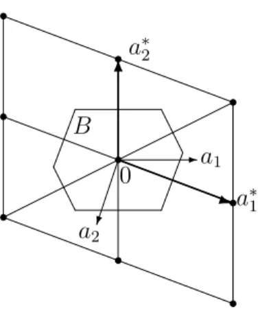
4. The Wigner-Seitz cell of the reciprocal lattice is called the (first) Brillouin zone(see Figure 1 for a two-dimensional example).

We give some explanations of the above definitions. What is the meaning of the reciprocal lattice? The reciprocal lattice vectors and the direct lattice vectors can be seen as conjugate variables, like time and frequency are conjugate variables in signal analysis. In fact, let x∈L and k∈L^∗ be given by

x= X3 m=1

αmam and k= X3 n=1

βna^∗_n, where αm, βn∈Z. Then, by (6),

e^ik^·^x = exp i

X3 m,n=1

2πδmnαmβn

= exp 2πi

X3 m=1

αmβm

= 1. (7)

(8)

-a₁

0 a^∗₁

a2

a^∗₂

B

q 6

Figure 1: The primitive vectors of a two-dimensional latticeL and its reciprocal latticeL^∗ and the Brillouin zone B.

As the position vectorxhas the dimension of length,k has the dimension of inverse length and therefore, k is called a wave vector. (More precisely, k is called a pseudo-wave vector;

see below.)

Physically, the reciprocal lattice appears in X-ray diffraction experiments with crystals.

It can be shown that the intensity peaks of the reflected X-rays are obtained when the change in the wave vector△k of the X-ray wave is an element of the reciprocal lattice [11, p. 404]. This allows one to determine the structure of the crystal lattice.

The primitive vectors a^∗_ℓ of the Brillouin zone inR³ can be computed from the vectors am by

a^∗_ℓ = 2π a_m×a_n a1 ·(a2×a3),

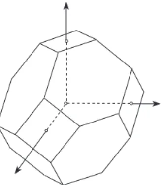
where (ℓ, m, n) is either (1,2,3), (2,3,1), or (3,1,2). Graphically, the Brillouin zone can be constructed as follows. Draw arrows from a lattice point of L^∗ to its nearest neighbors and determine the mid points of the arrows. Then the planes through these points perpendicular to the arrows form the surface of the (bounded) Brillouin zone. In two space dimensions, the Brillouin zone is a hexagon or a square (see Figure 1). In three space dimensions, the zone is a polyhedron (e.g., a “capped” octahedron; see Figure 2).

2.2 The Schr¨ odinger Equation

A semiconductor crystal consists of the nuclei, the core electrons, and the valence electrons.

Their state has to be described by quantum mechanics. More precisely, the state of a quantum particle is represented by a complex-valued wave function φ(x, t), where x∈R³ and t∈R. The dynamics of the wave function is given by the Schr¨odinger equation

i~∂tφ =Hφ, x∈R³, t >0, φ(·,0) =φI, (8)

(9)

Figure 2: Brillouin zone of semiconductors like silicon, germanium, gallium arsenide etc.

where ∂t = ∂/∂t and H is the so-called Hamilton operator. For instance, the Hamilton operator of a single electron with mass m moving in an electric potential V(x) reads as

H =−~²

2m∆−qV(x), x∈R³, (9)

where ∆ =P3

j=1∂²/∂x²_j is the Laplace operator in R³.

Stationary states can be obtained from the ansatz φ(x, t) = e⁻îEt/^~ψ(x), where E is a real number. Inserting this ansatz into (8) and dividing by e⁻îEt/^~ gives the stationary Schrödinger equation

Hψ =Eψ (10)

or, in the case of a single electron,

−~²

2m∆ψ−qV(x)ψ =Eψ, x∈R³.

Thus, the quantum state is stationary if ψ is an eigenfunction and E is an eigenvalue of H. Physically, E describes the energy of the system if it is in the eigenstate ψ. The set of all possible energy values is represented by the spectrum of the HamiltonianH (consisting not necessarily of eigenvalues only).

The solution φ of (8) with the Hamiltonian (9) can be interpreted as follows. We take the derivative

∂t|φ|² = (∂tφ)φ+φ(∂tφ) =− i~

2m∆φφ+ i~ 2mφ∆φ

=− i~

2mdiv (∇φφ−φ∇φ) =−~

mdiv Im(φ∇φ),

where z denotes the conjugate of the complex number z ∈ C, Im(z) its imaginary part, and divu =P3

j=1∂uj/∂xj is the divergence of a vector field u = (u1, u2, u3). Introducing the variables

n=|φ|², J =−q~

mIm(φ∇φ),

(10)

we arrive at the conservation law

∂_tn− 1

qdivJ = 0, expressing the conservation of the integral R

R³ndx. According to the pioneering works of Einstein, Planck etc., we may interpret n as the electron density and J as the electron current density J. The integral R

Ω|φ(x, t)|²dx is the probability to find the electron at time t in the domain Ω.

We illustrate the stationary Schr¨odinger equation and its solutions by two simple ex- amples.

Example 2.1 (State of a free electron). Consider a free electron in a one-dimensional vacuum, i.e. V(x) = 0 for all x∈R. We need to solve the Schr¨odinger equation

−~²

2mψ^′′=Eψ in R. (11)

A computation shows that eigenfunctions are given by

ψk(x) =Ae^ikx+Be⁻^ikx, x∈R, where k² = 2mE/~², with eigenvalues

E =E(k) = ~²k²

2m , k ∈R.

Thus, the eigenvalue problem (11) has infinitely many bounded solutions parametrized by k ∈ R and corresponding to different real-valued energies E(k). The functions e^±^ikx are called plane waves. Thus, the eigenstates of a free particle are plane waves.

Example 2.2 (Infinite square-well potential). We consider an electron in a square-well potential. This is a one-dimensional structure of lengthLwith a vanishing potential inside the well and an infinite potential outside. As the potential is confining the electron to the inner region, we have to solve the Schr¨odinger equation (10) in the interval (0, L) with boundary conditions

ψ(0) =ψ(L) = 0

and potential V(x) = 0 for x∈(0, L). The general solution of (10) is ψ(x) =Ae^(a+ik)x+Be⁻^(a+ik)x,

where A, B ∈ C and a and k are real numbers. Inserting this ansatz in the Schr¨odinger equation, we find that

−~²

2m(a+ ik)²ψ =Eψ,

and thus, −(a+ ik)² = 2mE/~². The boundary conditions imply that 0 =ψ(0) =A+B, 0 =ψ(L) = Ae^(a+ik)L+Be⁻^(a+ik)L.

(11)

The first equation shows thatB =−A, the second one gives e^2(a+ik)L= 1, and consequently, a= 0 and kL=nπ for all n ∈Z. Hence, the eigenfunctions are given by

ψk(x) = A(e^ikx−e⁻^ikx) =Csin(kx), where k = nπ

L , n∈Z, and C = 2iA, and the eigenvalues are

E(k) = ~²k² 2m .

The integration constant C can be determined by assuming that Z L

0 |ψk(x)|²dx= 1

holds, stating that the probability of finding the electron in the square well is equal to one.

A simple computation shows that C = √

2L. The system only allows for discrete energy states. In particular, the parameter k can take discrete values only.

2.3 Electrons in a Periodic Potential

The semiconductor solid can be described by ions (nuclei and core electrons) and valence electrons. These electrons are responsible for the electronic properties of the solid. The evolution of their state is quantum mechanically given by the Hamiltonian which takes into account the relevant physical phenomena, like ion vibrations, electron-ion interactions, and electron-electron scattering. We assume that the ions are fixed and in equilibrium such that we can neglect lattice vibrations and their interaction with the electrons (see [6, 44]

for lattice dynamics and electron-phonon interactions).

Let the state of the ion-electron system be described by the wave function ψ(x), where x= (x1, . . . , xM) ∈R^3M is the vector of all possible positions xj ∈R³ of theM electrons.

Then, the Hamiltonian of the quantum system (see Section 2.2) consists of the kinetic- energy part, the electron-ion interactions, and the electron-electron interactions,

H=−~² 2m

XM j=1

∆j +Hei+Hee,

where ∆j is the Laplace operator acting on the xj-variable only. In the following, we will derive explicit expressions for Hei and Hee:

• The lattice ions generate a periodic electrostatic potential Vei, Vei(x+y) =Vei(x) for x∈R³, y∈L,

where L describes the lattice points (nuclei), which is the superposition of the Coulomb potentials

Vj(x) = Q 4πε0|x−Rj|

(12)

of the crystal ions located at Rj, i.e.

Vei(x) =

Mi

X

j=1

Q

4πε0|x−Rj|, x∈R³

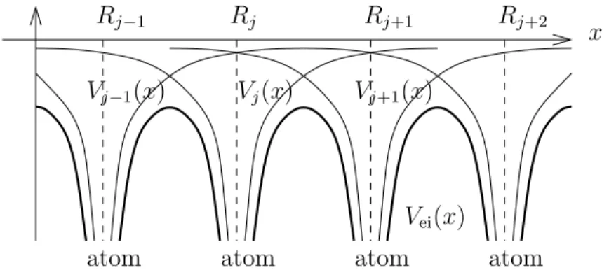
(see Figure 3). Here, Q is the ion charge, ε0 the permittivity, and Mi the number of ions. The lattice potential describes the interaction of a single electron with the ions. It is periodic with respect to the lattice. Hence, the electron-ion Hamiltonian is given by

H_ei =−q XM

ℓ=1

V_ei(x_ℓ) =− XM

ℓ=1 Mi

X

j=1

qQ 4πε0|xℓ−Rj|.

• The electron-electron interactions are modeled by V_ee(x) =−1

2 XM j,ℓ=1, j6=ℓ

q

4πε0|xj−xℓ|, x∈R^3M,

and the Hamiltonian is given by Hee = −qVee(x). The factor ¹₂ takes into account that the sum counts each interaction twice.

x Vj−1(x)

Vei(x) Vj(x) Vj+1(x)

Rj−1 Rj Rj+1 Rj+2

atom atom atom atom

Figure 3: Potentials V_j(x) of a single ion at x = R_j and net potential V_ei(x) of a one- dimensional crystal lattice.

Thus, the Hamiltonian of the system reads as H =

XM j=1

− ~²

2m∆j −qVei(xj)

−qVee(x).

The solution of the eigenvalue problem Hψ =Eψ is computationally very expensive, due to the presence of the potentials and the large number of electrons. In the following, we simplify the problem by making two approximations. First, we replace the electron-electron

(13)

interactions by an effective single-particle potential. This reduces the 3M-dimensional problem to a three-dimensional one (Hartree-Fock approximation). Second, the solution of the Schr¨odinger equation in the whole spaceR³ is reduced to the solution in a primitive cell of the lattice (Bloch decomposition).

Hartree-Fock approximation. The reduction to a single-particle potential is based on the following idea. If the electron-electron interactions can be neglected, the Schr¨odinger equation is the sum of single-particle Schr¨odinger equations. Consequently, the wave function ψ can be written as the product of the single-particle wave functions. Even in the presence of electron-electron interactions, one may try the product ansatz

ψ(x) = YM j=1

ψj(xj). (12)

This approximation of the wave function is called the Hartree approximation. The single- particle wave functions ψj are determined by assuming that they minimize the energy (ψ, Hψ)L² =R

R^3N ψHψdx under the constraint of normalized wave functions,

minψ (ψ, Hψ)_L² subject to kψjk²L² = 1 for all j, (13) where kψjk²_L² = R

R³|ψj|²dx and ψ denotes the complex conjugate of ψ. The minimum is taken over all wave functions satisfying (12).

The above approach has a drawback. By the Pauli principle, the total wave function of an electron ensemble has to be antisymmetric (with respect to the spatial and spin variables). This is not necessarily the case if the above product ansatz is employed. To overcome this limitation, we construct a properly symmetrized wave function by a linear combination of products of the type ψ1(xj1)· · ·ψN(xjN). Instead of going into the details, we only present the result and refer to [11, Ch. 7.2] for the computations. The result is the so-called Hartree–Fock equation

−~²

2m∆ψj−qVL(x)ψj =Ejψj, x∈R³, j = 1, . . . , M. (14) This is a single-particle equation in R³ incorporating the many-body aspect in terms of the total effective potential V_L. This potential is defined by V_L = V_ei+V_eff, where V_ei is the Coulomb potential defined above andVeff is the effective single-particle potential

Veff(x) =−q Z

R³

n(x^′)−n¯ex(x, x^′) 4πε0|x−x^′| dx^′,

where the electron densityn(x) and the exchange particle densitynex are given by, respectively,

n(x) = XM j=1

|ψj(x)|², nex(x, x^′) = 1 M

XM j=1

X

ℓ,k

ψj(x^′)ψℓ(x^′)ψj(x)ψℓ(x) ψj(x)ψj(x) .

(14)

The summation is over all statesℓ with parallel spin.

Bloch decomposition. In a perfect periodic crystal, we expect that the single-electron effective potential VL is periodic, too [6, p. 132]. Thus, one might hope that the whole- space Schr¨odinger problem (14) can be reduced to an eigenvalue problem on a cell of the lattice. The following result, due to Bloch [9], states that this is indeed possible.

Theorem 2.3 (Bloch). Let VL be a periodic potential, i.e., VL(x+y) = VL(x) for all x ∈R³ and y ∈ L (the Bravais lattice). Then the eigenvalue problem for the Schr¨odinger operator

H =−~²

2m∆−qVL(x), x∈R³,

can be reduced to an eigenvalue problem of the Schr¨odinger equation on the primitive cell D of the lattice, indexed by k ∈B (the Brillouin zone),

Hψ =Eψ in D, ψ(x+y) = e^ik^·^yψ(x), x∈D, y∈L. (15) For each k∈B, there exists a sequenceE_n(k), n≥1, of eigenvalues with associated eigen- functions ψn,k. The eigenvalues En(k) are real functions of k and periodic and symmetric on B. The spectrum of H is given by the union of the closed intervals{En(k) :k ∈B} for n≥1 (with B being the closure of B).

For a rigorous proof of the Bloch theorem, we refer to [42, 52], where also more properties on the energies E_n(k) are stated. In the following, we give a (mathematically not rigorous) motivation of the above statement, which helps to understand the role of the vector k.

Proof. We consider the translation operatorT_a, defined by (T_aψ)(x) =ψ(x+a) for a∈L, x∈R³, and functionsψ ∈L²(R³). First, we claim that the eigenvalues of Ta are given by e^iθ for θ ∈ R. To see this, let ψ be an eigenfunction to the eigenvalue λ, i.e. Taψ = λψ.

Then

|λ|²kψk²L² =kλψk²L² =kTaψk²L² = Z

R³

|ψ(x+a)|²dx=kψk²L², and thus, |λ|= 1 or λ= e^iθ for someθ ∈R.

The HamiltonianHcommutes with all the translation operatorsTasinceVLis periodic:

(T_aHψ)(x) =− ~²

2m∆ψ(x+a)−qV_L(x+a)ψ(x+a)

=− ~²

2m∆ψ(x+a)−qVL(x)ψ(x+a) = (HTaψ)(x).

Therefore, if ψ is an eigenfunction of H, it is also an eigenfunction of Ta for any a ∈ L and vice versa. (For this statement some mathematical properties are needed, like the self-adjointness of H and Ta; see, e.g., [5].) Letψ be such a simultaneous eigenvector ofH and Ta for any a∈L. Hence, for all j = 1,2,3, there exists θj ∈Rsuch that

T₋ajψ = e^iθ^jψ, (16)

(15)

where a1, a2, and a3 are the primitive vectors of the Bravais lattice L. We set k0 =− 1

2π X3

ℓ=1

θℓa^∗_ℓ, (17)

where a^∗₁, a^∗₂, and a^∗₃ are the primitive vectors of L^∗. Then (7) implies that k0 ·aj =− 1

2π X3

ℓ=1

θℓa^∗_ℓ ·aj =−θj. (18) We defineφ(x) = e⁻^ik⁰^·^xψ(x) forx∈R³. We claim thatφ(x+y) = φ(x) for allx∈R³ and y∈L. Since every y∈L is a linear combination of the vectors aj, it is sufficient to prove the periodicity for y=aj. We obtain, using (16) and (18),

φ(x) = e⁻îk⁰^·^xψ(x) = e⁻îk⁰^·^x(T₋_a_jψ)(x+a_j) = e⁻îk⁰^·^xeîθ^jψ(x+a_j)

= e⁻îk⁰^·^xeîθ^jeîk⁰^·^(x+a^j⁾φ(x+aj) = eî(θ^j^+k⁰^·â^j⁾φ(x+aj) = φ(x+aj).

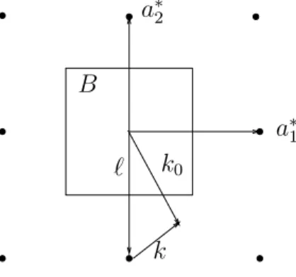
It remains to show that k0 can be restricted to the Brillouin zone. We decompose k0 = k+ℓ, where k ∈ B and ℓ ∈ L^∗ is a point in the reciprocal lattice closest to k (see Figure 4). Then

ψ(x) = eîk⁰^·^xφ(x) = eîk^·^xu(x), x∈R³, (19) where u(x) = eîℓ^·^xφ(x) satisfies, in view of (7),

u(x+y) = eîℓ^·^xeîℓ^·^yφ(x+y) = eîℓ^·^xφ(x) = u(x)

for all x∈R³ and y∈L. Now, the representation (19) implies, for x∈D and y∈L, that ψ(x+y) = e^ik^·^(x+y)u(x) = e^ik^·^yψ(x), which proves (15).

k0

ℓ B

k

a^∗₁ a^∗₂

Figure 4: Illustration of k0 =k+ℓ with k ∈B and ℓ∈L^∗.

We will often assume that the Brillouin zone can be extended to the whole space, B = R³, which is approximately satisfied for a sufficiently large number of atoms in the crystal and which can be justified by a scaling argument (see [31, Remark 1.6]).

(16)

The function k 7→En(k) is called the dispersion relation and the set {En(k) : k ∈B} the n-th energy band. It shows how the energy of then-th band depends on the (pseudo-) wave vector k. The union of ranges of En over n ∈ N is not necessarily the whole real line R, i.e., there may exist energiesE^∗ for which there is no number n∈N and no vector k ∈ B such that E_n(k) = E^∗. The connected components of the set of energies with this non-existence property are called energy gaps.

An energy gap separates two energy bands. The nearest energy band below the energy gap (if it is unique) is called the valence band, the nearest energy band above the energy gap is termed the conduction band(see Figure 5).

- 6

6?

Eg

E

k

valence band conduction band

Figure 5: Schematic band structure with energy gap Eg.

Now we are able to state the definition of a semiconductor: It is a solid with an energy gap whose value is positive and smaller than a few electron volt (up to about 3 or 4 eV).

In Table 1 the values of the energy gaps for some common semiconductor materials are collected.

Material Symbol Energy gap in eV

Indium arsenide InAs 0.356

Germanium Ge 0.661

Silicon Si 1.124

Gallium arsenide GaAs 1.424

Aluminium gallium arsenide Al0.3Ga0.7As 1.80

Aluminium arsenide AlAs 2.239

Gallium phosphide GaP 2.272

Cadmium sulfur CdS 2.514

Gallium nitride GaN 3.44

Table 1: Energy gaps of selected semiconductors (from [46, Appendix C]; the value for Al0.3Ga0.7As is taken from [29]).

.

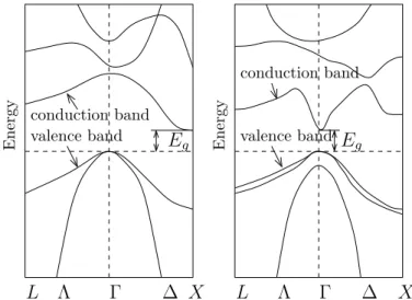
As an example, Figure 6 shows the schematic band structures of silicon and gallium arsenide. Two different crystal directions are shown, namely the k = (0,0,1)^⊤ direction

(17)

along the +k axis (called the ∆ line) and the k = (1,1,1)^⊤ direction along the −k axis (called the Λ line). The point k = (0,0,0) is termed the Γ point. The points at the boundary of the Brillouin zone in the Λ and ∆ directions are called L and X points, respectively [27, 36] (see Figure 7).

conduction band conduction band

valence band

valence band E_g E_g

L

L Λ Γ ∆ X Λ Γ ∆ X

Energy

Figure 6: Schematic band structure of silicon (left) and gallium arsenide (right) (see [49, Figs. 3.7 and 3.9]).

k_z

X

D G L

L

k_y

k_x

Figure 7: Brillouin zone of semiconductors like silicon, germanium, gallium arsenide etc.

2.4 The Semi-Classical Picture

In this section, we will motivate some equations which ressemble the classical Newton laws but which incorporate some quantum mechanical phenomena.

(18)

Semi-classical equations of motion. We will derive heuristically the following equations:

~x˙ =∇^kEn(k), ~k˙ =q∇^xV, (20) wherex is the position of the electron at timet,k is the pseudo-wave vector introduced in Section 2.3, and the dot denotes differentiation with respect to time.

First, we motivate the left equation in (20). We assume that the electrons remain for all time in the same energy band. Then we may omit the index n in ψn,k. Let ψk be a solution of the stationary Schr¨odinger equation

− ~²

2m∆ψk−q(VL(x) +V(x))ψk=En(k)ψk inD (21) with boundary conditions ψk(x+y) = e^ik^·^yψ(x), where x and y are lattice points. Recall that the momentum is represented quantum mechanically by the operator P ψ =−i~∇xψ, and its expectation value of a quantum system in the (normalized) state ψk is given by

hPik= Z

D

ψ_kP ψkdx= ~ i

Z

D

ψ_k∇xψkdx.

Then we define the mean velocity of this state by vn(k) = hPik

m .

In the semi-classical setting, we introduce a “trajectory” of the quantum system corresponding to the mean velocity by ˙x=vn(k). In this interpretation,x and k are functions of time. Employing (21), we can relate the mean velocity to the energy band.

Lemma 2.4. The semi-classical trajectory with mean velocity vn(k) is given by

˙

x=vn(k) = 1

~∇^kEn(k), t >0.

Proof. By Bloch’s Theorem 2.3, ψk can be written as

ψk(x) = e^ik^·^xuk(x). (22)

Differentiating (21) with respect tok and using ∇kψk = e^ik^·^x∇kuk+ ixψk gives (∇^kEn)ψk =− ~²

2m∆x e^ik^·^x∇^kuk+ ixψk

−(qVL+qV +En) e^ik^·^x∇^kuk+ ixψk

=

− ~²

2m∆x−(qVL+qV +En)

e^ik^·^x∇^kuk

− i~² m ∇^xψk

+ ix

− ~²

2m∆x−(qVL+qV +En) ψk.

(19)

Observing that the last term vanishes in view of (21), multiplication of the above equation with ψ_k and integration over Dyields

∇^kEn

Z

D|ψk|²dx+ i~² m

Z

D

ψ_k∇^xψkdx

= Z

D

ψ_k

− ~²

e^ik^·^x∇kuk

dx

= Z

D

e^ik^·^x∇^kuk

− ~²

ψ_kdx= 0,

where we have used integration by parts and again (21). The boundary integral in the integration-by-parts formula vanishes since uk is periodic onD. Thus, if ψk is normalized,

∇kEn= ~² im

Z

D

ψ_k∇xψkdx= ~

mhPik =~vn(k).

This shows the lemma.

The second equation in (20) is more difficult to justify (see [6, p. 220] or [36, p. 39]).

If we suppose that the total energy, consisting of the band energyEn(k) and the potential energy −qV(x), is constant along the trajectories x = x(t), k = k(t), its derivative with respect to time vanishes,

0 = d

dt(En(k)−qV(x)) =∇^kEn(k)·k˙ −q∇^xV(x)·x˙ =vn(k)·(~k˙ −q∇^xV(x)). (23) This identity is satisfied if ~k˙ −q∇^xV = 0, which is the second equation in (20). Clearly, this equation is not necessary for the energy to be conserved since (23) only shows that

~k˙ −q∇xV is perpendicular to the velocityvn(k).

Remark 2.5. The semi-classical equations (20) can be justified rigorously. The starting point is the scaled Schr¨odinger equation

ih0∂tψ =−h²₀

2 ∆ψ− h²₀ ε²VL

x ε

ψ−V(x)ψ, x∈R³,

where h0 > 0 and ε > 0. The combined classical and homogenization limit h0 → 0 and ε0 →0 is called the semi-classical limit. Here, the limitsh0 →0 and ε→0 are performed in such a way that the resulting semi-classical equation still contains quantum mechanical effects. Bechouche et al. [7] proved that the unscaled semi-classical equations of motion equal, in the limit ε=h0 →0, (20). The idea of the proof is to formulate the Schr¨odinger equation by means of the so-called Wigner function (see Section 6.2) and to perform the limit in the Wigner equation, leading to a semi-classical Vlasov equation.

Effective mass tensor. The mean velocityvn is defined byhPi^k =mvn. Employing the crystal momentum p instead of the physical momentum hPik, we may define p = m^∗vn,

(20)

where m^∗ is another mass. In the case of a free electron motion (see Example 2.1), the mass m^∗ is the rest mass of the electron since E(k) = ~²|k|²/2m yields ~k =p=m^∗v_n = m^∗∇^kE/~=m^∗~k/m and hence m^∗ =m. What is the meaning of m^∗ in the presence of a periodic potential? We differentiate the momentum p=m^∗vn with respect to time and employ the first equation in (20),

˙

p=m^∗v˙n = m^∗

~ d²En

dk² k˙ = m^∗

~² d²En

dk² p,˙ which shows that

(m^∗)⁻¹ = 1

~² d²En

dk² . (24)

This equation is considered as a definition of the effective mass m^∗. The right-hand side of this definition is the Hessian matrix of En, so the symbol (m^∗)⁻¹ is a 3×3 matrix.

The effective mass has the advantage that under some conditions, the behavior of the electrons in a crystal can be described similarly as that of a free electron gas. In order to see this, we evaluate the Hessian ofEn near a local minimum (of the conduction band), i.e.

∇kEn(k0) = 0. Then d²En(k0)/dk² is a symmetric positive definite matrix which can be diagonalized and the diagonal matrix has positive entries. We assume that the coordinates are chosen such that d²En(k0)/dk² is already diagonal,

1

~² d²En

dk² (k0) =





1/m^∗₁ 0 0

0 1/m^∗₂ 0 0 0 1/m^∗₃



.

Assume that the energy values are shifted in such a way thatEn(k0) = 0. (This is possible by fixing a reference point for the energy.) Let us further assume that already E_n(0) = 0, otherwise defineEen(k) = En(k+k0).If the functionk 7→En(k) is smooth, Taylor’s formula implies that

En(k) = En(0) +∇^kEn(0)·k+ 1

2k^⊤d²En

dk² (0)

k+O(|k|³)

= ~² 2

k²₁ m^∗₁ + k₂²

m^∗₂ + k₃² m^∗₃

+O(|k|³) for k →0,

where k= (k1, k2, k3)^⊤ and O(|k|³) denotes terms of order |k|³. If the effective masses are equal in all directions, i.e. m^∗ = m^∗₁ = m^∗₂ = m^∗₃, we can write, neglecting higher-order terms,

En(k) = ~²

2m^∗|k|². (25)

This relation is valid for wave vectors k sufficiently close to a local band minimum (of the conduction band). The scalar m^∗ is called here the isotropic effective mass. Comparing this expression with the dispersion relation of a free electron gas,

E(k) = ~² 2m|k|²,

(21)

we infer that the energy of an electron near a band minimum (of an isotropic semiconductor) equals the energy of a free electron in a vacuum where the electron rest massmis replaced by the effective massm^∗. Expression (25) is referred to as theparabolic band approximation.

Holes. When we consider the effective mass definition (24) near a maximum (of the valence band), we find that the Hessian of En is negative definite. This would lead to a negative effective mass. In order to obtain a positive mass, we may also change the sign for the group velocity vn since this is consistent with the definition p=m^∗vn. A reversed sign in the velocity means that the particles, under the influence of an electric field, travel in the opposite direction compared to electrons. This is the case if the particles have a positive charge. Employing a positive charge leads again to a positive effective mass. The corresponding (pseudo-) particles are called holes (or defect electrons). Physically, a hole is a vacant orbital in a valence band. Thus, the current flow in a semiconductor crystal comes from two sources: the flow of electrons in the conduction band and the flow of holes in the valence band. It is a convention to consider the motion of the valence band vacancies rather than the electrons moving from one vacant orbital to the next (see Figure 8).

t = 0 :

crystal atom electron

^ R orbital

vacancy

t >0 :^vacancy_^

electron

Figure 8: Motion of a valence band electron to a neighboring vacant orbital or, equivalently, of a hole in the inverse direction.

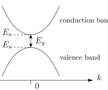
We summarize: Close to the bottom k = 0 of the conduction band in an isotropic semiconductor, the band energy becomes

En(k) = Ec+ ~²

2m^∗_e|k|², (26)

whereas near the top k = 0 of the valence band we have En(k) = Ev− ~²

2m^∗_h|k|², (27)

where Ec is the energy at the conduction band minimum, Ev the energy at the valence band maximum, m^∗_e the effective electron mass, and m^∗_h the effective hole mass. Clearly, the energy gap Eg is given byEg =Ec −Ev (see Figure 9).

2.5 Semiconductor Statistics

We will answer the question how many electrons and holes are in a semiconductor of finite size which is in thermal equilibrium (i.e. no current flow). Let f(E) be the occupation

(22)

Ec

E_v Eg

conduction band

valence band

0 k

Figure 9: Schematic conduction and valence bands near the extrema atk = 0.

density of the quantum state of energy E. We can interpret f(E) as the mean number of electrons in a quantum state of energyE =E_n(k). Then the number of electrons in a given energy band n equals the sum of all f(En(k)) over all wave vectors k. In the continuum limit the sum becomes an integral:

N_n^∗ = 2vol(Ω) (2π)^d

Z

B

f(E_n(k)) dk. (28)

The factor 2vol(Ω)/(2π)^d is called the density of states in k-space which is just a scaling factor. Here, vol(Ω) is the volume of the semiconductor, (2π)^d is related to the volume of the Brillouin zone, and the factor 2 takes into account the two possible states of the spin of an electron (see [31, Section 1.6] for details).

Electrons are fermions, i.e. particles with half-integral spin, satisfying the following properties:

1. Electrons cannot be distinguished from each other.

2. The Pauli exclusion principle holds, i.e., each quantum state can be occupied by not more than two electrons with opposite spins.

It can be shown (by maximizing the thermodynamic entropy subject to the given total number of electrons and given total energy) that the mean number of electrons in a quantum state of energy E is given by the Fermi-Dirac distribution function

f(E) = 1

1 + e^(E⁻^qµ)/k^B^T, (29)

wherekB is the Boltzmann constant (see [31, Lemma 1.11]). The two parametersT and µ are Lagrange multipliers coming from the constrained extremal problem. Thermodynamics shows that T can be interpreted as the temperature of the system and µ as the chemical potential [11, Chap. 5].

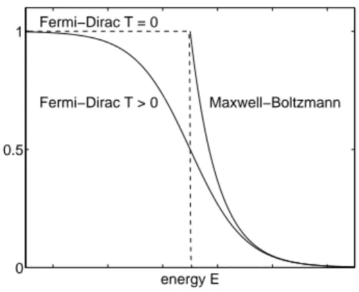
The properties of the Fermi-Dirac distribution can be understood as follows (also see [11, p. 298f.]). At zero temperature, this function becomes

f(E) =

1 for E < qµ

0 for E > qµ and f(qµ) = 1 2

(23)

(see Figure 10). This means that all states which have an energy smaller than the chemical potential are occupied, and all states with an energy larger thanqµ are empty. Physically, this behavior comes from the Pauli principle according to which two electrons must not occupy the same quantum state. At zero temperature, the states with lowest energy are filled first. The energy of the state filled by the last particle is equal to the chemical potential qµ. This number is also called the Fermi energy EF. For nonzero temperature, there is a positive probability that some energy states aboveqµ will be occupied, i.e., some particles jump to higher energy levels due to thermal excitation.

0 0.5 1

energy E Fermi−Dirac T > 0 Fermi−Dirac T = 0

Maxwell−Boltzmann

Figure 10: The Fermi-Dirac distribution at zero and nonzero temperature and the Maxwell- Boltzmann approximation.

Strictly speaking, the Fermi energy is defined as EF =qµ only if T = 0. By abuse of notation, we will also employ this terminology for T >0 (e.g., like in [27, Chap. 7.2]).

For energies much larger than the Fermi energy in the sense ofE−E_F ≫k_BT, we can approximate the Fermi-Dirac distribution by the Maxwell-Boltzmann distribution

f(E) = e⁻^(E⁻^E^F^)/k^B^T (30)

since 1/(1 + e^x)∼e⁻^x asx→ ∞ (Figure 10). Semiconductors whose electron distribution can be described by this distribution are callednondegenerate. Semiconductor materials in which the Fermi-Dirac distribution has to be used (for instance, in the case of high doping) are termed degenerate.

The electron density in a given band Ej(k) is determined by the number of electrons (28), N^∗ =N_j^∗, divided by the volume of the semiconductor domain:

n= N^∗

vol(Ω) = 2 (2π)^d

Z

B

f(Ej(k)) dk, wheref(E) = 1

1 + e^(E⁻^qµ)/k^B^T. (31) We wish to formulate the integral not in the k-space but in the energy space. For this, we introduce theDirac delta distribution δ as that functional which associates the value g(0) with an appropriate function g, i.e.δ(g) = g(0). This is also written ashδ, gi=g(0) for all

(24)

C^∞ functions g with compact support or as thesymbolic integral Z

R

δ(x)g(x) dx=g(0). (32)

We recall that this notation has to be considered with care: The symbolδ is not a function but a functional and (32) is not an integral but a symbolic representation, which is useful for the following computations.

With the Dirac distribution, the expression (31) for the electron density can be refor- mulated. We obtain from (32)

n = 2 (2π)^d

Z

B

Z

R

δ(E−Ej(k))f(E) dEdk

= Z

R

2 (2π)^d

Z

B

δ(E−Ej(k)) dk

f(E) dE.

Thus, we can write

n= Z

R

N_j(E)f(E) dE, where the integral

N_j(E) = 2 (2π)^d

Z

B

δ(E−E_j(k)) dk (33)

is called the density of states of the j-th band of energy E. In the physical literature, sometimes the notation DOS instead of N_j is used. The quantity N_j(E)△E is approximately the number of quantum states △N^∗ between E and E +△E. Thus, Nj(E) is approximately △N^∗/△E or, in the infinitesimal sense, Nj(E) = dN^∗/dE. Notice that the density of states in k-space is constant, but the density of states in energy space (33) generally is not.

Remark 2.6 (Rigorous formulation of (33)). The integral (33) can be formulated more rigourously by applying thecoarea formula, which is a curvilinear generalization of Fubini’s theorem [23]. The formula reads as follows. Let B ⊂ R^d be an appropriate domain, g : B → R be continuous, and E : B → R be continuously differentiable such that 1/|∇^kEj(k)| is integrable. Then

Z

B

g(k) dk = Z

R

Z

E_j⁻¹(e)

g(k) dSe(k)

|∇kE(k)|de, (34) where E_j⁻¹(e) = {k ∈ B : Ej(k) = e} is the level set of energy e and dSe is a surface element. Formally, by (32), this gives

N_j(E) = 2 (2π)^d

Z

R

Z

{Ej(k)=e}

δ(E−E_j(k)) dS_e(k)

|∇kEj(k)|de

= 2

(2π)^d Z

R

Z

{Ej(k)=e}

δ(E−e) dSe

|∇^kEj|de

= 2

(2π)^d Z

{Ej(k)=E}

dSE

|∇kE_j|. (35)

(25)

The density of states is thus written as a surface integral over the isoenergy surfaceE_j⁻¹(E).

We summarize these results in the following proposition.

Proposition 2.7 (Electron density). The electron density n in a given band Ej(k) reads as

n= Z

R

Nj(E)f(E) dE,

where the density of states N_j(E) at energy E is defined in (33) or (35) and the Fermi- Dirac distribution function f(E) is given in (29).

In a similar way, we can compute the density of holes in the j-th band. Taking into account that the mean number of holes in a quantum state of energy E equals the mean number of emptystates of energy E, 1−f(E), we have

p= Z

R

Nj(E)(1−f(E)) dE.

For the electron or hole density in the conduction or valence band, respectively, we write n=

Z

R

N_c(E)f(E) dE, p= Z

R

N_v(E)(1−f(E)) dE, (36) where N_c(E) and N_v(E) denote the density of states in the conduction band E_c(k) and valance band Ev(k), respectively.

If the energy band is parabolic, E(k) = E0 +~²|k|²/2, k ∈ R³, the electron and hole densities can be computed more explicitly.

Lemma 2.8 (Particle densities for parabolic bands). The three-dimensional electron and hole densities in the parabolic band and Maxwell-Boltzmann approximation qµ−E_c, E_v − qµ≪kBT are

n =Ncexpqµ−E_c kBT

, p=NvexpE_v−qµ kBT

, where Nc and Nv are the effective densities of states defined by

Nc = 2m^∗_ekBT 2π~²

3/2

, Nv = 2m^∗_hkBT 2π~²

3/2

. (37)

Proof. We start from (33), use spherical coordinates (ρ, θ, φ) and substitute z =~²ρ²/2m^∗_e to obtain

N(E) = 2 (2π)³

Z

R³