Can Lagrangian Tracking Simulate Tracer Spreading in a High-Resolution Ocean General Circulation Model?
PATRICKWAGNER, SIRENRÜHS, FRANZISKAU. SCHWARZKOPF, INGAMONIKAKOSZALKA,
ANDARNEBIASTOCH
GEOMAR Helmholtz Centre for Ocean Research Kiel, Kiel, Germany
(Manuscript received 23 July 2018, in final form 11 February 2019) ABSTRACT
To model tracer spreading in the ocean, Lagrangian simulations in an offline framework are a practical and efficient alternative to solving the advective–diffusive tracer equations online. Differences in both approaches raise the question of whether both methods are comparable. Lagrangian simulations usually use model output averaged in time, and trajectories are not subject to parameterized subgrid diffusion, which is included in the advection–diffusion equations of ocean models. Previous studies focused on diffusivity estimates in idealized models but could show that both methods yield similar results as long as the deformations-scale dynamics are resolved and a sufficient amount of Lagrangian particles is used. This study compares spreading of an Eulerian tracer simulated online and a cloud of Lagrangian particles simulated offline with velocities from the same ocean model. We use a global, eddy-resolving ocean model featuring 1/208horizontal resolution in the Agulhas region around South Africa. Tracer and particles were released at one time step in the Cape Basin and below the mixed layer and integrated for 3 years. Large-scale diagnostics, like mean pathways of floats and tracer, are almost identical and 1D horizontal distributions show no significant differences. Differences in vertical distributions, seen in a reduced vertical spreading and downward displacement of particles, are due to the combined effect of unresolved subdaily variability of the vertical velocities and the spatial variation of vertical diffusivity. This, in turn, has a small impact on the horizontal spreading behavior. The estimates of eddy diffusivity from particles and tracer yield comparable results of about 4000 m2s21in the Cape Basin.
1. Introduction
Analyses of tracer spreading are widely used in ob- servational oceanography to study subsurface ocean circulation and attendant material transport (Ledwell and Watson 1991;Ledwell et al. 1998;Ho et al. 2008;
Gary et al. 2012;Banyte et al. 2012,2013;Tulloch et al.
2014). In tracer release experiments distinct water masses are marked through conservative (i.e., remaining constant and not growing or decaying with time) and passive (i.e., not affecting the ocean flow) chemical constituents (e.g., rhodamine dye or sulfur hexa- fluoride). From subsequent measurements of the in- jected tracer concentrations, the water mass spreading (pathways), as well as mixing rates due to turbulent flows, like eddies and filaments (so-called eddy diffu- sivities), can be inferred. A common diagnostic of oceanic mixing is the calculation of a diffusivity tensor, which relates mixing rates due to turbulent flows to
the gradient of a tracer concentration. Tracer release experiments have been used to estimate the diffusivity in different regions of the world oceans (e.g., Tulloch et al. 2014;Banyte et al. 2012;Ledwell et al. 1998). Major tracer release experiments were conducted in the east- ern and northeastern Atlantic (Ledwell et al. 1998;
Sundermeyer and Price 1998;Banyte et al. 2012,2013), northeastern Pacific (Ledwell and Watson 1991; Ho et al. 2008), and Southern Oceans (Tulloch et al. 2014).
To guide and advance our understanding of ocean mixing processes, ocean general circulation models (OGCMs), often in high-resolution regional configu- rations, are a valuable tool. They help in interpreting the sparse observational spreading and diffusivity estimates, but can also be used to design tracer and float release experiments in the first place (e.g.,Banyte et al. 2013).
The OGCMs integrate a passive tracer fieldC(x,t) in time t and in the Eulerian frame (i.e., fixed spatial framexdefined on the model grid) using the advection–
diffusion equation:
Corresponding author: Patrick Wagner, pwagner@geomar.de DOI: 10.1175/JPO-D-18-0152.1
Ó2019 American Meteorological Society. For information regarding reuse of this content and general copyright information, consult theAMS Copyright Policy(www.ametsoc.org/PUBSReuseLicenses).
›C
›t 5=(KM=C)2U=(C) , (1) whereU(x,t) is the velocity andKM(x,t) is the model eddy diffusion coefficient. These, respectively, represent advection by the oceanic flow resolved by the OGCM, and the combined effect of molecular diffusion and ad- vection by unresolved turbulent flow, parameterized as Fickian diffusion (for the different formulations of the diffusivity tensorKMand numerical solution techniques;
see, e.g.,Griffies et al. 2000). The integration of Eq.(1)is usually done during the ocean model integration. Al- though popular as a diagnostic tool (e.g.,Sarmiento and Gruber 2002; Tulloch et al. 2014; Böning et al. 2016;
Dukhovskoy et al. 2016), these tracer calculations can be costly, in particular with new generations of eddy- resolving global and regional models targeting small- scale processes, and continually pushing up the limits of computational feasibility.
A practical alternative to an advective–diffusive tracer in an Eulerian framework, are Lagrangian (moving-frame, particle-following) simulations. Here, the fundamental concept of describing fluid motion as the accumulation of continuum fluid particle motion is employed. A tracer patch can be approximated by a cloud of Lagrangian particles (e.g., Sundermeyer and Price 1998;LaCasce 2008;Banyte et al. 2013). The ve- locity field of an OGCM is used to calculate a large set of individual particle trajectories, with each particle de- scribing the pathway of an imaginary point particle, that moves as a small element of fluid. Example applications of such Lagrangian studies target the spread of geo- chemical tracers (e.g., Gary et al. 2012), simulation of tracer release experiments (Banyte et al. 2013), spreading of water masses (e.g., Bower et al. 2009;
Koszalka et al. 2013;Rühs et al. 2013;Durgadoo et al.
2017), back-tracing sources of water masses (von Appen et al. 2014; Gelderloos et al. 2017), or calculation of eddy diffusivities in eddy-permitting or eddy-resolving models (Koszalka et al. 2009a;Griesel et al. 2010,2014;
Rühs et al. 2018).
The main advantages of Lagrangian techniques are lower computational costs, because the calculation is done per trajectory and not at every single model grid point. Lagrangian experiments also offer the ability to perform backward tracing and the capacity to calculate conditional statistics, like transit time distributions and water property changes, on subsets of the trajectories.
(e.g., von Appen et al. 2014; Durgadoo et al. 2017;
Gelderloos et al. 2017). Acoustically tracked Lagrangian floats (following the currents at a certain pressure or density surface) have also been used to assess lateral water mass pathways and eddy diffusivities in the
subpolar North Atlantic and in the Southern Ocean (e.g.,Zhang et al. 2001;Bower et al. 2009).
Lagrangian experiments are often done in an offline framework. The stored velocity field of an OGCM is used to advect a tracer or particles. The temporal reso- lution of the OGCM output velocity field for offline simulations can be much lower than the internal OGCM time step with which the online calculations are per- formed (e.g., Keating et al. 2011). This reduces the computational effort. Moreover, offline experiments offer a possibility of flexible use of the stored ocean model output for multiple release experiments. The Lagrangian framework does not require an offline in- tegration (e.g.,Wolfram et al. 2015) and tracer experi- ments are not limited to online calculations (e.g.,Ribbe and Tomczak 1997). Since they are commonly used we will compare these two specific setups of online Eulerian tracer and offline Lagrangian particles. This means, however, that we not only compare a Lagrangian to an Eulerian framework but also online to offline calcu- lations, and differences between our experiments can stem from either difference.
The general aim of this study is to explore if and under what assumptions do online integration of tracers and offline integration of Lagrangian particles yield similar results regarding spreading and mixing diagnostics.
Previous research addressed several aspects that could cause differences in the results.
First, offline experiments use model output sub- sampled and often averaged in time (usually daily to 5-day-mean velocities are used), which smears out short- time and small-scale advective processes simulated by the OGCM. Keating et al. (2011) examined the sensitivity to subsampling for a range of diffusivity diagnostics in two models of oceanic turbulence: the Philips model (in which tracer transport is controlled by large eddies) and the Eady model (where it is determined by local scales of motion). They defined a critical output time step criterion for the onset of ‘‘par- ticle overshoot’’ and showed that the tracer diagnostics in the Philips model show less sensitivity to the spatio- temporal subsampling as long as the deformation scale dynamics is resolved.
Second, the Eulerian tracer method in ocean model- ing has a disadvantage of being susceptible to numerical (spurious) diffusion associated with finite-element and finite-difference techniques applied to solve the advec- tion and diffusion of tracer [Eq. (1)] on a fixed grid.
These spurious effects have implications for the realism of the model solutions and pose high requirements on horizontal and vertical resolution of the model and the choice of the advection and diffusion schemes (e.g., Rood 1987; Gerdes et al. 1991; Beckers et al. 2000;
Griffies et al. 2000; Lévy et al. 2001; Delhez and Deleersnijder 2007;Spivakovskaya et al. 2007;Hill et al.
2012;Marchesiello et al. 2009; Naughten et al. 2017).
They can lead to an underestimation of spatial gradients and finescale structures (e.g., Reithmeier and Sausen 2002;Hoppe et al. 2014;Wohltmann and Rex 2009) due to an excessive transport across physical mixing barriers (Hoppe et al. 2014;McKenna et al. 2002). In the ocean, these are often associated with turbulent eddies and filaments or certain reactive processes like plankton blooms and ice formation. High initial tracer concen- trations (e.g., when simulating tracer releases) can also lead to spurious numerical advection.
In that respect, another advantage of the Lagrangian approach is that the spurious effects due to limited accuracy of numerical schemes are, in principle, elimi- nated (for analytical Lagrangian integration schemes) or greatly reduced (for the discrete Lagrangian integration schemes); for the latter method various diffusive pro- cesses can be included explicitly by virtue of carefully chosen stochastic differential equations (SDEs; see van Sebille et al. (2018) and references herein). For that reason, the Lagrangian and semi-Lagrangian methods are preferred (e.g., Abraham 1998; Koszalka et al. 2007;Spivakovskaya et al. 2007;Lehahn et al. 2017).
However, we expect the effect to act on a very small time scale in the case of eddy-permitting and eddy- resolving OGCMs.
Third, an important factor is that a sufficient number of particles is necessary to achieve robust Lagrangian statistics (Hunter et al. 1993;Davis 1994;Griffa 1996;
Spivakovskaya et al. 2007). Klocker et al. (2012a) showed that, for a given velocity field, particle- and tracer-based estimates of eddy diffusivities are equiva- lent as long as Lagrangian diffusivities are estimated from a sufficiently high number of trajectories (hun- dreds of floats) and by using their asymptotic and not their maximum values.
Even though the Lagrangian framework is frequently used in ocean modeling community, there are relatively few studies rigorously addressing the issues around its applicability. There are studies that present systematic comparisons between online tracer and offline La- grangian diffusivity estimates (e.g., Sundermeyer and Price 1998;Klocker et al. 2012a;Abernathey et al. 2013), but only for idealized models and/or velocity fields de- rived from altimetry. In general they find a good agreement between both approaches. To our knowledge nobody has ever carried out a similar comparison using a 3D primitive equation OGCM with a much richer dynamic. Moreover, a comparison between the two methods in terms of large-scale spreading diagnostics, like pathways, horizontal and vertical distributions in
function of time, and variance ellipses—relevant to a wide community of researchers dealing with water masses and basin-scale ‘‘connectivity’’—is also missing. In this work, we aim to fill this gap.
We compare the spreading of a passive tracer, in- tegrated online [Eq. (1)] in a mesoscale resolving OGCM to the dispersal of Lagrangian particles, that are advected with the stored velocities of the same OGCM.
Throughout the study we refer to the former as ‘‘tracer’’
and to the latter as ‘‘particles.’’ We address the following questions:
d Is a cloud of Lagrangian particles simulated offline capable of representing pathways of the online simu- lated tracer?
d How well do the horizontal distribution, as a function of time, agree for the two methods?
d Do particles and tracer yield consistent estimates of lateral eddy diffusivity?
To address these questions, we use an eddy-resolving OGCM configuration that resolves the greater Agulhas region with a horizontal resolution of 1/208. The scales on which this study focuses are regional to basinwide in space and intraseasonal to interannual in time. Eddies on the order of hundreds of kilometers are regarded as turbulent flow. The release experiment is conducted in the Cape Basin southeast of Africa in the South Atlantic. The region is characterized by high eddy activity and, at the same time, a lack of strong mean flow. Large anticyclonic eddies, ‘‘Agulhas rings,’’ shed from the retro- flecting Agulhas current, cross the region, while the Agulhas Current itself does not reach into the region (Lutjeharms 2006). The paper is organized as follows:
section 2describes the model and the Lagrangian soft- ware, gives an overview of the diffusivity calculations, and introduces the experimental design. Section 3 presents the results, andsection 4summarizes the results and provides a discussion.
2. Model and methods
a. Ocean general circulation model
We use a high-resolution nested model configuration of the Nucleus for European Modeling of the Ocean (NEMO) code, version 3.6 (Madec 2016), for the greater Agulhas region, called INALT20r. Embedded into a global tripolar ORCA configuration at 1/48hor- izontal resolution is a nest covering the region around southern Africa from 208W to 708E and from 508to 6.58S at 1/208resolution (;5 km), using Adaptive Grid Refinement in FORTRAN (AGRIF; Debreu et al.
2008). As the local first baroclinic Rossby radius of deformation yields about 15 km (Chelton et al. 1998),
the model setup can be regarded as mesoscale-eddy resolving (Hallberg 2013).
INALT20r is a member of a hierarchy of model con- figurations focused on the Agulhas region and is a suc- cessor of the established model configuration INALT01 (Durgadoo et al. 2013).
The vertical grid consists of 46zlevels with varying layer thickness from 6 m at the surface to 250 m in the deepest levels. Bottom topography is interpolated from 2-Minute Gridded Global Relief Data ETOPO2v21and represented by partial steps (Barnier et al. 2006). The model is forced with the CORE (version 2) forcing (Large and Yeager 2009) which builds on NCEP–NCAR reanalysis product merged with satellite-based radiation and precipitation via bulk formulas.
Laplacian and bi-Laplacian operators are used to pa- rameterize horizontal diffusion of tracer and momentum respectively. Lateral eddy diffusion coefficients are scaled with local mesh size: they are highest at the equator and decrease toward the poles. Nominal eddy coefficients for the nest are set toAth0560 m2s21(tracer, temperature, and salinity) and Amh05 263109m4s21 (momentum).
This implies that the tracer coefficients decrease from 60 m2s21 at the northern nest boundary to 40 m2s21 at the southern boundary.
The turbulent kinetic energy (TKE) model is used to estimate vertical mixing in the mixed layer (Blanke and Delecluse 1993;Gaspar et al. 1990). Background vertical mixing coefficients are set to Aty051:231025m2s21 (tracer) and Amy051:231024m2s21 (momentum). For tracer advection, the positive flux-corrected total variance dissipation (TVD) scheme is used (Zalesak 1979) which is less prone to spurious numerical dif- fusion then other available schemes (Lévy et al. 2001).
The passive tracer is simulated using the MY_TRC module of the ‘‘Tracer in the Ocean Paradigm’’ (TOP) implemented in NEMO. This provides the possibility to introduce user-defined tracer behavior. The passive tracer purely underlies advection and diffusion using the same schemes and parameters as for temperature and salinity.
For the tracer and particle release experiments de- scribed in this paper, we use a 30-yr-long integration (years 1980–2009), initialized with hydrography from the World Ocean Database (Levitus et al. 1998) and an ocean at rest, driven by interannually varying atmo- spheric boundary conditions. After a spinup phase of 20 years tracer and particles were released. The particles are advected with three-dimensional, daily mean model
velocity output. Tracer concentrations are also stored as daily averages.
We evaluate the model’s ability to represent observed mesoscale dynamics by comparing modeled and remotely sensed sea surface height (SSH) variance. Altimetric ob- servations are provided by AVISO2(Le Traon et al. 1998;
Ducet et al. 2000) (Fig. 1). The model slightly un- derestimates SSH variance, but it reproduces major fea- tures seen in the observations. The Agulhas Current, as well as the Agulhas Return Current, can be identified. The Agulhas Current retroflection is marked by a local max- imum in SSH variance. The pathways of Agulhas rings form a weak mean flow in the northwesterly direction.
Schwarzkopf et al. (2019) present a comprehensive evaluation of the INALT model family. The specific configuration used here (INATL20r) is a reduced version of the 1/208model INALT20.
b. Experimental design
The focus of this study is on the effect of mesoscale mixing on the dispersal of Eulerian tracers and La- grangian particles. The experiments were conducted in the Cape Basin, where strong mesoscale eddy activity due to the Agulhas rings coincides with the absence of strong mean currents. Those would quickly advect tracers out of the region, and thereby masking the im- pact of mesoscale processes on tracer transport and hindering statistical assessment due to exits out of the high-resolution nest. The tracer and particle release was designed such that it fulfilled the following criteria:
particles and tracer should be released in the center of this area with a sufficient horizontal distance from the coastline, the boundaries of the high-resolution nest, and the Agulhas Return Current; the initial patch should be larger than a typical Agulhas ring to ensure not all particles would be entrained by a single eddy; and the largest part of tracer and particles should stay below the mixed layer but still within the vertical extend of eddies, typically focused on the upper 1000 m (Arhan et al.
1999). The release area was therefore located at 160-m depth in a box covering 298–348S, 38–78E (marked in Fig. 1). A total of 105particles were seeded uniformly over this area. For the tracer, a layer of 10 horizontal grid boxes (0.58) was added to the release area at each side where the tracer values decay exponentially from 1 to 1/(2e) to avoid sharp gradients at the patch boundary leading to spurious numerical diffusion of the tracer. A similar transition zone is not required for the particles since they do not suffer from spurious numerical diffusion.
1http://www.ngdc.noaa.gov/mgg/global/relief/ETOPO2/ETOPO2v2-
2006/ETOPO2v2g/. 2http://www.aviso.altimetry.fr.
The particles and tracer were released on 1 January 2000. Since the year 2000 is chosen somewhat arbitrarily, sensitivity experiments were conducted to make sure that it does not represent an anomalous year in terms of particle/tracer spreading. Following the same strategy, particles were released in eight different years (1990, 1992, 1994, 1996, 1998, 2002, 2004, 2006) and advected for 2 years in each experiment. Note that a spinup phase of 10 years is already sufficient for the upper ocean dynamics. The overall size and orientation of the parti- cle patches after two years look comparable in all years, except for individual eddy tracks (not shown).
c. Lagrangian particle trajectories
For the computation of three-dimensional particle trajectories the community software ARIANE was used (Blanke and Raynaud 1997;http://stockage.univ-brest.
fr/;grima/Ariane/). ARIANE advects particles with a 3D velocity output from an OGCM. The software is well established and has been used for a range of applications concerned with diagnosis of modeled ocean circulation (Blanke et al. 1999,2001;Dutrieux et al. 2008;Pizzigalli et al. 2007; Rühs et al. 2013) and biological dispersal (e.g.,Bonhommeau et al. 2009;Scott et al. 2017).
ARIANE assumes three-dimensional nondivergence and continuity of volume to compute streamlines for successive time intervals:
›iTx1›jTy1›kTz50: (2) Here Txyz indicates the transport in the three spatial directions, andi,j, andkrefer to the three axes. Under the assumption of temporal stationarity over the sam- pling period (here 1 day), these streamlines represent true trajectories. The three velocity components are
known across each grid box interface. Each component is interpolated linearly across the grid box. Assuming the spatial extend of the grid box to be from 0 to 1 any transport componentT(r) is given by
T(r)5T(0)1r[T(1)2T(0)] , (3) withr2[0, 1]. The constraint of three-dimensional non- divergence ensures that a crossing time can be computed for at least one direction, and the shortest one defines the crossing time in the cell under consideration. The com- putation is then repeated for the next cell, with the starting position equal to the exit location from the previous cell.
We use the stored daily velocity output of the OGCM described above to calculate Lagrangian trajectories and store their position at daily intervals. Vertical velocities are diagnosed by ARIANE from the horizontal flow field. For technical reasons, particles cannot leave the high-resolution domain and are terminated upon arrival at the nest boundaries.
d. Spreading diagnostics: Time-dependent concentrations and error variance ellipses
For many diagnostics, the Lagrangian model output has to be mapped to a regular, Eulerian grid. This can be done via binning in space, that is, 2D or 3D histograms (e.g.,van Sebille et al. 2018) and the bin size has to be carefully chosen by trading the bias and the variance of the histogram estimator. An alternative is to use a Kernel estimator where the bandwidth also needs to be chosen carefully and special care has to be taken for locations close to the boundaries (e.g., Spivakovskaya et al. 2007). There are also more advanced approaches to the ‘‘pseudo-Eulerian’’ mapping, for example, via clustering (Koszalka and Lacasce 2010).
FIG. 1. SSH averaged for the period 2000–09 (contours; 20-cm interval) and SSH variance (shading; cm2; log scale) from (left) INALT20r and (right) altimetric observations (AVISO). The red box indicates the release area of the particles and the tracer, and the red line indicates the mean displacement of the particle and tracer clouds during 2 years.
We followed the approach ofGary et al. (2011). At every time step all particle positions were binned into a 0.258 3 0.258 grid with 46 vertical layers. This coarse horizontal resolution is necessary to avoid aliasing due to the reduced time step of daily data (van Sebille et al.
2018). To compare particles and tracer concentration CparticleandCtracerrespectively, the particle counts were normalized in such a way that every particle represents an equal portion of the initial tracer budget. The re- sulting concentration is further normalized with respect to the gridbox volumeV:
Cparticle(x,y,z,t)5C0 N0
H(x,y,z,t)
V(x,y,z) , (4) whereN0is the total amount of particles released,C0the initial tracer budget, andH(x,y,z,t) is the number of observed particles. This yields a concentration with dimensions m3m23 that (initially) represents the full tracer budget and can be compared to the Eulerian tracer.
Variance ellipses quantify directional spreading of tracer and particle patches. They are defined by
x l1
2
1 y
l2 2
5s, (5)
wherel1,2denotes the major and minor eigenvalues of the covariance tensor Cov(Dx,Dy) of the displacement Dx,Dy, with respect to the center of mass, and represent the standard deviation in directions of the eigenvectors y1,2. Parametersis a constant scaling factor. The angle aofy1toward thexaxis is calculated to align the axis of the ellipse with the eigenvectors:
a5arctany1(y)
y1(x). (6) The radii represent 2 times the standard deviation.
e. Estimation of lateral eddy diffusivities
The lateral eddy diffusivities derived from tracer and particles quantify the combined effect of the molecular and subgrid effects parameterized byKM in Eq. (1), and the advection by turbulent flows resolved by the OGCM, with the latter being several magnitudes larger than the former.
To estimate the dispersion of the tracer cloud, the growth of its second moment, the variance with respect to the center of mass, is estimated (Garrett 1983):
s2ij5 ð
x
ð
y
(xi2xci)(xj2xcj)C(x,y)dy dx ð
x
ð
y
C(x,y)dy dx
, (7)
whereC(x,y) is the tracer column inventory andxci is the center of mass given by
xci5 ð
x
ð
y
xiC(x,y)dy dx ð
x
ð
y
C(x,y)dy dx
, (8)
The tracer diffusivity is given by the time derivative:
ktij51 2
›s2ij
›t . (9)
The tracer statistics are computed in the domain of the high-resolution nest.
The dispersion of a Lagrangian particle in the two- dimensional case is defined as its mean quadratic excursion from its origin (Taylor 1921):
dx2ij
dt 52xi(t)dxj(t) dt 52yj(t)
ðt
0
yi(t0)dt052 ðt
0
yi(t)yj(t0)dt0 52
ðt 0
Pij(t)dt, (10)
wherexijdescribes the position vector of a particle and yij its Lagrangian velocity. The last equality does only hold if we assume a homogeneous flow field, that is, the velocity covariance Pij does only depend ont5t2t0. As above, the diffusivity is calculated as the temporal derivative of the dispersion and by averaging over all trajectories (indicated by angle brackets):
kij(t)51 2
d
dtxi(t)xj(t)
|fflfflfflfflfflfflfflfflfflfflfflfflffl{zfflfflfflfflfflfflfflfflfflfflfflfflffl}
1
5 ðt
0
Pij(t)dt
|fflfflfflfflfflfflfflfflfflfflffl{zfflfflfflfflfflfflfflfflfflfflffl}
2
. (11)
In theory, terms 1 and 2 in Eq.(11)should yield the same result, however, when applied to discrete time series, the results differ (e.g., LaCasce et al. 2014), with the first formulation being conceptually closer to the tracer- derived estimate and the latter formulation yielding smoother results, due to the convolution operator. As in LaCasce et al. (2014)we will employ both formulations to assess the methodological uncertainty.
To exclude skew fluxes we consider only the sym- metric part ofk(for a detailed discussion, seeGarrett 2006):
ksij5ksji5kij1kji
2 ; ksii5kii. (12) In general, the presence of a weak mean or large-scale (shear) flow is likely to increase the eddy diffusivity in the along shear direction. One way to deal with this
problem was suggested byOh et al. (2000). They iden- tified the cross-stream direction for every time step by decomposingkinto major and minor principal compo- nents. The minor principal component should yield a diffusivity estimate that is unaffected by the shear flow, assuming that the diffusivity is otherwise isotropic and only the along shear direction is amplified. The minor principal components can be calculated at every time step using (Brandt 1976):
ksminor5ksiisin2a2ksijsin2a1ksjjcos2a, (13) whereais the angle of the major principal axis given by
tan2a52 ksij ksii2ksjj
. (14)
For the decomposition to be possible,
ksii.0 and ksiiksjj.ksijksji. (15) Finally, another way to estimate diffusivity from La- grangian particles relies on the calculation of relative (double-particle) dispersion of particle pairs as a func- tion of time. This eliminates the effect of the mean (large-scale) flow acting pairwise on particles separated by a distancerand, by this, isolates the effects of eddy advection and/or mean or large-scale shear (e.g., LaCasce 2008;Koszalka et al. 2009b). The derivative of the relative dispersion is the relative diffusivity:
krij(t)51 2
d
dtri(t)rj(t)
, (16)
where in the diffusive limit of long time since the release, when the particles separate to large distances and their motion becomes uncorrelated, the relative diffusivity saturates to a constant value which is twice the value of absolute diffusivity.
3. Results
To compare mean pathways of tracer and particles, the center of mass of both clouds and their evolution with time will be compared. Five analyses will be pre- sented to compare the spread of tracer and particle and their spatial distributions: the spatial variance about the center of mass, the absolute horizontal extent of both clouds, the entrainment into the mixed layer, a statistical comparison of both distribution, and a check for normal distribution. Finally, diffusivities are calculated accord- ing to section 2. Most analyses will be limited to two years, because about 3% of tracer and particles has already left the high-resolution nest after 2 years
(Fig. 2). Two years is also a typical length of tracer release experiments.
a. Inventories and mean pathways
Almost identical inventories of particles and tracer in the nested region are indicating a similar mean advec- tion of both patches (Fig. 2). The comparison of the mean displacement of tracer and particles, shown in Fig. 3a) is indeed favorable. Both centers move about 1100 km in the zonal direction and 660 km in the meridional direction. The mean zonal displacement of the particles is slightly stronger when compared to the tracer, which indicates a weaker eastward dispersal.
b. Horizontal spreading
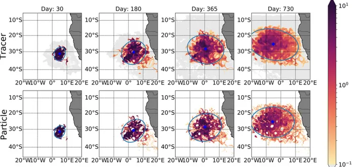
Figure 4 shows the horizontal spread of tracer and particle concentrations on a logarithmic scale at four different time steps and together with variance ellipses.
The radii represent two standard deviations while the diamonds mark the center of the clouds. The initially rectangular shapes of both patches are quickly distorted by the flow field and filaments start to evolve. Only a small amount of particles and tracer is entrained into the Agulhas retroflection zone, and quickly advected out of the Cape Basin by the Agulhas Return Current.
The turbulent stirring is mediated by eddies whose sig- natures are clearly visible in both fields.
During the first 180 days the growth of both patches is almost isotropic with respect to the center of mass, that is, the standard deviations into the major and minor direction of variance are almost equal. It is only after around 180 days that a dominant direction of dispersal is evident (Fig. 3b). The particle patch shows a much more isotropic behavior than the tracer patch; we will come back to this point below. The growth of the standard deviations in the minor variance direction are similar for both patches and only show a small offset of about 200 km after 2 years.
The area covered by tracer is larger compared to the area covered by particles (Figs. 4and3c). This is already apparent after 30 days; after 180 days the tracer has reached the western boundary of the nest at 208W, while the westernmost particle spread only to 58W. The area covered by the particles grows much slower than the area covered by tracer. After 1 year the difference amounts to 653106km2(an area of about 158 3158).
The difference is reduced by 99.8% (to 0.13106km2) if the lowest concentrations are discharged until only 99.9% of the total tracer budget is considered, and by 94% (to 3.63106km2) when 99.99% of the total tracer budget is considered. Note that the base model was used to calculate the region covered by the tracer, be- cause unlike the particles the tracer reached the nest
boundaries after 1 year. Particles are not advected across the domain, which leads to an overestimation of the discrepancies after 1 year.
Although the evolving major axes coincide with the direction of the mean displacement in northwesterly direction, that is, the direction of the mean flow (Fig. 4), the major axis of the particle cloud shows a slightly more zonal orientation which is shown in Fig. 5. This dis- crepancy is mainly due to tracer that is entrained in the Agulhas Return Current (not shown) and reduced when
all tracer concentration below the minimum particle concentrations are discharged (Fig. 5d). This reduces the total tracer budget by less than 2%.
The deepening of the mixed layer during winter has an impact on the vertical spreading, differing between tracer and particles. When wintertime mixing sets in after about 6 months after the release, the mixed layer deepens and entrains both tracer and particles (Fig. 6a).
However, the level of entrainment differs: a larger amount of tracer is entrained into the mixed layer, in
FIG. 2. Tracer (green) and particle (blue) inventories. Tracer inventory is shown separately for the base (dashed) and nested (solid) domains. Gray dashed lines indicate the limits of the analyses: 100% and day 730.
FIG. 3. (a) Mean displacements (m) of the tracer (green) and particles (blue) with respect to longitude (solid) and latitude (dashed). (b) The standard deviations (m) in the major (solid) and minor (dashed) directions of the particle cloud (blue) and the tracer patch (green).
(c) Difference of area covered by vertically integrated concentrations of the tracer and particles;
100% (blue), 99.99% (black), and 99.9% (gray) of the total tracer content are considered. Note that the global base model was used to calculate the region covered by the tracer.
particular in the second winter season (around day 600).
Ten percent of all particles are entrained in the mixed layer but almost 20% of the total tracer budget.
The reason for this varying behavior can be seen in Fig. 7, which shows the spread in zonal and vertical di- rections on a logarithmic scale. As already seen inFig. 3, low values of tracer spread much faster than particles.
This is also true for the vertical direction. The tracer fills the upper 500 m after just 30 days when particles are still confined to a depth range of 250 m around their release depth. Possible reasons are high frequency and small- scale variability of vertical velocities and/or vertical diffusion coefficient that are implicit in the online tracer simulation [Eq.(1)] but not resolved in the daily model output used to advect the particles. Once the tracer is entrained in the mixed layer, the TKE model begins to act on the tracer, providing increased vertical diffu- sivities that quickly homogenize concentrations over the vertical extend of the mixed layer.
The entrainment into the mixed layer has an impact on the vertical allocations of tracers and particles. The mean vertical displacement is shown inFig. 6b). Both centers of mass show a similar downward propagation during the first 180 days (Fig. 6) along tilted isopycnals (not shown). When the deepening of the mixed layer sets in, the tracer’s center of mass is pulled upward by almost 10 m; after day 300 it shows a continuous down- ward movement. This has an impact on the horizontal
spreading as well, because both patches are now sampled by a different horizontal velocity field. The westward velocity of the particle cloud is now stronger, while the northward component is, on average, slightly weaker, which accounts for the minor discrepancies seen in Fig. 3a). The main difference are strong absolute velocities in the mixed layer that only affect the tracer patch and increase the dispersion along the major vari- ance direction (Fig. 3b). Consequently, the time when the mixed layer deepens coincides with the time where discrepancies in the mean displacement and the spread start to evolve.
Figure 8shows the distribution of particles and tracer along the direction of minor and major variances at different time steps. To make these distributions com- parable, tracer concentrations were transformed into independent counts as follows. Each particle is assumed to represent a certain tracer volume: Vparticle5C0/N0, whereC0 is the initial tracer budget andN0 the initial number of particles. The tracer volume of every grid box was divided byVparticle to give the number of artificial tracer counts. To compare the distributions of tracer and particles a Kolmogorov–Smirnov test (e.g., Press et al. 2007) was used. The artificial tracer counts are considered independent for time scales greater than the Lagrangian decorrelation time scale of 7 days (not shown). To avoid the detection of deviations from the null hypothesis that are only due to the huge number
FIG. 4. Vertical integral of (top) tracer and (bottom) particle concentrations (m3s22; logarithmic scale) at different time steps (daily averages) after release. Variance ellipses with radii of two standard deviations are shown, and blue diamonds indicate center of mass.
of observations, but are not physically meaningful, N observations were subsampled from each dataset before the significance testing was applied. Klocker et al.
(2012b)showed that 100 floats serve as a lower boundary to gain similar lateral diffusivity estimates to these de- rived from a tracer, which is why we choose N5100.
The procedure was repeated 200 times and the averaged pvalues were considered. A close match between tracer and particle distributions is already obvious from visual inspection with the tracer distributions being slightly
broader in both directions. The discrepancies are largest at the beginning of the simulation. This is to be expected because the release strategies for both patches are dif- ferent, as descried above. Based on a significance level of 95%, no significant difference between both (tracer and particle) distributions can be detected. The distributions broaden with time but keeping a near-Gaussian shapes as confirmed by a Shapiro test (Shapiro and Wilk 1965). The tracer distribution in both directions is Gaussian shaped after 30 days. The particle distribution takes longer to adjust, but is eventually also Gaussian shaped after about 180 days (not shown). It is important to keep in mind that the initial distribution is non-Gaussian. We find that the upper and lower per mill of the tracer distribution deviate from a normal distribution (not shown).
c. Lateral eddy diffusivities
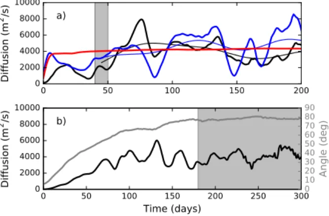
The diffusivity estimates from tracer and particles are shown inFig. 9a. Only the minor principal component, which should yield the best estimate, that is, unaffected by the mean flow (see section 2), is shown. The in- tegrated velocity covariance converges after a few days onto a value of about 4000 m2s21. To obtain a robust best estimate, the curve is averaged over the period of 40–50 days, a period greater than the integral time scale
FIG. 6. (a) Percentage of particles (blue) and tracers (green) entrained in the mixed layer. Percentage is given relative to total amount within the nested domain at the respective time step.
(b) Mean vertical displacement (m) of the tracer (green) and particles (blue).
FIG. 5. Vertical integral of tracer and particle concentrations (m3s22; logarithmic scale) at day 365 (daily average) after release for (a) the full tracer, (b) the reduced tracer with concentrations below the minimum tracer concentration discharged, and (c) the particles.
Variance ellipses are as inFig. 4. (d) The difference in major variance direction between the particles and the full tracer (solid) and between the particles and the reduced tracer (dashed).
of a few days, after which the covariance estimate con- verges and we can assume decorrelated motion. This yields 4031 m2s21. The derivative of the single-particle dispersion does not show a convergent behavior. It underestimates the former value during the first 50 days and shows strong fluctuations around the best estimate at a later stage. It is difficult to infer a robust value but
when smoothed with a window length of 91 days (thin lines inFig. 9), the derivative of the dispersion roughly converges onto the same value as the integrated velocity covariance. The estimate based on the growth of the tracers second moment, shows some resemblance to the derivative of particle dispersion. The correlation coefficient between the diffusivity series is 0.56. Again,
FIG. 7. Meridional integral of the (top) tracer and (bottom) particle concentrations (m3s22; logarithmic scale) at different time steps (daily averages). Variance ellipses with radii of two standard deviations are shown, and blue diamonds indicate the center of mass. Black line indicates mixed layer depth, averaged over the whole domain. Lines of potential density (kg m22) are also shown (blue).
FIG. 8. Distribution with respect to the center of mass along the (top) major axis and (bottom) minor axis of the variance ellipses of the particles (blue) and tracer (green) at different time steps. Dashed lines indicate the associated normal distributions.
it is difficult to infer a reliable estimate ofk, but this curve, too, oscillates around the estimate from the in- tegrated velocity covariance.
Figure 9b shows relative (i.e., double-particle) diffusion. After 10 days, the difference between zonal and meridional component is very small (not shown) indicating that the dispersion is isotropic with respect to the center of mass. The averaged separa- tion angle, shown as the gray line inFig. 9b, reaches its asymptotic value of about 808after 180 days and we will assume decorrelated motion from there on.
An average over the period 180–300 days was taken to infer a relative diffusivity estimate. The result of 4065 m2s21is in good agreement with the single- particle diffusivities.
The period after which the motion can be assumed decorrelated is very sensitive to the initial separation distance. A distance of one model grid box (about 4.7 km) was used here. When this separation scale is reduced to 1.5 km, particles show decorrelated motion only after about 300 days (not shown), still, the diffusivity, when averaged over a period when the particle motion is uncorrelated, is consistent with the nominal estimate.
Averaging the two converging measures (integrated velocity covariance and double-particle diffusion) gives an overall value of 4048 m2s21.
4. Discussion
In this work, we used a high-resolution (eddy-resolving) configuration of an OGCM to compare spreading of an Eulerian tracer simulated online and of a cloud of Lagrangian particles simulated offline with velocity output from the same model. The study domain is the greater
Agulhas region characterized by intense mesoscale vari- ability and weak mean flows.
We showed that the lateral mean displacement of tracer and particle clouds follow almost identical path- ways. This puts confidence in the estimates of mean pathways and transit times of tracer spreading that are based on particle advection (e.g.,Gary et al. 2011)—at least if particle trajectories are calculated from the daily mean output of mesoscale resolving OGCMs. We will discuss the potential sensitivity to the spatial and tem- poral resolution below.
The comparison of the spread of particle and tracer in the direction of minor variance is also favorable.
No significant differences, at the 95% level, could be detected between the 1D horizontal distributions of particles and tracers after an initial adjustment period of a few days. There is a small difference regarding the 2D horizontal distributions. Tracer seems to cover a much greater area than the particles at very low tracer concentrations (,10213m3m23). This does not yield significant differences in the overall spatial distributions between tracer and particles, because in the presented framework this extended spatial coverage after 1 year is only due to about 0.1% of the total tracer volume.
However, for the same reason, a larger amount of tracer reaches the Agulhas retroflection and accumulates in the Agulhas Return Current. This leads to a slightly different horizontal orientation of and tracer particle clouds.
These differences can only be due to parameterized or spurious numerical diffusion and numerical dispersion or due to the temporal subsampling of the velocity field used for the particles.
d Using the tracer variance equation (Klocker et al.
2012b):
1 2
›hC2i
›t 5ktotalhj=Cj2i, (17) wherektotalis the total numerical diffusivity,Cis the tracer content, and the angle brackets denote a domain average.
We find a total numerical diffusivity ofktotal5110 m2s21, which means that the spurious numerical diffusion is on the same order of magnitude as the parameterized diffusion (Ath0560 m2s21) and neither can explain the observed difference which amount to 653106km2after 1 year.
d The daily output averaged model velocities used to integrate particles do not resolve the subdaily vari- ability of the advective term (U=C) inherent in the online OGCM tracer integration [Eq. (1)]. The INALT20r model is (mesoscale) eddy resolving while
FIG. 9. Diffusivity estimates (m2s21) calculated using (a) growth of minor variance of tracer concentrations (black), growth of the particle dispersion (blue), and growth of the integral of the La- grangian velocity covariance (red) and (b) relative diffusion. Thin lines are smoothed with a 91-day Hanning window. Gray shading indicates the timespan used for averaging.
it is submesoscale permitting. The daily averages re- solve the integral time scales of 7 days and are sufficient in terms of the overshoot criterion of Keating et al.
(2011). However, while their work considered oceanic flows under quasigeostrophic approximation, our OGCM features fully three-dimensional, divergent, primitive-equation dynamics, including the vertical velocity varying on shorter time scales (inertial and shorter related to internal dynamics). The combined effect of small-scale horizontal and vertical motions leads to differences regarding the tracer and particle distributions inside eddy cores seen inFig. 4: while the particle distributions disclose the empty eddy cores (due to potential vorticity gradients at the eddy boundaries acting as mixing barriers), the tracer fields are much more smooth.
d A similar float release experiment with 53105floats showed that the volume covered by floats after 2 years already saturates at 104floats. It is therefore unlikely, that the discrepancy is due to the number of floats (here not shown).
We cannot rule out numerical dispersion as a possible reason for the discrepancies and therefore consider a combination of the latter and temporal subsampling to be the most likely reason for the small discrepancies.
There are also differences regarding the vertical dis- tributions (seeFig. 6). The average depth of the tracer after two years is about 22 m below the release depth while the particle cloud sinks about 33 m. Beside the points discussed above another possible reason is the spatial variation of numerical diffusivity:
d The spatial variation of the numerical diffusivityKzM in the tracer equation [Eq. (1)], is absent in the integration of particles. In presence of the spatially varying diffusivity, Eq.(1)yields
›C
›t 5=KM=C1KM=2C2U=C
5[=KM2U]=C1KM=2C, (18) which implies that the spatially varying diffusivity acts as an apparent velocityUk5=KM in the advection term (e.g., Hunter et al. 1993; Davis 1983, 1985). In our model, this term is negligible for the horizontal tracer diffusivity since its variation,DAth0is 20 m2s21(section 2a) over the entire nested domain. The corresponding horizontal velocity scale isUkH;20/3500,0:006 m s21, andAth0 is constant with depth. However, the vertical diffusion coefficient strongly varies with depth and time (Fig. 10) with a corresponding vertical velocity scale UZk(max);1/250;0:004 m s21, that is, ;300 m day21.
This apparent vertical velocity will lead to an effective vertical advection of tracer in the water column.The combined effect of the unresolved subdaily variability in vertical velocity, because particles are calculated offline, and the spatial variation of vertical diffusivity, which is not explicitly applied to particles, results in the greater spreading of tracer in the vertical (Fig. 7) leading to its further entrainment in the mixed layer.
Once entrained in the mixed layer, tracer is spread across the vertical extend of the mixed layer (Fig. 7), due to the increased parameterized diffusion (Fig. 10).
Spivakovskaya et al. (2007) use a Lagrangian random walk model for spatially variable vertical diffusivity to investigate the spreading of Lagrangian particles in the mixed layer with a typical vertical diffusivity profile.
They present two idealized cases for which analytic solutions are known. Given that a sufficient number of particles are used, their numerical approximation con- verges to the true value, that is, particle concentrations are mixed across the vertical extend of the domain.
Once in the mixed layer, the tracer is subject to stronger mesoscale and submesoscale variability then the particle cloud lingering below, this in turn will result in the differences in the lateral spreading seen inFig. 4.
We have shown that these differences are quite minor in terms of the inventory, mean pathways, spreading, and diffusivity diagnostics.
Are these differences relevant in the practical cases, however? It is illustrative to project our results on to a an observational tracer release. In case of the DIMES ex- periment, where a total of 75 kg of CF3SF5were injected in the ACC region (Tulloch et al. 2014), 75 g (0.1% of 75 kg) of tracer would account for the extended cover- age of the tracer. Assuming that these residual 75 g of tracer would be located in the uppermost grid box, which has the smallest possible volume, and assuming a standard density of 1024 kg m23, the resulting
FIG. 10. Spatial average over 358–158S, 108W–108E of the vertical tracer mixing parameterAty(m2s21).
concentration of 1023fmol kg21would be at least three orders of magnitude below the detection level of 0.8 fmol kg21 for the method used in the DIMES ex- periment (Ho et al. 2008). Since the discrepancy in- creases with time, the time scale under consideration is crucial. The time frame of tracer release experiments is often comparable to our simulation period (e.g., Tulloch et al. 2014).
Another argument for the consistency between the tracer and particles comes from the results concerning the lateral eddy diffusivity estimates. The estimates of diffusivity from the different methods are all in the same order of magnitude. Particle based estimates show some dependence on the method. The time derivative of the dispersion gives noisy results but the integrated velocity autocorrelation and the two-particle method yield con- sistent estimates. This is in agreement with previous studies (e.g.,Koszalka and Lacasce 2010;Klocker et al.
2012b; Griesel et al. 2014). Nevertheless, the single particle method is still valuable because it yields a metric that can be compared to its Eulerian counterpart. The resemblance of the growth of minor variance of tracer and particle patches (black and blue curves in Fig. 9) shows that the Eulerian and Lagrangian approaches yield comparable results. Our results are consistent with Klocker et al. (2012b)andWolfram and Ringler (2017), who also concluded that tracer- and particle-based es- timates should agree in general.
Finally, the obtained value for the lateral diffusivity is in agreement withRühs et al. (2018)who find surface diffusivities in the Cape Basin, estimated from drifter data and model simulations, of around 4000 m2s21. Their model configuration is similar to the one we used but provides a coarser resolution of 1/108. Based on tracer simulations and mixing length arguments,Klocker and Abernathey (2014)find lower values around 3000 m2s21. These estimates are within a typical range for open-ocean surface diffusivities.Zhurbas and Oh (2004)find values between 2000 and 7000 m2s21throughout the Pacific and Atlantic away from boundary currents and the equator.
Koszalka and Lacasce (2010) find values around 3500 m2s21in the Nordic seas. It should be kept in mind, however, that the given estimates are surface diffusiv- ities, which are likely to differ from the subsurface dif- fusivities calculated in this study.
The analysis was restricted to a certain model, thereby to a fixed resolution and conducted in an exemplary region. No sensitivity experiments with regard to reso- lution or other model specifications, like advection and diffusion schemes, were carried out here. It was shown that especially an increased vertical diffusion parameter (due to increased TKE) in the mixed layer substantially impacts the results. Therefore, it is likely that the
increased parameterization of unresolved transport in coarser models would act to increase the discrepancies between tracer and particle spread. Also, future pa- rameterization should account for observed spatial and temporal variations of diffusivity. This increased com- plexity is likely to complicate the effect of numerical tracer and particle experiments.
A more detailed investigation is needed to analyze which measures are still comparable at which degree of parameterized diffusion. Simulations of local tracer release experiments can typically utilize OGCMs that, at least in the region of interest, provide a resolution comparable to the one used here or inRühs et al. (2018).
The Cape Basin differs from other regions, as it is characterized by relatively high EKE and lacks a strong mean flow, but is otherwise indeed representative for open ocean dynamics, as the estimates for open ocean diffusivities, given above, show. On the one hand, the presented results do not suggest a different behavior of particles and tracers when introduced to a mean flow.
On the contrary, the mean displacement showed the least deviations. On the other hand, it is well known that the proportion of eddy propagation speed to mean-flow velocities are important. Diffusivities can be greatly suppressed by the mean flow when eddies propagate at a slower speed than that of the mean flow (Klocker et al.
2012a). Further work is required to assess whether these mechanisms are equally well represented by Lagrangian and Eulerian methods.
As shown above, one source of discrepancy between the spreading of tracer and particles is a strong spatial variability of the flow field, which is usually associated with strong (boundary) currents (in our case, the Agul- has retroflection). This might amplify actually small errors in the spatial distributions of particles and tracer, because both patches become entrained in different flow fields. Therefore the design of Lagrangian and tracer experiments should be done very carefully in boundary current regions.
This study compared mean advection pathways and spatial distribution of tracer and particles in a realistic OGCM for the first time and found the results of both metrics to be generally consistent, provided that the model output velocity is resolving turbulent flows that dominate the mixing, which is in agreement with Keating et al. (2011). One should take care that the relevant variability of vertical velocity and/or spatial variations of eddy diffusivity are taken into account.
The biases of the latter can in principle be estimated from the OGCM output [Eq.(18)], but because of the complexity of the fully three-dimensional dynamics, a sensitivity study to the time step could be a more practical solution.
Acknowledgments. PW was supported by the Deut- sche Forschungsgemeinschaft (DFG) as part of the Special Priority Program (SPP)-1889 ‘‘Regional Sea Level Change and Society’’ (Grant BO907/5-1). SR was supported by the Cluster of Excellence 80 ‘‘The Future Ocean’’ (Grant CP1412) within the framework of the Excellence Initiative by the DFG on behalf of the German federal and state governments. AB and FUS received funding by the German Federal Ministry of Education and Research (BMBF) for the SPACES projects AGULHAS (Grant 03F0750A) and CASISAC (Grant 03F0796A). IK received funding by the German Federal Ministry of Education and Research (BMBF) for the GROCE project (Grant 03F0778B). All model simulations have been performed at the North-German Supercomputing Alliance (HLRN).
REFERENCES
Abernathey, R., D. Ferreira, and A. Klocker, 2013: Diagnostics of isopycnal mixing in a circumpolar channel.Ocean Modell.,72, 1–16,https://doi.org/10.1016/j.ocemod.2013.07.004.
Abraham, E. R., 1998: The generation of plankton patchiness by turbulent stirring. Nature, 391, 577–580, https://doi.org/
10.1038/35361.
Arhan, M., H. Mercier, and J. R. E. Lutjeharms, 1999: The dispa- rate evolution of three Agulhas rings in the South Atlantic Ocean.J. Geophys. Res.,104, 20 987–21 005,https://doi.org/
10.1029/1998JC900047.
Banyte, D., and Coauthors, 2012: Diapycnal diffusivity at the upper boundary of the tropical North Atlantic oxygen minimum zone.J. Geophys. Res.,117, C09016,https://doi.org/10.1029/
2011JC007762.
——, M. Visbeck, T. Tanhua, T. Fischer, G. Krahmann, and J. Karstensen, 2013: Lateral diffusivity from tracer release experiments in the tropical North Atlantic thermocline.
J. Geophys. Res. Oceans, 118, 2719–2733, https://doi.org/
10.1002/jgrc.20211.
Barnier, B., and Coauthors, 2006: Impact of partial steps and mo- mentum advection schemes in a global ocean circulation model at eddy-permitting resolution.Ocean Dyn.,56, 543–
567,https://doi.org/10.1007/s10236-006-0082-1.
Beckers, J.-M., H. Burchard, E. Deleersnijder, and P. P. Mathieu, 2000: Numerical discretization of rotated diffusion operators in ocean models.Mon. Wea. Rev.,128, 2711–2733,https://
doi.org/10.1175/1520-0493(2000)128,2711:NDORDO.2.0.
CO;2.
Blanke, B., and P. Delecluse, 1993: Variability of the tropical At- lantic Ocean simulated by a general circulation model with two different mixed-layer physics. J. Phys. Oceanogr., 23, 1363–1388,https://doi.org/10.1175/1520-0485(1993)023,1363:
VOTTAO.2.0.CO;2.
——, and S. Raynaud, 1997: Kinematics of the Pacific equatorial undercurrent: An Eulerian and Lagrangian approach from GCM results. J. Phys. Oceanogr., 27, 1038–1053, https://
doi.org/10.1175/1520-0485(1997)027,1038:KOTPEU.2.0.CO;2.
——, M. Arhan, G. Madec, and S. Roche, 1999: Warm water paths in the equatorial Atlantic as diagnosed with a general circula- tion model.J. Phys. Oceanogr.,29, 2753–2768,https://doi.org/
10.1175/1520-0485(1999)029,2753:WWPITE.2.0.CO;2.
——, S. Speich, G. Madec, and K. Döös, 2001: A global diagnostic of interocean mass transfers.J. Phys. Oceanogr.,31, 1623–
1632, https://doi.org/10.1175/1520-0485(2001)031,1623:
AGDOIM.2.0.CO;2.
Bonhommeau, S., and Coauthors, 2009: Estimates of the mortality and the duration of the trans-Atlantic migration of European eel Anguilla anguillaleptocephali using a particle tracking model. J. Fish Biol., 74, 1891–1914, https://doi.org/10.1111/
j.1095-8649.2009.02298.x.
Böning, C. W., E. Behrens, A. Biastoch, K. Getzlaff, and J. L.
Bamber, 2016: Emerging impact of Greenland meltwater on deepwater formation in the North Atlantic Ocean.Nat. Geo- sci.,9, 523–527,https://doi.org/10.1038/ngeo2740.
Bower, A. S., M. S. Lozier, S. F. Gary, and C. W. Böning, 2009:
Interior pathways of the North Atlantic meridional over- turning circulation. Nature, 459, 243–247, https://doi.org/
10.1038/nature07979.
Brandt, S., 1976:Statistical and Computational Methods for Scientists and Engineers. North-Holland Publishing Company, 415 pp.
Chelton, D. B., R. A. DeSzoeke, M. G. Schlax, K. El Naggar, and N. Siwertz, 1998: Geographical variability of the first baro- clinic Rossby radius of deformation.J. Phys. Oceanogr.,28, 433–460,https://doi.org/10.1175/1520-0485(1998)028,0433:
GVOTFB.2.0.CO;2.
Davis, R. E., 1983: Oceanic property transport, Lagrangian particle statistics, and their prediction. J. Mar. Res., 41, 163–194, https://doi.org/10.1357/002224083788223018.
——, 1985: Drifter observations of coastal surface currents during CODE: The method and descriptive view.J. Geophys. Res., 90, 4741–4755,https://doi.org/10.1029/JC090iC03p04741.
——, 1994: Lagrangian and Eulerian measurements of ocean transport processes.Ocean Processes in Climate Dynamics:
Global and Mediterranean Examples, P. Malanotte-Rizzoli and A. R. Robinson, Eds., Springer, 29–60, https://doi.org/
10.1007/978-94-011-0870-6_2.
Debreu, L., C. Vouland, and E. Blayo, 2008: AGRIF: Adaptive grid refinement in Fortran.Comput. Geosci.,34, 8–13,https://
doi.org/10.1016/j.cageo.2007.01.009.
Delhez, E. J. M., and É. Deleersnijder, 2007: Overshootings and spurious oscillations caused by biharmonic mixing.Ocean Mod- ell.,17, 183–198,https://doi.org/10.1016/j.ocemod.2007.01.002.
Ducet, N., P. Y. Le Traon, and G. Reverdin, 2000: Global high- resolution mapping of ocean circulation from TOPEX/Posei- don and ERS-1 and -2.J. Geophys. Res.,105, 19 477–19 498, https://doi.org/10.1029/2000JC900063.
Dukhovskoy, D. S., and Coauthors, 2016: Greenland freshwater pathways in the sub-Arctic Seas from model experiments with passive tracers.J. Geophys. Res. Oceans,121, 877–907,https://
doi.org/10.1002/2015JC011290.
Durgadoo, J. V., B. R. Loveday, C. J. C. Reason, P. Penven, and A. Biastoch, 2013: Agulhas leakage predominantly responds to the Southern Hemisphere westerlies.J. Phys. Oceanogr.,43, 2113–2131,https://doi.org/10.1175/JPO-D-13-047.1.
——, S. Rühs, A. Biastoch, and C. W. Böning, 2017: Indian Ocean sources of Agulhas leakage. J. Geophys. Res. Oceans,122, 3481–3499,https://doi.org/10.1002/2016JC012676.
Dutrieux, P., C. E. Menkes, J. Vialard, P. Flament, and B. Blanke, 2008: Lagrangian study of tropical instability vortices in the Atlantic. J. Phys. Oceanogr., 38, 400–417, https://doi.org/
10.1175/2007JPO3763.1.
Garrett, C., 1983: On the initial streakness of a dispersing tracer in two- and three-dimensional turbulence.Dyn. Atmos. Oceans, 7, 265–277,https://doi.org/10.1016/0377-0265(83)90008-8.