High-resolution physical–biogeochemical structure of a filament and an eddy of upwelled water off northwest Africa

(1)

https://doi.org/10.5194/os-16-253-2020

High-resolution physical–biogeochemical structure of a filament and an eddy of upwelled water off northwest Africa

Wilken-Jon von Appen¹, Volker H. Strass¹, Astrid Bracher¹, Hongyan Xi¹, Cora Hörstmann¹, Morten H. Iversen¹, and Anya M. Waite²

1Alfred Wegener Institute, Helmholtz Centre for Polar and Marine Research, Am Handelshafen 12, 27570 Bremerhaven, Germany

2Department of Oceanography and the Ocean Frontier Institute, Dalhousie University, Halifax, Nova Scotia, Canada Correspondence:Wilken-Jon von Appen (wilken-jon.von.appen@awi.de)

Received: 1 October 2019 – Discussion started: 24 October 2019

Revised: 24 January 2020 – Accepted: 27 January 2020 – Published: 28 February 2020

Abstract.Nutrient-rich water upwells offshore of northwest Africa and is subsequently advected westwards. There it forms eddies and filaments with a rich spatial structure of physical and biological/biogeochemical properties. Here we present a high-resolution (2.5 km) section through upwelling filaments and an eddy obtained in May 2018 with a TRI- AXUS towed vehicle equipped with various oceanographic sensors. Physical processes at the mesoscale and submesoscale such as symmetric instability, trapping of fluid in eddies, and subduction of low potential vorticity (which we use as a water mass tracer) water can explain the observed distribution of biological production and export. We found a nitrate excess (higher concentrations of nitrate than expected from oxygen values if only influenced by production and remineralization processes) core of an anticyclonic mode water eddy. We also found a high nitrate concentration region of ≈5 km width in the mixed layer where symmetric instability appears to have injected nutrients from below into the euphotic zone. Similarly, further south high chlorophyll- a concentrations suggest that nutrients had been injected there a few days earlier. Considering that such interactions of physics and biology are ubiquitous in the upwelling regions of the world, we assume that they strongly influence the productivity of such systems and their role in CO2 uptake. The intricate interplay of different parameters at the kilometer scale needs to be taken into account when inter- preting single-profile and/or bottle data in dynamically active regions of the ocean.

1 Introduction

In the euphotic zone of a stratified ocean, productivity tends to be limited by nutrients as vertical exchange is suppressed in geostrophically balanced flows. However, dynamic processes associated with fronts may inject nutrient-rich water from below into the mixed layer, which enhances productivity (Strass, 1992) at scales that are difficult to quantify. The large upwelling systems of the world are located on the eastern side of Earth’s oceans (Chavez and Messié, 2009) such as the Mauritanian upwelling system offshore of northwest Africa. There the wind stress is such (northerly in the North- ern Hemisphere) that cold nutrient-rich water from the depths is upwelled to the surface at the coast, resulting in high productivity. In eastern boundary upwelling systems (EBUSs), the upwelled water near the coast is separated by a sharp front from the often nutrient-depleted water offshore (Capet et al., 2008a). This front is typically baroclinically unstable and can form eddies as well as mesoscale filaments, which may ef- ficiently transport upwelled water offshore for hundreds of kilometers (Hosegood et al., 2017). This detachment of filaments is often related to topographic features along the coast line (Meunier et al., 2012).

At geostrophically balanced (i.e., low Rossby number, meaning that the horizontal scales of motion are so large that Earth’s rotation is dominant in the force balance) mesoscale filaments, cross-front exchange is weak and prohibits the resupply of nutrients to the euphotic zone in the filaments.

As a result, new production in a mesoscale upwelling filament is limited as it depends on the initial injection of nutri-

(2)

ents during the upwelling process (Hosegood et al., 2017).

For larger Rossby numbers (i.e., approaching 1), the pure 2-D geostrophic balance breaks down and 3-D flows arise that contain a significant ageostrophic component which can lead to cross-front fluxes of, e.g., water, mass, and nutrients.

This submesoscale flow regime can involve vertical velocities on the order of 100 m d⁻¹. This ostensibly supplies nutrients to the mixed layer at fronts (Lévy et al., 2001, 2012) and filaments, especially at filaments generated from EBUSs that propagate into nutrient-depleted waters located offshore (Capet et al., 2008b). Submesoscale motions can also rapidly re-stratify the upper ocean in the presence of horizontal density gradients (Mahadevan et al., 2012).

Demonstrating the importance of the nutrient resupply mechanism, Hosegood et al. (2017) found that submesoscale dynamics via vertical circulations could explain a higher level of productivity in an upwelling filament off northwest Africa than could be supported only by the initial nutrient supply during the coastal upwelling. In addition to the contin- uous input of nutrients from below the mixed layer, nitrogen regeneration may support new production in the filaments (Clark et al., 2016). Such fronts and filaments are ubiquitous over Earth’s oceans, especially in regions that have processes which generate lateral density gradients, but their overall impact on vertical nutrient supply remains understudied (Ma- hadevan, 2016).

Here we investigate a system of submesoscale filaments and a mesoscale eddy in the Cape Verde Frontal Zone between 20 and 26^◦N off the northwest African coast. There isopycnal mixing between two water masses takes place (Tomczak, 1981; Martínez-Marrero et al., 2008). These water masses are the fresher South Atlantic Central Water (SACW) defined along a line from 7.24^◦C/34.95 to 16.00^◦C/35.77 in temperature–salinity (TS) space and the saltier North At- lantic Central Water (NACW) defined along a line from 7.50^◦C/35.05 via 11.00^◦C/35.47 to 18.65^◦C/36.76 in TS space (Tomczak, 1981). The salinity contrast of the two central waters stems from the excess evaporation in the subtropical North Atlantic (NACW) while the low-salinity Antarctic Intermediate Water affects the South Atlantic (SACW).

Offshore of Mauritania, along the coast of northwest Africa, the offshore motion of the upwelled water was stud- ied in 2009 (Hosegood et al., 2017). Sea surface temperature (SST) showed that upwelling of cold and nutrient-rich water close to the coast produced a strong bloom. This water was subsequently advected offshore and formed a filament that moved out into the ocean towards the west. A number of sections across edge of the filament showed strong temperature and salinity gradients between the surface ocean and greater depth. Upward movement of water appeared to take place within the filament caused by strong horizontal velocity gradients (measured by the Rossby numberRo= ^ζ

f, where ζ =^∂v

∂x−^∂u

∂y is the relative vorticity, andf is the planetary vorticity). Potential vorticity PV≈N²(f+ζ )(whereN²is

the buoyancy frequency indicating the strength of the stratification) values of opposite sign tof in an otherwise grav- itationally stable upper ocean, i.e.,ζ /f <−1, are a neces- sary condition for symmetric instability to occur (Haine and Marshall, 1998). This instability leads to slantwise convec- tion whereby water parcels are exchanged in the vertical and horizontal at the same time. This exchange can be an efficient way to bring water from below the mixed layer into the mixed layer associated with small-scale mixed layer eddies and filaments characterized byRo&1 and outcropping isopycnals.

At such locations, Hosegood et al. (2017) found higher phytoplankton concentrations (as shown by chlorophyll-a fluorescence).

Eddies are another important oceanographic feature im- pacting vertical nutrient fluxes. They are often classified according to their rotation where cyclonic (anticyclonic) eddies are associated with upward (downward) displaced isopycnals in the eddy center compared to the surrounding water. However, there are also eddies that contain downward displaced isopycnals below upward displaced ones. As the depth interval in between creates a volume of low stratification (i.e., nearly of homogenous properties) called a “mode”, these hybrid eddies are often called anticyclonic mode water eddies (ACMEs) or intra-thermocline eddies (McWilliams, 1985; Thomas, 2008). In the eastern tropical North Atlantic ACMEs make up an estimated 9 % of all eddies (Schütte et al., 2016). Anticyclonic eddies with trapped fluid (translational velocity less than peak azimuthal velocity) are retention regions of biogeochemical properties (d’Ovidio et al., 2013). The relative vorticity associated with anticyclonic eddies modifies the propagation of near-inertial internal waves;

their energy propagates downward, and part of their energy is dissipated to vertical mixing (Kunze et al., 1995) at cer- tain depths. The dissipation region for ACMEs is below their cores (Lee and Niiler, 1998).

If frictional processes can be neglected, potential vorticity (PV) is conserved in the ocean below the mixed layer.

Wind forcing at the surface can drive PV to zero (Thomas, 2005). Therefore, upwelled water from EBUSs which has moved westward has low PV which – when subducted into eddies – results in low-stratification cores of anticyclonically rotating eddies. An anticyclonic mode water eddy that trav- eled westwards from the upwelling region to Cabo Verde some 800 km away was measured by several glider sections in 2014 (Karstensen et al., 2017). The eddy contained a lens of low-salinity water in its center and had lowered isopycnals below this lens and slightly raised isopycnals above. This lens corresponded to a maximum in nitrate and almost com- pletely depleted oxygen. Karstensen et al. (2017) suggested a mechanism whereby, as the eddy propagates, at its rim nutrients are resupplied into the mixed layer through small-scale motions. In the mixed layer those nutrients move inwards, and then the organic matter sinks down and gets remineral- ized in the core. This leads to the high nitrate concentrations in the core with a corresponding near-complete consumption

(3)

of oxygen. In other words, through the gravitational settling of organic matter, the tracers nitrate and oxygen may evolve in a way that is different from a simple anticorrelation.

Eddies may also funnel sinking organic matter on its way to the sea floor. As particles sink in an anticyclone, ageostrophic velocities associated with the eddy may deflect the particles towards the center of the eddy resulting in a so- called “wine glass shape” in the particle distribution (Waite et al., 2016).

Biological–physical coupling at the kilometer scale has rarely been observed in the ocean due to observational chal- lenges. Specifically, here we ask the question: what aspects of highly resolved observed biological structures can be ex- plained by hydrography (water masses) or physical dynamics (velocities) versus active biological processes? Here we present a high-resolution section through a filament and an eddy of upwelled water offshore of northwest Africa that reveals many of the above-discussed processes in a hitherto unavailable detail. In Sect. 2 we describe the data used. Sec- tion 3 then presents (in this order) physical, biogeochemical, and biological results and discusses them. Our conclusions are in Sect. 4.

2 Data

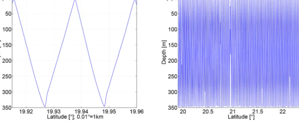
We used a MacArtney TRIAXUS E (extended version) towed undulating system which was towed at≈8 knots be- hind RV Polarstern. The TRIAXUS flew a so-called sawtooth pattern (Fig. 1a) and was slightly deflected to the side by yaw flaps so as not to measure in the wake of the ship.

Here we occupied a north-northeastward track (Fig. 2). The vehicle moved from 3 to 4 m below the surface to 350 m before coming back up to 3–4 m. At ≈1 m s⁻¹ vertical and 8 knots≈4 m s⁻¹horizontal speeds this results in a≈2.5 km distance between consecutive downcasts. Using both down- and upcasts, one could in principle get an even higher – though nonconstant – horizontal resolution. Over the total section distance of 278 km, 110 down- and upcasts were performed (Fig. 1b) resulting in a very dense (less than the first baroclinic Rossby radius of≈45 km in the region; Chelton et al., 1998) spatial coverage. The section was occupied between 30 May 17:30 and 31 May 2018 16:00 UTC. It was part of RVPolarsterncruise PS113 (Strass, 2018) that went from Chile to Germany; an overview of the encountered oceanography is given in Leach et al. (2020). As described below, in addition to the TRIAXUS, we also used vessel- mounted sensor data, analyzed underway samples, and interpreted satellite data.

2.1 TRIAXUS

The TRIAXUS is 1.95 m wide, 1.25 m tall, and 1.85 m long, and in the configuration used it had a SeaBird SBE911+

with dual temperature and conductivity sensors and the fol-

lowing auxiliary sensors: an SBE43 dissolved oxygen sensor, an SBE18 pH sensor, a WETLabs C-Star transmis- someter, a WETLabs WETStar environmental characteriza- tion optics (ECO) fluorometer, and a Satlantic photosynthetically available radiation (PAR) sensor. Furthermore, the TRI- AXUS contained a Satlantic Deep SUNA nitrate sensor and a TriOS RAMSES hyperspectral irradiance sensor. The sensor metadata are available at https://hdl.handle.net/10013/

sensor.5c126f5b-86de-469c-adf7-251789e54362 (last access: 25 February 2020), and the repository of the raw data is von Appen et al. (2019).

The SBE911+ and the auxiliary sensor data were processed using standard SeaBird routines. The deviation between the two temperature–conductivity pairs was monitored throughout the cruise, and no events of changing differences were detected. The fluorescence from the ECO fluorometer was converted to chlorophyll-a concentrations using the factory values without any further in situ calibrations. Attenuation was calculated as −1/(0.25 m)×log 10((transmissivity− 2.5 %)/100 %), where 100 %–2.5 %=97.5 % corresponded to the maximum transmissivity at depth (>250 m) which we presume to be a sensor offset.

The Deep SUNA was processed using SeaBird UCI version 1.2.1 in temperature/salinity (which were taken from the CTD – conductivity, temperature, and depth – device) correction mode. At sea, nitrate standard solutions of 7 and 14 µmol L⁻¹nitrate were used to obtain calibration point values. For this purpose, the nitrate standard of Merck Milli- pore article no. 1.19811.0500 was diluted accordingly with water and 35 g L⁻¹NaCl and 0.5 g L⁻¹NaHCO3. From the combination of these, the manufacturer suggests that one can achieve accuracies better than 2 µmol L⁻¹. A comparison with underway samples and CTD bottle calibration samples showed that they are in excellent qualitative agreement, and a correction value of minus 1 µmol L⁻¹ was determined. Especially where the samples showed values below 0.15 µmol L⁻¹ (21.5–22.5^◦N), the sensor showed very constant values around 1 µmol L⁻¹. We therefore subtracted 1 µmol L⁻¹from the sensor values and set the few values below 0 µmol L⁻¹to zero given that negative concentrations are not possible.

Near the upper and lower turning points of the sawtooth pattern (see Fig. 1), the vertical property gradients in the ocean are traversed in opposite directions (upwards and downwards) within short periods of time. Since the gradients (at least on average) will not have changed over that time pe- riod, the upcast and downcast data should be identical. For temperature, this is roughly the case, but for other sensors it is not due to their sensor lag. Attempting to shift the sensor data in time with respect to temperature such that the gradients, on average, become identical allows for a determination of the sensor lag. For oxygen we determined a sensor lag with respect to the temperature sensor of 2.5 s, and for nitrate we determined a lag with respect to the temperature sensor

(4)

Figure 1.Sawtooth pattern of observations:(a)shows an exemplary subset of the down- and upcasts and(b)shows all 110 used undulations of the section from 30 May 17:30 to 31 May 2018 16:00 UTC. The distance between consecutive downcasts is≈2.5 km.

of 20 s (though this may also be partially due to the separate data acquisition hardware of the nitrate sensor). Both sensor lags were corrected for. To further reduce inconsistencies from sensor lags, we only used data from downcasts, thereby reducing our horizontal resolution to≈2.5 km.

During the cruise, the traditional CTD rosette (Strass, 2019) was also deployed on average once a day. For the section presented here, the CTD rosette was deployed immediately before deployment and immediately after recovery of the TRIAXUS. Water samples from six depths were analyzed for inorganic nutrients (except for ammonium) (see below).

We compared the properties measured by the rosette CTD and the TRIAXUS CTD in physical and TS space and did not detect systematic deviations. Furthermore, we emphasize that our goal here was not to describe highly accurate deep ocean parameters but rather to determine relative differences in oceanic parameters in the highly variable upper 350 m of the water column. This therefore does not require as much calibration effort as would typically be done for full ocean depth CTD rosette casts.

Hyperspectral downwelling irradiance Ed(λ, z) at wave- length λ from 320 to 950 nm with an optical resolution of 3.3 nm and a spectral accuracy of 0.3 nm at depth z, down to the maximum light depth (mostly.0.1 % of surface light), was measured by two identical irradiance radiometers (RAMSES ACC-2-VIS, TriOS GmbH, Germany). One was installed on a frame and lowered off the side of the ship before the CTD stations, and the other one was installed on the TRIAXUS system. E_d(λ, z)data were further processed to the mean spectral diffuse attenuation coefficient for the upper 30 m, kd,mean(λ), including incident sunlight correction and correction for surface water waves following Mueller et al. (2003) and Stramski et al. (2008), as detailed in Tay- lor et al. (2011). To obtain the chlorophyll-a of seven major phytoplankton groups (diatoms, dinoflagellates, haptophytes, Prochlorococcus, cyanobacteria excludingProchlorococcus, chlorophytes, and chrysophytes) within the upper 30 m from the radiometry data, we followed the method of Bracher et al.

(2015). Instead of using spectral remote sensing reflectance as in Bracher et al. (2015), we applied the empirical orthogonal function (EOF) analysis to ourkd,mean(λ)dataset. Subse- quently we developed multiple linear regression models with the high-pressure liquid chromatography (HPLC) pigment- based (see underway samples subsection below) phytoplankton group chlorophyll-a(instead of using the phytoplankton pigment concentrations as in Bracher et al., 2015) as the re- sponse variable and EOF loadings as predictor variables. The model to predict seven phytoplankton groups was relatively robust. More details on the data processing, model construc- tion and cross-validation results can be found in Bracher et al.

(2020). Due to the passive nature of the sensor, the analysis is only available during daytime. Here we only focus on the average over the top 30 m of the water column; vertical pro- files of the phytoplankton groups along the sawtooth pattern of our section are presented in Bracher et al. (2020).

In addition to the setup used here, the TRIAXUS contains a 1200 kHz upward-looking and 1200 kHz downward- looking acoustic Doppler current profiler (ADCP) for the estimation of turbulence and the ocean currents at higher vertical resolution as well as an EK80 echo sounder for the estimation of zooplankton and fish biomass. With a Gaps ultra- short baseline positioning system its position can be tracked exactly. Furthermore, the TRIAXUS contains a WETLabs ac-s spectral absorption and attenuation sensor which will allow in the future for phytoplankton group determination also during nighttime.

Laplacian splines under tension (Smith and Wessel, 1990) were used to interpolate all the section data onto a regular grid from 0 to 350 m and 19.9 to 22.4^◦N with a grid spacing of 5 m vertically and 0.02^◦≈2.2 km horizontally.

2.2 Vessel-mounted sensors

The thermosalinograph data (Strass and Rohardt, 2019) from the water intake of RV Polarstern at 11 m depth were processed with standard methods as described in Rohardt (2018).

(5)

Furthermore, we used ocean velocity data from a Teledyne RDI Ocean Surveyor 150 kHz ADCP (VMADCP) mounted in the hull of RVPolarstern, 11 m below the surface (repository of the raw data: Witte, 2019). Using the Ocean Sur- veyor Sputum Interpreter (OSSI) software developed by GE- OMAR, it was processed to 2 min averages between 19 and 251 m depth (for an example of the use of an identically processed dataset, see von Appen et al., 2018). Mean volume backscattering strength (MVBS) was calculated from the echo intensity of the VMADCP using the method of Deines (1999). Surface currents were measured with an X- band marine radar mounted on RVPolarstern. The data acquisition and processing were done using the WaMoS II system as described in Hessner et al. (2019). The ADCP velocity (and MVBS) gridding was only done from 20 to 250 m.

Velocities in the grid closer to the surface than 20 m were added as follows: 0–10 m gridded velocities are the WaMoS velocities, 10–15 m are 2/3·WaMoS velocities + 1/3·ADCP velocities at 20 m, and 15–20 m are 1/3·WaMoS velocities + 2/3·ADCP velocities at 20 m.

2.3 Water sample data

Water samples were taken at six depths at the CTD stations prior to and after the TRIAXUS transect and continuously every 3 h (when the ship was moving) from the seawater system of the ship (Teflon tubing with a membrane pump). The CTD sampling depths varied but were chosen to represent the vertical variation in the phytoplankton distribution, contain- ing at least one sample below the chlorophyll-amaximum.

The samples for dissolved inorganic nutrient concentrations including nitrate, phosphate, and silicate were filtered through a 0.2 µm syringe filter and stored at −80^◦C while at sea. Nutrient concentrations were assayed on an Alliance Evolution III automatic analyzer, and calibrations were corrected for concentrations using certified reference material (CRM) 7602a (JAMSTEC; Japan) and MERCK STD (NIST Standard). Concentrations were calculated by means of standard colorimetric techniques (Grasshoff et al., 2009). At each sampling point duplicates of 4 L of seawater were filtered through a precombusted 0.7 µm 25 mm GF/F filter in order to assess particulate organic carbon (POC) (and particulate nitrogen – PN). Samples were snap frozen in liquid nitrogen and stored at−80^◦C while at sea. Total carbon and nitrogen elemental analyses were performed on an elemental analyzer (EUROEA3000; EuroVector, Italy).

For phytoplankton pigment analysis, immediately after sampling the water samples were filtered through Whatman GF/F filters. The filters were then shocked in liquid nitrogen and stored at−80^◦C. The soluble organic phytoplankton pigment concentrations were determined in the home laboratory using high-performance liquid chromatography (HPLC) according to the method of Barlow et al. (1997) adjusted to our temperature-controlled instruments as detailed in Taylor et al. (2011). We determined the list of pigments shown in

Table 2 of Taylor et al. (2011) and applied the method by Aiken et al. (2009).

The chlorophyll-a concentrations of the same seven major phytoplankton groups as from the radiometry were calculated based on diagnostic pigment (DP) analysis developed by Vidussi et al. (2001) where we followed Losa et al.

(2017) and then modified that according to Bracher et al.

(2020) to also derive the chlorophyll-a for Prochlorococ- cus. The chlorophyll-a ofProchlorococcussp. was directly given by the divinyl chlorophyll-a concentration. The total chlorophyll-a was determined from the sum of monovinyl- and divinyl-chlorophyll-a and chlorophyllide-a concentrations.

2.4 Satellite data

The delayed time product merged from all satellites called

“Global Ocean Gridded SSALTO/DUACS Sea Surface Height L4” (SSALTO/DUACS SSH L4) and derived variables were downloaded from http://marine.copernicus.eu (last access: 25 February 2020). We used the 1/4^◦gridded sea level anomaly (SLA) product which provides daily values where the data for each day were calculated from the along-track data within±3.5 d of the nominal date. Hence, the gridded values for consecutive days are based on partially overlapping data and are consequently not independent. We also used surface geostrophic currents calculated from the absolute dynamic topography (SLA + geoid).

The NOAA daily Optimum Interpolation Sea Surface Temperature (NOAA OI SST V2) (Reynolds et al., 2007) was downloaded from https://www.esrl.noaa.gov/psd/

data/gridded/data.noaa.oisst.v2.highres.html (last access:

25 February 2020). We used the 1/4^◦ daily optimally interpolated values merged from available infrared (cloud affected) and microwave (cloud penetrating) satellite data.

The Ocean Colour Climate Change Initiative (OC-CCI) chlorophyll-a dataset, version 3.1, of the European Space Agency (Sathyendranath et al., 2018) was downloaded from https://esa-oceancolour-cci.org (last access: 25 Febru- ary 2020). These are 8 d composites of merged sensor (MERIS, MODIS Aqua, SeaWiFS LAC and GAC, and VI- IRS) products.

3 Results and discussion 3.1 Remote sensing information

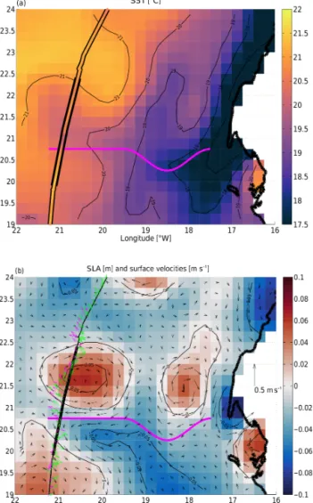
The sea surface temperature (SST) during the TRIAXUS section is shown in Fig. 2a with the cruise track around 21–22^◦W. Cold upwelled water was present near the coast.

There was also some water with colder temperatures around 21–21.5^◦N advected out from the upwelling region to the west roughly along the westward advection pathway indicated by the thick magenta line in the figure. The underway thermosalinograph data reveal similar temperatures, but the

(6)

Figure 2.Maps of satellite-based(a)sea surface temperature (in degrees Celsius; NOAA OI SST V2) and (b) sea level anomaly (in meters; SSALTO/DUACS SSH L4). Both SST and SLA are nominal from 31 May 2018, i.e., during the TRIAXUS tow. The African coast is plotted black around 17^◦W. The ship track around 21^◦W is shown in black, and in(a), data from the thermosalinograph are plotted between the black lines. The thick part of the track lines shows the towed section presented here. Panel(b)also shows geostrophic velocities (in meters per second) in black with a 0.5 m s⁻¹scale bar shown on the right over land. Green and magenta arrows plot the VMADCP/WaMoS-measured velocities in 51 and 0 m depth, respectively. The thick magenta line in both figures approximates the westward advection pathway discussed in the text.

gradients were sharper than what can be resolved with the gridded satellite data (compare also to Fig. 4a below).

The sea level anomaly (SLA) (Fig. 2b) reveals the presence of an anticyclonic eddy centered on≈20.5^◦W, 21.5^◦N.

Anticyclonic geostrophic flow encircled the sea level maximum. The shipboard measurements along the cruise track from both the VMADCP and the WaMoS radar (green and magenta in Fig. 2b) agree well with the geostrophic flow

from the satellites except for a deviation of the WaMoS velocity at the northern edge of the eddy. We refer to Hessner et al. (2019) for a more complete assessment of the differences between WaMoS and VMADCP data; they document a good qualitative and quantitative agreement for all data from the same cruise as discussed here. The thick magenta line highlights a westward advection pathway that extended from close to the coast to the cruise track between the two anticyclones (local SLA maxima) and the elongated cyclonic tongue to their south (depressed SLA). The water within that advection pathway was colder than the ambient water at the same longitude to the north or south. However, surface fluxes (such as solar warming) and possible lateral entrainment during the westward advection likely increased the temperature of the water along the pathway from much colder temperatures in the upwelling region close to the coast. Depending on the dynamics and water mass anomalies, this advection pathway could also be called a “mesoscale filament”.

Tracking of the positive sea level anomaly of the anticyclone back in time (see the Supplement) revealed that, roughly 1 month prior, the anomaly had merged from two distinct anomalies. One of those anomalies appears to have formed 2 months prior to our section at 20.5^◦W, 21.5^◦N, while the other clearly originated in the upwelling region 2.5 months prior to our section. The distance of≈360 km that it traversed in 2.5 months corresponds to a translational velocity of≈0.06 m s⁻¹. The peak azimuthal velocities of the anticyclone are≈0.5 m s⁻¹, indicating that the translational velocity is much smaller than the azimuthal velocity.

Based on this, we speculate that the anticyclone had a kine- matically trapped core which was able to transport the water in the core for great distances. During this transport the iso- lated core was subjected to biogeochemical processes (e.g., Karstensen et al., 2017).

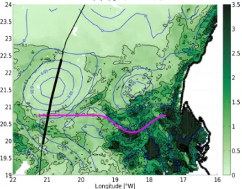
High-resolution SST and chlorophyll concentration (from ocean color) data could provide a much better synoptic view of the (sub)mesoscale features discussed in this paper. Those sensors are affected by cloud cover, and therefore no such high-resolution data are available in the study area within a few days of our 22.5 h long transect. How- ever, the average from 10 June to 17 June 2018 (Fig. 3), which is approximately 2 weeks after the TRIAXUS transect, contains sufficient information to be interpretable. The recently upwelled cold water near the coast is high in chlorophyll. The mesoscale filament providing the westward advection pathway is also associated with elevated chlorophyll concentrations. At the longitude of the transect, it has moved slightly southwards from approximately 20.9^◦N (e.g., Figs. 4b and 7d discussed below) to 20.4^◦N within the 2 weeks between the transect and the available satellite- derived chlorophyll map (Fig. 3). It is also clear that the two anticyclones (closed blue contours) are associated with very low chlorophyll concentrations.

We now turn to the section data revealing the results of these processes in the filament and eddy.

(7)

Figure 3. Map of satellite-based chlorophyll concentration (in micrograms per liter; OC-CCI v3.1 product) as color with sea level anomaly (in meters; SSALTO/DUACS SSH L4) as blue contours. The chlorophyll is an 8 d average centered on 13 June 2018 12:00 UTC, and the SLA is a 7 d average centered on 13 June 2018 00:00 UTC, i.e., approximately 2 weeks after the TRIAXUS tow.

The ship track and the westward advection pathway are plotted as in Fig. 2.

3.2 Physical properties

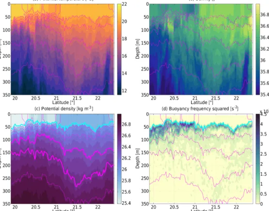
The TRIAXUS section from 19.9 to 22.4^◦N and from the surface to 350 m is shown in Fig. 4. Potential temperature (Fig. 4a) and salinity (Fig. 4b) reveal spatial structures and small-scale aspects that were resolved at much higher resolution than would have been possible with traditional CTD casts or satellite observations. These spatial structures in- clude an eddy, filaments, and mixed layer instabilities which we will present and discuss in detail below. In particular there was slightly colder water at the surface near 21^◦N which was also much fresher than the water elsewhere at the surface. That was the mesoscale filament of upwelled water which moved westward as seen (and highlighted) in the remote sensing information. The anticyclone was located to the north of the filament as will become clear below from the other parameters.

Potential density (Fig. 4c) and isopycnals (magenta lines in all section plots) reveal downward sloping isopycnals at the lower side (below≈150 m) of the anticyclone (between 21.1 and 21.9^◦N) and upward sloping isopycnals on its upper side (above≈150 m). The stratification (Fig. 4d) in the center of the anticyclone (21.5^◦N at 200 m) was slightly less than in the rest of the section at that depth, marking the mode water (region of relatively weak stratification with upward displaced isopycnals above and downward displaced isopycnals below) that the eddy was focused around. The stratification also highlights the mixed layer depth (cyan in Fig. 4c, d) which was determined from a density difference with re-

spect to the surface of 0.05 kg m⁻³. The mixed layer depth ranged from roughly 20 to 70 m, i.e., from quite shallow around 20.5^◦N to much deeper on the rim of the anticyclone (21.2 and 21.9^◦N). The density in the mixed layer within the anticyclone was significantly higher than waters further to the south. This implies the presence of a significant horizontal density gradient in the mixed layer. These sections also show that the mesoscale filament near 21^◦N corresponded to sloping isopycnals between upward doming in the south and downward displacements to the north.

A temperature–salinity plot of all measurements of the section (Fig. 5a) highlights the isopycnal mixing between North Atlantic Central Water (NACW) which is warm and salty, reminiscent of the subtropical North Atlantic, and the South Atlantic Central Water (SACW) which is fresher with its properties probably influenced by the tropical Atlantic or by Antarctic Intermediate Water (AAIW).

An isopycnal decomposition of the measured temperature and salinity (Fig. 4a, b) into SACW and NACW (as defined by the lines in Fig. 5a) shows where these water masses were located (Fig. 5b). Around 20.4^◦N the slanted front between SACW to the south and NACW to the north becomes clear, but this front had no dynamic signature given that the isopycnals were roughly flat. The anticyclone north of 21^◦N was comprised of fairly pure NACW with a concentration maximum in its mode. The strong isopycnal mixing of the Cape Verde Frontal Zone (the confluent region of NACW and SACW; see Tomczak, 1981; Martínez-Marrero et al., 2008) is evident in the large horizontal gradients over a few kilometers between 20.4 and 21.0^◦N where advected blobs of water often only occupy≈10 km and a part of the upper 350 m.

SACW was most pronounced in the mixed layer in the southern part of the section, but it also contributed roughly half to the mixed layer in the northern part of the section. A narrow band (<20 km) of SACW at depth was also present north of the anticyclone (≈22.2^◦N).

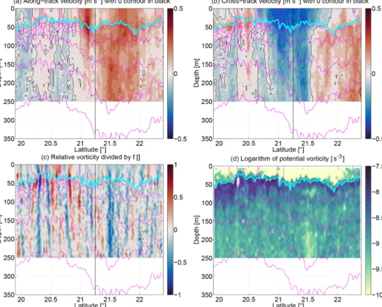
Next we will examine the dynamics starting with the velocity structure. We investigate the velocity in the direction of the cruise transect (“along-track velocity”; Fig. 6a), where positive values roughly correspond to northward velocity as well as the velocity perpendicular to the direction of the cruise transect (“cross-track velocity”; Fig. 6b), where positive values roughly correspond to eastward velocity. The ship track clearly passed through the western side of the anticyclone. Northward flow throughout most of the feature (21–

22^◦N) is observed with westward (negative cross-track) flow on its southern side (south of 21.5^◦N) and eastward flow on its northern side. This mesoscale (order of 50 km) coherent flow structure dominated the northern part of the section. In contrast, south of 21^◦N, there was a lot of variability in the velocity on smaller scales of 1–5 km.

Since we do not resolve the velocity structure in the cross- track direction, we can only estimate one component of the relative vorticityζ =^∂v

∂x−^∂u

∂y ≈ −^∂u^r

∂yr, whereu_ris the cross- track velocity, andy_r is the along-track coordinate. This esti-

(8)

Figure 4.Sections of(a)potential temperature (in degrees Celsius),(b)salinity,(c)potential density (in kilograms per cubic meter), and (d)stratification (buoyancy frequency squared) (in per second squared). In this and all the following figures, the magenta lines are isopycnals plotted at a spacing of 0.2 kg m⁻³; the 26.4 and 26.6 kg m⁻³ isopycnals are plotted as thick lines in(c). The cyan line here and below indicates the base of the mixed layer as determined from a density difference with respect to the surface of 0.05 kg m⁻³.

Figure 5. (a)Temperature–salinity diagram of all measured CTD data with the fresher South Atlantic Central Water (SACW) and the saltier North Atlantic Central Water (NACW) end-member lines according to Tomczak (1981) marked in black.(b)Section of warm, salty North Atlantic Central Water (NACW) end-member fraction for an isopycnal decomposition between SACW and NACW. The 0.5 contour is indicated in black. The mixed layer depth and isopycnals are as in Fig. 4.

mate of the relative vorticity normalized by the Coriolis fre- quencyf, i.e., the Rossby numberRo(Fig. 6c), shows strong velocity gradients at the base of the mixed layer in the southern part of the section with relative vorticities of up to±1.

Since mesoscale flows would only have |Ro| 1, and the

largeRoclearly appear to be located at the base of the mixed layer, this suggests that submesoscale mixed layer eddies or filaments were present there in association with distinct ex- trema of the NACW/SACW water mass fraction. The radius of these is 5–10 km, which is much less than the first baro-

(9)

Figure 6.Sections of(a)along-track velocity (in meters per second; positive, roughly northward),(b)cross-track velocity (in meters per second; positive, roughly eastward),(c)Rossby number (relative vorticity divided byf), and(d)logarithm of potential vorticity (in per second cubed). The vertical black line at 21.25^◦N highlights where the course of the section turned by 4^◦from 10.5 to 14.5^◦with respect to true north.

clinic Rossby radius (^N_fH) of≈45 km in the region (Chel- ton et al., 1998) and closer to the mixed layer Rossby radius (^N_f^MLH_ML), whereH andN are the full water column depth and the stratification averaged over the full depth, andH_ML andN_MLare those quantities averaged over the mixed layer.

The potential vorticity PV=N²×(f+ζ )(plotted logarith- mically in Fig. 6d) shows the effect of wind destruction of PV in the mixed layer. It also picks out the near-zero PV core of the anticyclone at 21.5^◦N at 200 m. Since PV in the ocean below the mixed layer is conserved except for mixing or other diapycnal processes, it seems that the water in the core came from a location where its PV was forced to zero, i.e., likely under wind or negative buoyancy (cooling) forcing. In other words, we can use PV as a passive tracer of the history of a water parcel. This is another piece of evidence that suggests that the mode water in the ACME originated in the upwelling region. At 20.3^◦N at 50 m (the base of the mixed layer), PV was negative (it appears white in the figure as it is outside of the range of the positive logarithmic plot). This is an indication for symmetric instability which rapidly overturns and thereby brings the system back to neu- tral levels of zero PV (marginal stability). In the process, it likely induced vertical mixing with implications for biogeo-

chemistry (discussed in more detail in Sect. 3.5 below). At 20.4^◦N it appears to also have recently injected fluid into the mixed layer as PV6=0 there (if fluid would have stayed in the mixed layer for longer, the wind would have driven its PV to zero).

3.3 Biogeochemical properties

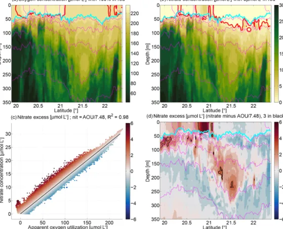
Now we turn to the observed biogeochemical structure. Oxy- gen concentrations (section in Fig. 7a; averaged over the top 20 m in Fig. 8a) and nitrate concentrations (Figs. 7b, 8a) were measured by two independent sensors with different measurement principles. Phosphate and silicate are not thought to be the limiting nutrients in this region (Bachmann et al., 2018) as is also suggested from the high phosphate and silicate concentrations detected in the underway (Fig. 8a) and CTD-rosette samples. Thus we consider nitrate as sufficient to study the nutrient availability for phytoplankton growth. In order to highlight similarities, the color axes between Fig. 7a and b are reversed as nitrate is used up and oxygen is released during primary production. Thus as long as biology remains the primary influence on the two parameters, their relation follows a roughly constant ratio, which is typical for much of the world ocean and is related to the equivalent of a Red-

(10)

Figure 7.Sections of(a)oxygen concentration (in micromoles per liter),(b)nitrate concentration (in micromoles per liter), and(d)nitrate excess (in micromoles per liter). Highlighted are the following contours:(a)100 % oxygen in red,(b)3 µmol L⁻¹nitrate in red, and (d)3 µmol L⁻¹nitrate excess in black.(c)All data in scatter plot of apparent oxygen utilization versus nitrate concentration where the black line is a best-fit linear regression, with nitrate = AOU/7.48. A nitrate excess of zero is on the black line in(c); positive/negative nitrate excess is colored red/blue above/below the black line in(c).

field ratio (Thomas, 2002; Waite et al., 2015), and reflects the biogeochemical uptake of nitrate and stoichiometric re- lease of oxygen during photosynthesis. On first sight there is a lot of agreement between oxygen and nitrate overlaid on a pronounced variability (Fig. 7a, b). Following individual isopycnals below the mixed layer, SACW was more nitrate rich/oxygen poor than NACW, suggesting that SACW may be older (having been removed from atmospheric fluxes in the mixed layer for a longer duration). The red lines in Fig. 7a indicate 100 % oxygen saturation. Apparent oxygen utilization (AOU) is the oxygen concentration at 100 % oxygen saturation (i.e., in diffusive balance with the atmosphere) as calculated from the measured temperature/salinity minus the measured oxygen concentration. The mixed layer was supersaturated (negative AOU) in places both to the north and south of the anticyclone (Fig. 8a), suggesting that primary production had supplied oxygen to the mixed layer more recently than the gas equilibration timescale. The nitrate concentration in the mixed layer in this spring/summer condition was very low (lowest underway measurement of 0.01 µmol L⁻¹at 21.6^◦N), but e.g., at 20.9^◦N there was actu- ally still a significant amount (up to 5 µmol L⁻¹) in the mixed

layer. At depth by contrast, just below 100 m, especially in the southern part, very nitrate rich values were reached (>20 µmol L⁻¹; Fig. 7b). Such concentrations, if upwelled into the euphotic zone, would have the capacity to support increased productivity.

AOU is plotted versus nitrate concentration in Fig. 7c.

Most of the individual measurements (colored dots) are close to proportional following the relation nitrate concentration

=AOU/7.48. This value is within typical observations of scatter around the Redfield ratio for organic matter (Thomas, 2002; Waite et al., 2015). However, not all individual measurements are directly proportional, and the color indicates where there is nitrate excess, e.g., for the dark red dots in the bottom left of Fig. 7c; at zero AOU, zero nitrate concentration would be expected, but in fact≈5 µmol L⁻¹(i.e., an excess of 5 µmol L⁻¹) was observed. We note that this defi- nition of nitrate excess is only based upon our measurements (Fig. 7c).

The spatial distribution of the nitrate excess (Fig. 7d) highlights the cool, fresh mesoscale filament that came from the east which still had non-zero nitrate values in the mixed layer. A significant nitrate excess is also visible in the core

(11)

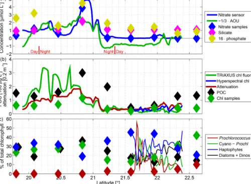
Figure 8.Mixed layer properties with sensor measurements averaged over 0–20 m in(a, b)and 0–30 m in(c)as lines and samples from 11 m as diamonds.(a)Concentrations (in micromoles per liter) of nitrate (blue),−1/3·AOU (green), silicate (magenta), and 16·phosphate.

(b)Chlorophyll-aconcentration (in micrograms per liter) from the fluorescence sensor on the TRIAXUS CTD (green line), samples (green diamonds), and the hyperspectral irradiance sensor (blue), attenuation (0.2 m⁻¹; red), and particulate organic carbon (100 µg L⁻¹; black).

Note the different units used on theyaxis.(c)Percentage of total chlorophyll-aaccounted for by different phytoplankton functional types:

Prochlorococcus(red), cyanobacteria excludingProchlorococcus(green), haptophytes (blue), and sum of diatoms and autotrophic dinoflagellates (black). Lines are from the hyperspectral irradiance sensor and diamonds are from HPLC measurements of underway samples.

of the anticyclone and in blobs in the thermocline in the south. We speculate that positive nitrate excess can originate from mixed layer water that was not equilibrated (equilibration here is understood as being where gas equilibration with the atmosphere has brought oxygen to 100 % saturation, and primary production consumed the nitrate to zero). Large undersaturation of oxygen (as is common in the upwelled water in the Mauritanian upwelling system) may have led to strong oxygen fluxes (equivalent to a reduction in AOU) from the atmosphere to the mixed layer. At the same time, the residence time in the upper ocean probably was not long enough for primary production to utilize available nitrate before the water was subducted. We hypothesize that the water in the core of the anticyclone during our section spent only a short time (∼weeks) in the mixed layer before being subducted (i.e., removed from equilibrating processes in the mixed layer) to form the anticyclone. Assuming that the correlation in Fig. 7c corresponds to the near-Redfield behavior of phytoplankton growth and remineralization in the study area, primary production and remineralization acting in a parcel of water can move it parallel to the correlation line (black line in Fig. 7c) but not change its nitrate excess (i.e., move it further away from the line). A change in the nitrate excess can only be achieved by a process that acts differently upon nitrate than upon oxygen. Gas exchange with the atmosphere likely plays

that role as it only acts upon oxygen but not upon nitrate. The gas exchange rate also depends upon how far from equilibrium with the atmosphere (100 % oxygen concentration) the parcel of water is. That is, the gas exchange rate will be faster upon the upwelling of the extremely undersaturated water, thereby pumping oxygen into the water from the atmosphere.

This corresponds to a reduction of AOU and a corresponding increase in the nitrate excess. After primary production has acted, the water may be close to saturation or slightly supersaturated. However, because the water is closer to equilibrium then, the loss of oxygen to the atmosphere will be comparatively slower. Thus a nitrate excess can be present in the mixed layer relatively soon after upwelling (as measured by the relatively slow gas exchange near equilibrium).

If the water gets subducted (stopping the gas exchange) during that time, a nitrate excess can also be observed later on.

Part of this hypothesis is that we assume that a nitrate excess of roughly zero is present in the water when it is upwelled.

This is based upon the assumption that if, in our section, we sample water that will upwell in the future, it would be “old”

(high AOU and high nitrate concentration) and would thus fall in the top right quadrant of Fig. 7c, where we observe a very small nitrate excess as defined here. In a similar sense, the filament south of 21^◦N must have been part of an offshore advection “highway” from the upwelling region whose

(12)

advective time was short enough for the above argument to hold.

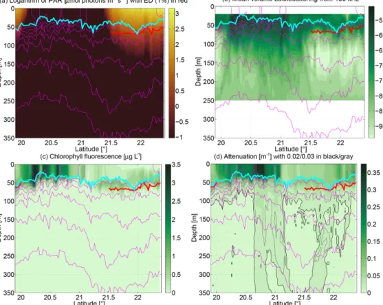
Considering the energy source for primary production, photosynthetically available radiation (PAR) as shown loga- rithmically in Fig. 9a is affected by the sunset around 20.1^◦N and the sunrise around 21.4^◦N. During the daytime, the euphotic depth (1 % level of surface PAR) as shown by the red line varied between 50 and 70 m. In the southernmost part of the section this limit for primary production coincided with the base of the mixed layer (cyan line). By contrast, in the northern part, light reached into the stratified water column below the nutrient-depleted mixed layer.

3.4 Biological properties

Phytoplankton standing stock in the water column can be inferred from chlorophyll-a fluorescence (Fig. 9c) or light attenuation (Fig. 9d) with a number of assumptions. Here we compare the chlorophyll-a fluorescence sensor that is part of the TRIAXUS CTD with the underway samples of chlorophyll-a concentration from the mixed layer (Fig. 8b).

The laboratory culture-based calibration of the fluorescence may be off by a factor of 2 due to species specific variations and environmental adaptations, and, during daytime, photochemical quenching in the upper part of the water column can diminish significantly the chlorophyll-a fluorescence signal (Falkowski and Kolber, 1995). In that situation the measured fluorescence is lower than the chlorophyll-a concentration present in the water column. This is apparent in the upper 20 m north of 21.7^◦N. Light attenuation by contrast responds to any matter in the water, but in the open ocean observed here, that is primarily phytoplankton and its degraded particulate organic matter. The chlorophyll-afluorescence from the TRIAXUS CTD may however be used to study relative changes within a region of the transect. Especially south of the anticyclone, chlorophyll-a fluorescence and attenuation were high in the mixed layer, which also corresponded to large particulate organic carbon (POC) values (Fig. 8b) to- gether with considerable spatial variability in chlorophyll-a fluorescence.

In the anticyclone, the TRIAXUS chlorophyll-a fluorescence data from the section (Fig. 9c) indicate a deep chlorophyll-amaximum at≈50–70 m in the stratified water column below the nitrate-depleted mixed layer. However, this may well be an artifact of possible quenching of chlorophyll- a fluorescence during daylight. In the southern part of the section (where measurements were taken during nighttime, and therefore chlorophyll-a fluorescence data are more robust in indicating chlorophyll-a concentration), by contrast, the values in the mixed layer were much higher. Maxima of chlorophyll-afluorescence and attenuation were observed where isopycnals were vertical in the mixed layer (Fig. 9c, d). At those locations, thermocline waters were outcropping, and horizontal density gradients in the mixed layer were present, e.g., at 20.3^◦N (chlorophyll-a fluorescence max-

imum), 20.6^◦N (attenuation maximum), and 21^◦N. These mixing processes may be responsible for the high productivity in the southern sector and will be discussed in more detail below. North of the anticyclone, light attenuation in the mixed layer and chlorophyll-afluorescence also point to fa- vorable growth conditions (this is below the depth where during daytime photochemical quenching takes place, enforcing the quality of these data). The reduction of the euphotic depth from 70 m just to the south to 50 m at 22.1^◦N correlates with the increase in attenuation, and it therefore may be the result of a higher concentration of phytoplankton and associated colored dissolved and particulate organic matter. This suggests that the euphotic depth south of the anticyclone (where we have not measured it due to nighttime) would have been shallower, thereby inhibiting growth below the mixed layer there.

In the mixed layer, oxygen (Fig. 8a) was supersaturated (negative AOU) in the southern part, and nitrate remained available with especially large excess values at 20.9^◦N. In contrast, in the northern part nitrate was low but not entirely zero, e.g., around 22.1^◦N. The attenuation correlates very well with the total chlorophyll-a concentration determined from the continuously measured spectrally resolved radiometric data via the EOF method (only available for the daytime part of our transect) and with the chlorophyll-a determined from discrete water samples via HPLC analysis. This is because in these so-called optical case-1 waters (see Morel and Prieur, 1977) the light attenuation is determined mostly by the concentration of phytoplankton pigments and related colored dissolved and the particulate organic matter. How- ever chlorophyll-a determined from the fluorescence sensor that is part of the TRIAXUS CTD agrees only qualita- tively with the other chlorophyll-a estimations due to variation in the signal from the above-mentioned photochemical and nonphotochemical quenching and the phytoplankton species composition.

The relative contribution to the average surface (0–30 m) total chlorophyll-aconcentration (Fig. 8c) based on the con- tinuous radiometric dataset available north of 21.6^◦N reveals the following: south of 22^◦N, the prokaryotic phytoplankton groups,Prochlorococcusand all other cyanobacteria, typically accounted for between 30 % to 50 % with in most cases one of them being the largest group followed by haptophytes. In contrast, north of 22^◦N their contribution be- came marginal (<5 % forProchlorococcusand<15 % for other cyanobacteria). Conversely, the larger phytoplankton groups of diatoms and dinoflagellates contributed up to 40 % in the northern part and only less than 20 % in the southern part. Haptophytes were mostly the dominant or second dominant group throughout the transect and did not significantly change in their contribution between the southern and the northern part. The following descriptions may be an ex- planation for the observed phytoplankton composition along the transect. The upper ocean system was in a post-bloom respiring state as suggested by the oxygen undersaturation

(13)

Figure 9.Sections of(a)logarithm of photosynthetically available radiation (in micromoles photons per square meter per second),(b)mean volume backscattering from 150 kHz vessel-mounted ADCP (arbitrary units),(c)chlorophyll-afluorescence from the CTD sensor (in micrograms per liter), and(d)light attenuation (per meter). The red line indicates the euphotic depth (1 % of surface PAR). In(d)the 0.02 and 0.03 m contours are indicated in black and gray, respectively.

and very low nitrate concentration, which might have fa- vored haptophytes, and at a very low nitrate concentration in the southern part, especially for the growth of the prokaryotic phytoplankton. By contrast, north of 22^◦N outside of the anticyclone where nutrient limitation did not appear to have been as severe and also south of the anticyclone, diatoms and dinoflagellates made up a much higher proportion (up to 40 %) of the total phytoplankton biomass, and thereby, the contribution of other cyanobacteria and Prochlorococ- cus is significantly lowered. These submesoscale features were not resolved in the water sample data. As we can see from the phytoplankton composition data, the water sample data north of 22^◦N only catch the low values for diatoms and dinoflagellates and the higher values for cyanobacteria.

However, further south, where high-resolution radiometric- based phytoplankton composition data are not available, the water sample data provide further valuable information: in the nutrient-rich southern part of the transect cyanobacteria were much more prominent, accounting for 20 %–30 %.

Prochlorococcuscyanobacteria, on the other hand, were ab- sent there, probably because their competitive advantage is in nutrient-limited stable conditions rather than the dynamic environment that we encountered south of 21.1^◦N. These find-

ings with respect to the phytoplankton group composition in the surface layer compare well to other observations in the Mauritanian upwelling system (e.g., Taylor et al., 2011).

The light attenuation significantly diminishes below the euphotic layer. Attenuation below approximately 100 m (Fig. 9d) tends not to be due to living phytoplankton but to exported carbon either in higher trophic levels or in sinking particles. At 20.7^◦N there were high attenuation values which imply high particle concentrations roughly ori- ented in a vertical manner below the high nitrate and high chlorophyll-a mixed layer. These potentially stemmed from fecal pellets produced by zooplankton feeding on the bloom- ing phytoplankton. The attenuation further suggests that there were enhanced particle concentrations on the rim of the anticyclone, but with increasing depth the concentration maximum appears to be closer to the center of the anticyclone. This is reminiscent of the “wine-glass” mechanism proposed by Waite et al. (2016) whereby secondary circulations associated with mesoscale eddies transport particles inwards as they settle in the frame of reference of the eddy.

Acoustic mean volume backscattering at 150 kHz from the vessel-mounted ADCP (Fig. 9b) is primarily due to zooplankton and over a day–night cycle can map its diel mi-

(14)

gration. Throughout the night, backscattering in and below the mixed layer was enhanced, suggesting that zooplankton may have been feeding on the phytoplankton there. How- ever, the day–night cycle makes the acoustic mean volume backscattering difficult to interpret (Vélez-Belchí et al., 2002; Cisewski and Strass, 2016). Simply following Fig. 9b suggests that the zooplankton concentration at 21.1–21.3^◦N, i.e., in the low-productivity anticyclone was lower than in the productive frontal region south of it, but this may also entirely be an artifact of the diel migration.

3.5 Submesoscale structure

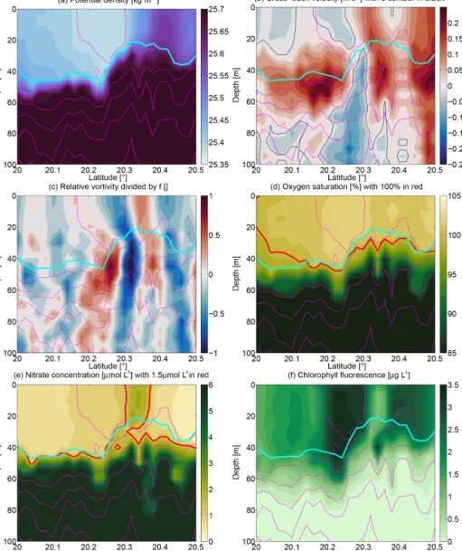
We now investigate in more detail the physical processes that may have contributed to supporting the higher productivity away from the influence of the anticyclone. A spatial and color-scale zoom on the upper water column of 55 km in the south of the section is shown in Fig. 10. Around 20.3^◦N the mixed layer shoaled from 50 to 20 m over a horizontal distance of under 10 km, with isopycnals north of this location steeply dropping. Geostrophy led to the opposing cross-track velocities of ±0.25 m s⁻¹ with the cross-track velocity ex- trema in the stratified water column just below the mixed layer. There the stratification was able to sustain the vertical shear without the system becoming Kelvin–Helmholtz unstable (Richardson number .1/4). The horizontal velocity shear resulted in the large relative vorticity divided by f of up to+1 and below−1 with the region ofζ /f <−1 and consequently negative potential vorticity at 20.32^◦N (Fig. 6d). We hypothesize that this made the region suscep- tible to rapid readjustment via symmetric instability associated with fluid exchange in the vertical and horizontal. Given that PV (a dynamically active parameter; Fig. 6d) was also enhanced at the surface, a simple diffusive process bringing, e.g., nitrate to the surface is not sufficient to explain the observations. Rather the vertical exchange likely also contained an exchange of fluid between the mixed layer and the thermocline below. From the available measurements it is not possible to distinguish whether this mixed layer/base of the mixed layer feature was an eddy, a front, or a filament, but it is clear that very active dynamics were associated with it.

The observation of negative potential vorticity suggests that the situation we observed is likely to have been ongoing for only 1–2 d. That timescale is similar to the phytoplankton doubling time in that part of the ocean, meaning that a large number of doublings and associated POC increase/nutrient drawdown likely did not take place during the time that the situation had been ongoing. The biogeochemical measurements (Fig. 10d–f) corroborate this. In the mixed layer less than a few kilometers north of the region of negative potential vorticity (i.e., north of 20.3^◦N), the nitrate values were enhanced (&2 µmol L⁻¹) with lower (nighttime) chlorophyll-a values than elsewhere in the mixed layer and slightly lower oxygen saturation. This suggests that the nutrient-rich water from below the euphotic zone had been recently injected into

the mixed layer with phytoplankton unable to take the nutrients up in the time available since injection. By contrast, it is likely that the dynamic physical environment had im- pacted the mixed layer both at 5–10 km to the south and to the north in a similar manner (e.g., symmetric instability), several days to a few weeks earlier. We speculate that phytoplankton there grew to large concentrations which increased oxygen and drew down the nitrate. However, the achieved nitrate values are not nearly as close to zero as above the anticyclone where the slower physical evolution of the system over months probably provided phytoplankton of all size classes sufficient time to reduce nitrate to the observed values of as little as 0.01 µmol L⁻¹.

4 Conclusions

In our study, we have shown the structure of anO(100 km) (on the order of 100 km) diameter anticyclonic mode water eddy, anO(20 km) wide mesoscale upwelling filament, and severalO(5–10 km) wide submesoscale mixed layer instabilities in the region offshore of the northwest African upwelling system. We used the physical observations to suggest explanations for the observed differences in the biogeochem- istry and biology along the section both in the mixed layer and below. The single transect without cross-track resolution provides a snapshot of the processes that control the scales of biogeochemical variability in the region, but the lack of cross-track resolution does not allow us to scale this up to quantify the impact of these processes for the region.

The driving mechanism for the mixed layer eddies/filaments in the southern half of the section is not fully clear. The initial creation of negative potential vorticity (PV) is likely to be a key driver. It seems highly probable that once the negative PV was created, symmetric instability would have restored the potential vorticity back to zero. Down-front winds may drive the PV to negative values, but at this point we lack a detailed understanding of the orientation of the fronts with respect to the wind. This would require surveys resolving two horizontal dimensions by a number of parallel sections.

The intricate interplay of different parameters at the kilometer scale needs to be taken into account when interpret- ing single-profile and/or bottle data in such dynamically active regions of the ocean. Additionally, our observations re- inforce the notion that the coupling and decoupling of biological and physical timescales play a key role driving spatial variability. We documented physical forcing ranging in spatial scale from kilometers to hundreds of kilometers, cov- ering timescales ranging from days (for mixed layer instabilities) to months (for ACME advection). These variations then interact with plankton communities at physiological timescales (hours to days) and ecological (weeks) timescales, resulting variously in either an increase (where coupled) or a smoothing (where uncoupled) of the spatial variability. Fi-

(15)

Figure 10.Sections zoomed in on the upper 100 m over 55 km in the south of the transect.(a)Potential density (in kilograms per cubic meter), (b)cross-track velocity (in meters per second),(c)relative vorticity divided byf,(d)oxygen saturation (in percent),(e)nitrate concentration (in micromoles per liter), and(f)chlorophyll-afluorescence (in micrograms per liter).

nally, this study has demonstrated that the TRIAXUS plat- form in its present setup is an ideal tool for interdisciplinary research, especially where interesting physical and biological/biogeochemical dynamics with spatial gradients exist such as eddies, fronts, and filaments.

Data availability. The TRIAXUS, CTD, VMADCP, and thermosalinograph data are available at:

https://doi.org/10.1594/PANGAEA.898716 (Strass, 2019), https://doi.org/10.1594/PANGAEA.895581 (Strass and Rohardt, 2019), https://doi.org/10.1594/PANGAEA.904420 (von Appen et al., 2019), and https://doi.org/10.1594/PANGAEA.897092 (Witte, 2019) (the Pangaea references listed in Sect. 2). The satellite data are available at: http://marine.copernicus.eu (Copernicus, 2020), https://www.esrl.noaa.gov/psd/data/

gridded/data.noaa.oisst.v2.highres.html (NOAA, 2020), and https://esa-oceancolour-cci.org (ESA, 2020) (listed in Sect. 2).

The following data are provided in the Supplement: Supple- ment 1: table_suppl_material.xlsx: nutrient, POC, total and phytoplankton group chlorophyll-a concentration data from underway samples at 11 m and averaged over 0–30 m. Total chlorophyll-ais the sum of the seven phytoplankton groups which can be predicted from the RAMSES sensor data. Supplement 2:

table_suppl_material_WaMoS.xlsx: WaMoS surface current data.

Supplement. SSH_animated.pdf: animation of sea level anomaly and surface geostrophic velocities in the region as in Fig. 2b over the 2.5 months preceding the section presented here. The PDF file needs to be opened with Adobe Reader for animation

(16)

to work. The supplement related to this article is available online at: https://doi.org/10.5194/os-16-253-2020-supplement.

Author contributions. W-JvA conceived the analysis and wrote the paper. VHS conceived the measurements. W-JvA, VHS, AB, HX, and CH collected and analyzed the data. MHI and AMW assisted in the analysis. All authors interpreted the data and commented on the paper.

Competing interests. The authors declare that they have no conflict of interest.

Acknowledgements. We thank Hauke Becker, Susanne Spahic, Jonas Hagemann, and Saad El Naggar for their invaluable help in collecting and processing the data presented here. Support for this study was provided by the Helmholtz Infrastructure Initiative FRAM. We thank Sonja Wiegmann for supporting phytoplankton pigment water sample collection and radiometry data. We thank Sonja Wiegmann and Beke Bracher for HPLC sample analysis.

We acknowledge ACRI-ST for supporting Hongyan Xi’s partic- ipation in PS113 via the project OLCI-PFT. We thank ESA for OC-CCI chlorophyll, Copernicus Marine Environmental Monitor- ing Services (CMEMS) for SLA and NOAA for SST data. Ship time was provided under grant AWI_PS113_00.

Financial support. This research has been supported by the Alfred Wegener Institute, Helmholtz Centre for Polar and Marine Research (grant no. AWI_PS113_00), the Helmholtz Asso- ciation (grant no. FRAM), and the ACRI-ST (grant no. OLCI-PFT).

The article processing charges for this open-access publication were covered by a Research

Centre of the Helmholtz Association.

Review statement. This paper was edited by Piers Chapman and re- viewed by two anonymous referees.

References

Aiken, J., Pradhan, Y., Barlow, R., Lavender, S., Poulton, A., Holligan, P., and Hardman-Mountford, N.: Phytoplankton pigments and functional types in the Atlantic Ocean: a decadal assessment, 1995–2005, Deep-Sea Res. Pt. II, 56, 899–917, https://doi.org/10.1016/j.dsr2.2008.09.017, 2009.

Bachmann, J., Heimbach, T., Hassenrück, C., Kopprio, G. A., Iversen, M. H., Grossart, H. P., and Gärdes, A.: Environmental drivers of free-living vs. particle-attached bacterial community composition in the Mauritania upwelling system, Front. Micro- biol., 9, 1–13, https://doi.org/10.3389/fmicb.2018.02836, 2018.

Barlow, R., Cummings, D., and Gibb, S.: Improved resolution of mono-and divinyl chlorophylls a and b and zeax- anthin and lutein in phytoplankton extracts using reverse

phase C-8 HPLC, Mar. Ecol.-Prog. Ser., 161, 303–307, https://doi.org/10.3354/meps161303, 1997.

Bracher, A., Taylor, M. H., Taylor, B., Dinter, T., Röttgers, R., and Steinmetz, F.: Using empirical orthogonal functions derived from remote-sensing reflectance for the prediction of phytoplankton pigment concentrations, Ocean Sci., 11, 139–158, https://doi.org/10.5194/os-11-139-2015, 2015.

Bracher, A., Xi, H., Dinter, T., Mangin, A., Strass, V., von Appen, W.-J., and Wiegmann, S.: High resolution water column phytoplankton composition across the Atlantic Ocean from ship-towed vertical undulating radiometry, Front. Mar. Sci., in review, 2020.

Capet, X., McWilliams, J. C., Molemaker, M. J., and Shchep- etkin, A.: Mesoscale to submesoscale transition in the Cal- ifornia Current System. Part I: Flow structure, eddy flux, and observational tests, J. Phys. Oceanogr., 38, 29–43, https://doi.org/10.1175/2007JPO3671.1, 2008a.

Capet, X., McWilliams, J. C., Molemaker, M. J., and Shchepetkin, A.: Mesoscale to submesoscale transition in the California Cur- rent System. Part II: Frontal processes, J. Phys. Oceanogr., 38, 44–64, https://doi.org/10.1175/2007JPO3672.1, 2008b.

Chavez, F. P. and Messié, M.: A comparison of eastern boundary upwelling ecosystems, Prog. Oceanogr., 83, 80–96, https://doi.org/10.1016/j.pocean.2009.07.032, 2009.

Chelton, D. B., Deszoeke, R. A., Schlax, M. G., El Nag- gar, K., and Siwertz, N.: Geographical variability of the first baroclinic Rossby radius of deformation, J. Phys.

Oceanogr., 28, 433–460, https://doi.org/10.1175/1520- 0485(1998)028<0433:GVOTFB>2.0.CO;2, 1998.

Cisewski, B. and Strass, V. H.: Acoustic insights into the zooplankton dynamics of the eastern Weddell Sea, Prog. Oceanogr., 144, 62–92, https://doi.org/10.1016/j.pocean.2016.03.005, 2016.

Clark, D. R., Widdicombe, C. E., Rees, A. P., and Woodward, E.

M. S.: The significance of nitrogen regeneration for new production within a filament of the Mauritanian upwelling system, Biogeosciences, 13, 2873–2888, https://doi.org/10.5194/bg-13- 2873-2016, 2016.

Copernicus: Copernicus Marine Environment Monitoring Service, available at: http://marine.copernicus.eu, last access: 25 Febru- ary 2020.

Deines, K. L.: Backscatter estimation using broadband acoustic Doppler current profilers, in: Proceedings of the IEEE Sixth Working Conference on Current Mea- surement (Cat. No. 99CH36331), 249–253, IEEE, https://doi.org/10.1109/CCM.1999.755249, 1999.

d’Ovidio, F., De Monte, S., Della Penna, A., Cotté, C., and Guinet, C.: Ecological implications of eddy retention in the open ocean: a Lagrangian approach, J. Phys. A, 46, 254023, https://doi.org/10.1088/1751-8113/46/25/254023, 2013.

ESA: ESA Climate Change Initiative, Ocean Colour CCI Ver- sion 4.2, available at: https://esa-oceancolour-cci.org, 25 Febru- ary 2020.

Falkowski, P. and Kolber, Z.: Variations in chlorophyll fluorescence yields in phytoplankton in the world oceans, Funct. Plant Biol., 22, 341–355, https://doi.org/10.1071/PP9950341, 1995.

Grasshoff, K., Kremling, K., and Ehrhardt, M.: Methods of seawater analysis, John Wiley & Sons, 2009.

Haine, T. and Marshall, J.: Gravitational, Symmetric, and Baroclinic Instability of the Ocean Mixed Layer, J. Phys.